Robust Control Theory and Applications Part 13 doc

θ
X
1
X
2
(x
1
, x
2
)
v
1
v
2
R
L
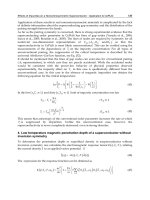
Fig. 3. The one axis car
4.1 Controller design
System (30) is differentially flat, with flat outputs given by the pair of coordinates: (x
1
, x
2
),
which describes the position of the rear axis middle point. Indeed the rest of the system
variables, including the inputs are differentially parameterized as follows:
θ
= arctan

˙
x

2
˙
x
1

, u
1
=

˙
x
2
1
+
˙
x
2
2
, u
2
=
¨
x
2
˙
x
1
−
˙
x

2
¨
x
1
˙
x
2
1
+
˙
x
2
2
Note that the relation between the inputs and the flat outputs highest derivatives is not
invertible due to an ill defined relative degree. To overcome this obstacle to feedback
linearization, we introduce, as an extended auxiliary control input, the time derivative of u
1
.
We have:
˙
u
1
=
˙
x
1
¨
x
1
+

˙
x
2
¨
x
2

˙
x
2
1
+
˙
x
2
2
This control input extension yields now an invertible control input-to-flat outputs highest
derivatives relation, of the form:

˙
u
1
u
2

=
⎡
⎣
˙
x

1
√
˙
x
2
1
+
˙
x
2
2
˙
x
2
√
˙
x
2
1
+
˙
x
2
2
−
˙
x
2
˙
x

2
1
+
˙
x
2
2
˙
x
1
˙
x
2
1
+
˙
x
2
2
⎤
⎦

¨
x
1
¨
x
2

(31)

468
Robust Control, Theory and Applications
4.2 Observer-based GPI controller design
Consider the following multivariable feedback controller based on linear GPI controllers and
estimated cancelation of the nonlinear input matrix gain:

˙
u
1
u
2

=
⎡
⎢
⎢
⎢
⎣
ˆ
˙
x
1

(
ˆ
˙
x
1
)
2

+(
ˆ
˙
x
2
)
2
ˆ
˙
x
2

(
ˆ
˙
x
1
)
2
+(
ˆ
˙
x
2
)
2
−
ˆ
˙
x

2
(
ˆ
˙
x
1
)
2
+(
ˆ
˙
x
2
)
2
ˆ
˙
x
1
(
ˆ
˙
x
1
)
2
+(
ˆ
˙
x

2
)
2
⎤
⎥
⎥
⎥
⎦

ν
1
ν
2

(32)
with the auxiliary control variables, ν
1
, ν
2
,givenby
1
:
ν
1
=
¨
x
∗
1
(t) −


k
12
s
2
+ k
11
s + k
10
s(s + k
13
)

(
x
1
−x
∗
1
(t)
)
ν
2
=
¨
x
∗
2
(t) −


k
22
s
2
+ k
21
s + k
20
s(s + k
23
)

(
x
2
−x
∗
2
(t)
)
(33)
and where the estimated velocity variables:
ˆ
˙
x
1
,
ˆ
˙
x

2
, are generated, respectively, by the variables
ρ
11
and ρ
12
in the following single iterated integral injection GPI observers (i.e., with m = 1),
˙
ˆ
y
10
=
ˆ
y
1
+ λ
13
(y
10
−
ˆ
y
10
)
˙
ˆ
y
1
= ρ
11

+ λ
12
(y
10
−
ˆ
y
10
)
˙
ρ
11
= ρ
21
+ λ
11
(y
10
−
ˆ
y
10
) (34)
˙
ρ
21
= λ
10
(y
10

−
ˆ
y
10
)
y
10
=

t
0
x
1
(τ)dτ
˙
ˆ
y
20
=
ˆ
y
2
+ λ
23
(y
20
−
ˆ
y
20

)
˙
ˆ
y
2
=ρ
12
+ λ
22
(y
20
−
ˆ
y
20
)
˙
ρ
12
=ρ
22
+ λ
21
(y
20
−
ˆ
y
20
) (35)

˙
ρ
22
=λ
20
(y
20
−
ˆ
y
20
)
y
20
=

t
0
x
2
(τ)dτ
Then, the following theorem describes the effect of the proposed integral injection observers,
and of the GPI controllers, on the closed loop system:
Theorem 7. Given a set of desired reference trajectories,
(x
∗
(t), y
∗
(t)), for the desired
position in the plane of the kinematic model of the car, described by (30); given a

set initial conditions,
(x(0), y(0)), sufficiently close to the initial value of the desired
nominal trajectories,
(x
∗
(0), y
∗
(0)), then, the above described GPI observers and the linear
multi-variable dynamical feedback controllers, (32)-(35), forces the closed loop controlled
system trajectories to asymptotically converge towards a small as desired neighborhood of
the desired reference trajectories,
(x
∗
1
(t), x
∗
2
(t)), provided the observer and controller gains
1
Here we have combined, with an abuse of notation, frequency domain and time domain signals.
469
Robust Linear Control of Nonlinear Flat Systems
are chosen so that the roots of the corresponding characteristic polynomials describing,
respectively, the integral injection estimation error dynamics and the closed loop system, are
located deep into the left half of the complex plane. Moreover, the greater the distance of
these assigned poles to the imaginary axis of the complex plane, the smaller the neighborhood
that ultimately bounds the reconstruction errors, the trajectory tracking errors, and their time
derivatives.
Proof. Since the system is differentially flat, in accordance with the results in Maggiore
& Passino (2005), it is valid to make use of the separation principle, which allows us to

propose the above described GPI observers. The characteristic polynomials associated with
the perturbed integral injection error dynamics of the above GPI observers, are given by,
P
ε1
(s)=s
4
+ λ
13
s
3
+ λ
12
s
2
+ λ
11
s + λ
10
P
ε2
(s)=s
4
+ λ
23
s
3
+ λ
22
s
2

+ λ
21
s + λ
20
s ∈ C
thus, the λ
i,j
, i = 1, 2, j = 0, ···, 3, are chosen to identify, term by term, the above estimation
error characteristic polynomials with the following desired stable injection error characteristic
polynomials,
P
ε1
(s)=P
ε2
(s)=(s + 2μ
1
σ
1
s + σ
2
1
)(s + 2μ
2
σ
2
s + σ
2
2
)
s ∈ C, μ

1
, μ
2
, σ
1
, σ
2
∈ R
+
Since the estimated states,
ˆ
˙
x
1
= ρ
11
,
ˆ
˙
x
2
= ρ
12
, asymptotically exponentially converge towards
a small as desired vicinity of the actual states:
˙
x
1
,
˙

x
2
, substituting (32) into (31), transforms
the control problem into one of controlling two decoupled double chains of integrators. One
obtains the following dominant linear dynamics for the closed loop tracking errors:
e
(4)
1
+ k
13
e
(3)
1
+ k
12
¨
e
1
+ k
11
˙
e
1
+ k
10
e
1
= 0 (36)
e
(4)

2
+ k
23
e
(2)
2
+ k
22
¨
e
2
+ k
21
˙
e
2
+ k
20
e
2
= 0 (37)
The pole placement for such dynamics has to be such that both corresponding associated
characteristic equations guarantee a dominant exponentially asymptotic convergence. Setting
the roots of these characteristic polynomials to lie deep into the left half of the complex plane
one guarantees an asymptotic convergence of the perturbed dynamics to a small as desired
vicinity of the origin of the tracking error phase space.
4.3 Experimental results
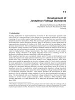
An experimental implementation of the proposed controller design method was carried out
to illustrate the performance of the proposed linear control approach. The used experimental
prototype was a parallax “Boe-Bot" mobile robot (see figure 5). The robot parameters are the

following: The wheels radius is R
= 0.7 [m]; its axis length is L = 0.125 [m]. Each wheel
radius includes a rubber band to reduce slippage. The motion system is constituted by two
servo motors supplied with 6 V dc current. The position acquisition system is achieved by
means of a color web cam whose resolution is 352
× 288 pixels. The image processing was
carried out by the MATLAB image acquisition toolbox and the control signal was sent to the
robot micro-controller by means of a wireless communication scheme. The main function of
470
Robust Control, Theory and Applications
the robot micro-controller was to modulate the control signals into a PWM input for the motor.
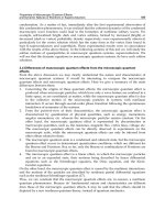
The used micro-controller was a BASIC Stamp 2 with a blue-tooth communication card. Figure
4 shows a block diagram of the experimental framework. The proposed tracking tasks was a
six-leaved “rose" defined as follows:
x
∗
1
(t)=sin(3ωt + η) sin(2ωt + η)
x
∗
2
(t)=sin(3ωt + η) cos(2ωt + η)
The design parameters for the observers were set to be, μ
1
= 1.8, μ
2
= 2.3, σ
1
= 3, σ
2

= 4
and for the corresponding parameters for the controllers, ζ
1
= ζ
3
= 1.2, ζ
2
= ζ
4
= 1.5,
ω
n1
= ω
n3
= 1.8, ω
n2
= ω
n4
= 1.9. Also, we compared the observer response with that
of a GPI observer without the integral injection
(x
1_
, x
2_
) Luviano-Juárez et al. (2010). The
experimental implementation results of the control law are depicted in figures, 6 and 7, where
the control inputs and the tracking task are depicted. Notice that in the case of figure 8, there is
a clear difference between the integral injection observer and the usual observer; the filtering
effect of the integral observer helped to reduce the high noisy fluctuations of the control input
due to measurement noises. On the average, the absolute error for the tracking task, for booth

schemes, is less than 1 [cm]. This is quite a reasonable performance considering the height of
the camera location and its relatively low resolution.
DC Motor 1 DC Motor 2
Micro
Controller
Bluetooth
Antenna
USB Camera
USB
Port
Target
PC
Bluetooth
Transmitter
PWM
1
PWM
2
Nonholonomic Car
Fig. 4. Experimental control schematics
471
Robust Linear Control of Nonlinear Flat Systems
Fig. 5. Mobile Robot Prototype
5. Conclusions
In this chapter, we have proposed a linear observer-linear controller approach for the robust
trajectory tracking task in nonlinear differentially flat systems. The nonlinear inputs-to-flat
outputs representation is viewed as a linear perturbed system in which only the orders of
integration of the Kronecker subsystems and the control input gain matrix of the system are
considered to be crucially relevant for the controller design. The additive nonlinear terms
in the input output dynamics can be effectively estimated, in an approximate manner, by

means of a linear, high gain, Luenberger observer including finite degree, self updating,
polynomial models of the additive state dependent perturbation vector components. This
perturbation may also include additional unknown external perturbation inputs of uniformly
absolutely bounded nature. A close approximate estimate of the additive nonlinearities is
guaranteed to be produced by the linear observers thanks to customary, high gain, pole
placement procedure. With this information, the controller simply cancels the disturbance
vector and regulates the resulting set of decoupled chain of perturbed integrators after a
direct nonlinear input gain matrix cancelation. A convincing simulation example has been
presented dealing with a rather complex nonlinear physical system. We have also shown
that the method efficiently results in a rather accurate trajectory tracking output feedback
controller in a real laboratory implementation. A successful experimental illustration was
presented which considered a non-holonomic mobile robotic system prototype, controlled by
an overhead camera.
472
Robust Control, Theory and Applications
0 50 100 150 200
0
0.1
0.2
Time [s]
u
1
[m/s]
0 50 100 150 200
−2
0
2
Time [s]
u
2

[m/s]
Fig. 6. Experimental applied control inputs
−0.6 −0.4 −0.2 0 0.2 0.4 0.6
−0.6
−0.4
−0.2
0
0.2
0.4
0.6
x
1
[m]
x
2
[m]


Reference Tracking
Fig. 7. Experimental performance of GPI observer-based control on trajectory tracking task
473
Robust Linear Control of Nonlinear Flat Systems
0 50 100 150 200
−0.1
−0.05
0
0.05
0.1
Time [s]

˙
ˆx
1
˙
ˆx
1
˙x
1
0 50 100 150 200
−0.1
−0.05
0
0.05
0.1
Time [s]


˙
ˆx
2
˙
ˆx
2
˙x
2
Fig. 8. Noise reduction effect on state estimations via integral error injection GPI observers
6.References
Aguilar, L. E., Hamel, T. & Soueres, P. (1997). Robust path following control for wheeled robots
via sliding mode techniques, International Conference of Intelligent Robotic Systems,

pp. 1389–1395.
Bazanella, A. S., Kokotovic, P. & Silva, A. (1999). A dynamic extension for l
g
v controllers, IEEE
Transactions on Automatic Control 44(3).
Cortés-Romero, J., Luviano-Juárez, A. & Sira-Ramírez, H. (2009). Robust gpi controller for
trajectory tracking for induction motors, IEEE International Conference on Mechatronics,
Málaga, Spain, pp. 1–6.
Diop, S. & Fliess, M. (1991). Nonlinear observability, identifiability and persistent trajectories,
Proceedings of the 36th IEEE Conference on Decision and Control, Brighton, England,
pp. 714 – 719.
Dixon, W., Dawson, D., Zergeroglu, E. & Behal, A. (2001). Nonlinear Control of Wheeled Mobile
Robots, Vol. 262 of Lecture Notes in Control and Information Sciences,Springer,Great
Britain.
Fliess, M. & Join, C. (2008). Intelligent PID controllers, Control and Automation, 2008 16th
Mediterranean Conference on, pp. 326 –331.
Fliess, M., Join, C. & Sira-Ramirez, H. (2008). Non-linear estimation is easy, International Journal
of Modelling, Identification and Control 4(1): 12–27.
474
Robust Control, Theory and Applications
Fliess, M., Lévine, J., Martin, P. & Rouchon, P. (1995). Flatness and defect of non-linear systems:
introductory theory and applications, International Journal of Control 61: 1327–1361.
Fliess, M., Marquez, R., Delaleau, E. & Sira-Ramírez, H. (2002). Correcteurs proportionnels
intègraux généralisés, ESAIM: Control, Optimisation and Calculus of Variations
7(2): 23–41.
Fliess, M. & Rudolph, J. (1997). Corps de hardy et observateurs asymptotiques locaux pour
systèmes différentiellement plats, C.R. Academie des S ciences de Paris 324, Serie II
b: 513–519.
Gao, Z. (2006). Active disturbance rejection control: A paradigm shift in feedback
control system design, American Control Conference, Minneapolis, Minnesota, USA,

p. 2399
˝
U2405.
Gao, Z., Huang, Y. & Han, J. (2001). An alternative paradigm for control system design, 40th
IEEE Conference on Decision and Control, Vol. 5, pp. 4578–4585.
Han, J. (2009). From PID to active disturbance rejection control, IEEE Transactions on Industrial
Electronics 56(3): 900–906.
Hingorani, N. G. & Gyugyi, L. (2000). Understanding FACTS, IEEE Press, Piscataway, N.J.
Hou, Z., Zou, A., Cheng, L. & Tan, M. (2009). Adaptive control of an electrically driven
nonholonomic mobile robot via backstepping and fuzzy approach, IEEE Transactions
on Control Systems Technology 17(4): 803–815.
Johnson, C. D. (1971). Accommodation of external disturbances in linear regulator and
servomechanism problems, IEEE Transactions on Automatic Control AC-16(6).
Johnson, C. D. (1982). Control and Dynamic Systems: Advances in Theory and applications, Vol. 18,
Academic Press, NY, chapter Discrete-Time Disturbance-Accommodating Control
Theory, pp. 224–315.
Johnson, C. D. (2008). Real-time disturbance-observers; origin and evolution of the idea. part
1: The early years, 40th Southeastern Symposium on System Theory,NewOrleans,LA,
USA.
Kailath, T. (1979). Linear Systems, Information and System Science Series, Prentice-Hall, Upper
Saddle River, N.J.
Kim, D. & Oh, J. (1999). Tracking control of a two-wheeled mobile robot using input-output
linearization, Control Engineering Practice 7(3): 369–373.
Leroquais, W. & d’Andrea Novel, B. (1999). Modelling and control of wheeled mobile robots
not satisfying ideal velocity constraints: The unicycle case, European Journal of Control
5(2-4): 312–315.
Luenberger, D. (1971). An introduction to observers, IEEE Transactions on Automatic Control
16: 592–602.
Luviano-Juárez, A., Cortés-Romero, J. & Sira-Ramírez, H. (2010). Synchronization of chaotic
oscillators by means of generalized proportional integral observers, International

Journal of Bifurcation and Chaos 20(5): 1509
˝
U–1517.
Maggiore, M. & Passino, K. (2005). Output feedback tracking: A separation principle
approach, IEEE Transactions on Automatic Control 50(1): 111–117.
Mohadjer, M. & Johnson, C. D. (1983). Power system control with
disturbance-accommodation, 22nd IEEE Confer e nce on Conference on Decision and
Control, San Antonio, Texas.
Pai, M. A. (1989). Energy Function Analysis for Power System Stability,KluwerAcademic
Publishers.
475
Robust Linear Control of Nonlinear Flat Systems
Parker, G. A. & Johnson, C. D. (2009). Decoupling linear dynamical systems using
disturbance accommodation control theory, 41st Southeastern Symposium on System
Theory,Tullahoma,TN,USA.
Peng, J., Wang, Y. & Yu, H. (2007). Advances in Neural Networks, Vol. 4491 of Lecture Notes
in Computer Science, Springer Berlin / Heidelberg, chapter Neural Network-Based
Robust Tracking Control for Nonholonomic Mobile Robot, pp. 804–812.
Pomet, J. (1992). Explicit design of time-varying stabilizing control laws for a class of
controllable systems without drift., Systems and Control Letters 1992 18(2): 147–158.
Samson, C. (1991). Advanced Robot Control, Vol. 162 of Lecture Notes in Control and Information
Sciences, Springer, chapter Velocity and torque feedback control of a nonholonomic
cart, pp. 125–151.
Sira-Ramírez, H. & Agrawal, S. (2004). Differentially flat systems, Marcel Dekker Inc.
Sira-Ramírez, H. & Feliu-Battle, V. (2010). Robust σ
− δ modulation based sliding mode
observers for linear systems subject to time polynomial inputs, International Journal of
Systems Science . To appear.
Sira-Ramírez, H. & Fliess, M. (2004). On the output feedback control of a synchronous
generator, Proceedings of the 43rd. IEEE Conference on Decision and Control, Bahamas.

Sugisaka, M. & Hazry, D. (2007). Development of a proportional control method for a mobile
robot, Applied Mathematics and Computation 186: 74–82.
Sun, B. & Gao, Z. (2005). A dsp-based active disturbance rejection control design for a
1-kw h-bridge dc
˝
Udc power converter, IEEE Transactions on Industrial Electronics
52(5): 1271
˝
U1277.
Sun, D. (2007). Comments on active disturbance rejection control, IEEE Transactions on
Industrial Electronics 54(6): 3428–3429.
Tian, Y. & Cao, K. (2007). Time-varying linear controllers for exponential tracking of
non-holonomic systems in chained form, International Journal of Robust and Nonlinear
Control 17: 631–647.
Wang, Z., Li, S. & Fei, S. (2009). Finite-time tracking control of a nonholonomic mobile robot,
Asian Journal of Control 11(3): 344–357.
Wit, C. C. D. & Sordalen, O. (1992). Exponential stabilization of mobile robots with
nonholonomic constraints, IEEE Transactions on Automatic Control 37(11): 1791–1797.
Yang, J. & Kim, J. (1999). Sliding mode control for trajectory tracking of nonholonomic
wheeled mobile robots, IEEE Transactions on Robotics and Automation 15(3): 578–587.
476
Robust Control, Theory and Applications
Part 5
Robust Control Applications

Hao Zhang
1
and Huaicheng Yan
2
1

Department of Control Science and Engineering, Tongji University, Shanghai 200092
2
School of Information Science and Engineering, East China University of Science and
Technology,Shanghai 200237
PRChina
1. Introduction
The Internet is playing an important role in information retrieval, exchange, and applications.
Internet-based control, a new type of control systems, is characterized as globally remote
monitoring and adjustment of plants over the Internet. In recent years, Internet-based
control systems have gained considerable attention in science and engineering [1-6], since
they p rovide a new and convenient unified f ramework for system control and practical
applications. Examples include intelligent home environments, windmill and solar power
stations, small-scale hydroelectric power stations, and other highly geographically distributed
devices, as well as tele-manufacturing, tele-surgery, and tele-control of spacecrafts.
Internet-based control is an interesting and challenging topic. One of the major challenges
in Internet-based control systems is how to deal with the Internet transmission delay. The
existing approaches of overcoming network transmission delay mainly focus on designing
a model based time-delay compensator or a state observer to reduce the effect of the
transmission delay. Being distinct from the existing approaches, literatures (7–9) have been
investigating the overcoming of the Internet time-delay from the control system architecture
angle, including introducing a tolerant time to the fixed sampling interval to potentially
maximize the possibility of succeeding the transmission on time. Most recently, a dual-rate
control scheme for Internet-based control systems has been proposed in literature (10). A
two-level hierarchy was used in the dual-rate control scheme. At the lower level a local
controller which is implemented to control the plant at a higher frequency to stabilize the
plant and guarantee the plant being under control even the network communication is lost
for a long time. At the higher level a remote controller is employed to remotely regulate the
desirable reference at a lower frequency to reduce the communication load and increase the
possibility of receiving data over the Internet on time. The local and the remote controller are
composed of some modes, which mode is enabled due to the time and state of the network.

The mode may changes at instant time k, k
∈{N
+
} and at each instant time only one mode
of the controller is enabled. A typical dual-rate control scheme is demonstrated in a process
control rig (7; 8) and has shown a great potential to over Internet time-delay and bring this
new generation of control systems into industries. However, since the time-delay is variable
and the uncertainty of the process parameters is unavoidable, a dual-rate Internet-based
control system may be unstable for certain control intervals. The interest in the stability of
Passive Robust Control for Internet-Based
Time-Delay Switching Systems

21
networked control systems have grown in recent years due to its theoretical and practical
significance [11-21], but to our knowledge there are very few reports dealing with the robust
passive control for such kind of Internet-based control systems. The robust passive control
problem for time-delay systems was dealt with in (24; 25). This motivates the present passivity
investigation of multi-rate Internet-based switching control systems with time-delay and
uncertainties.
In this paper, we study the modelling and robust passive control for Internet-based switching
control systems with multi-rate scheme, time-delay, and uncertainties. The controller is
switching between some modes due to the time and state of the network, either different time
or the state changing may cause the controller changes its mode and the mode may changes at
each instant time. Based on remote control and local control strategy, a new class of multi-rate
switching control model with time-delay is formulated. Some new robust passive properties
of such systems under arbitrary switching are investigated. An example is given to illustrate
the effectiveness of the theoretical results.
Notation: Through the paper I denotes identity matrix of appropriate order, and
∗ represents
the elements below the main diagonal o f a symmetric block m atrix. The superscript


represents the transpose. L
2
[0, ∞) refers to the space of square summable infinite vector
sequences. The notation X
> 0(≥ , <, ≤ 0) denotes a symmetric positive definite (positive
semi-definite, negative, negative semi-definite) matrix X. Matrices, if not explicitly stated, are
assumed to have compatible dimensions. Let N
= {1, 2, ···}and N
+
= {0, 1,2, ···}denote
the sets of positive integer and nonnegative integer, respectively.
2. Problem formulation
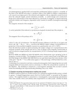
A typical multi-rate control structure with remote controller and local controller can be shown
as Fig. 1. The control architrave gives a discrete dynamical system, where plant is in circle
with broken line, x
(k) ∈ R
n
is the system state, z(k) ∈ R
q
is the output, and ω(k) ∈ R
p
is
the exogenous input, which is assumed to belong to L
2
[0, ∞), r(k) is the input and for the
passivity analysis one can let r
(k)=0, u
1
(k) and u

2
(k) are the output of remote control
and local control, respectively. A
1
, B
1
, B
2
and C are parameter matrices of the model with
appropriate dimensions, K
2i
and K
1j
are control gain switching matrices where the switching
rules are given by i
(k)=s(x(k), k) and j(k)=σ(x (k), k),andi ∈{1, 2, ···, N
1
}, j ∈
{
1, 2, ···, N
2
}, N
1
, N
2
∈ N, which imply that the switching controllers have N
1
and N
2
modes,

respectively. τ
1
and τ
2
are time-delays caused by communication delay in systems.
For the system given by Fig. 1, it is assumed that, the sampling interval of remote controller is
the m multiple of local controller with m being positive integer, and the switching device
SW1 closes only at the instant time k
= nm, n ∈ N
+
, and otherwise, it switches off.
Correspondingly, remote controller u
1
(k) updates its state at k = nm, n ∈ N
+
only, and
otherwise, it keeps invariable. Also, it is assumed t hat the benchmark of discrete systems is
the same as local controller. In this case, the system can be described by the following discrete
system with time-delay
⎧
⎪
⎪
⎨
⎪
⎪
⎩
x
(k + 1)=A
1
x(k)+B

2
u
2
(k)+Eω(k),
u
2
(k)=B
1
u
1
(k − τ
2
) − K
2i
x(k),
z
(k)=Cx(k)+Dω(k ),
(1)
480
Robust Control, Theory and Applications
Fig. 1. Multi-rate network control loop with time-delays
where remote controller u
1
(k − τ
2
) is given by

u
1
(k − τ

2
)= r(k −τ
2
) − K
1j
x(k − τ
1
−τ
2
), k = nm,
u
1
(k − τ
2
)= r(nm −τ
2
) − K
1j
x(nm − τ
1
−τ
2
), k ∈{nm + 1, ···, nm + m −1},
(2)
with i
∈{1, 2, ···, N
1
}, j ∈{1, 2, ···, N
2
}, k, n ∈ N

+
and N
1
, N
2
∈ N. Moreover, it follows
from (1) and (2) that, for k
= nm,

x
(k + 1)= ( A
1
−B
2
K
2i
) x(k ) − B
2
B
1
K
1j
x(k − τ
1
−τ
2
)+B
2
B
1

r(k − τ
2
)+Eω(k),
z
(k)=Cx(k)+Dω(k ),
(3)
and for k
∈{nm + 1, ···, nm + m −1},

x
(k + 1)= ( A
1
− B
2
K
2i
) x(k ) − B
2
B
1
K
1j
x(nm − τ
1
−τ
2
)+B
2
B
1

r(nm − τ
2
)+Eω(k),
z
(k)=Cx(k)+Dω(k).
(4)
For the passivity analysis, one can let r
(k)=0, and then the system (3) and (4) become
⎧
⎪
⎨
⎪
⎩
x
(k + 1)= ( A
1
− B
2
K
2i
) x(k) − B
2
B
1
K
1j
x(k − τ)+Eω(k), k = nm,
x
(k + 1)= ( A
1

− B
2
K
2i
) x(k) − B
2
B
1
K
1j
x(nm − τ)+Eω(k), k ∈{nm + 1, ···, nm + m −1},
z
(k)=Cx(k)+Dω(k ),
(5)
where τ
= τ
1
+ τ
2
> 0, k ∈ N
+
, n ∈ N
+
, m > 0 is a positive integer.
Obviously, if define A
i
= A
1
− B
2

K
2i
, B
j
= −B
2
B
1
K
1j
, then the controlled system (5) becomes
⎧
⎨
⎩
x
(k + 1)=A
i
x(k)+B
j
x(k − τ)+E ω(k), k = nm,
x
(k + 1)=A
i
x(t)+B
j
x(nm − τ)+Eω(k), k ∈{nm + 1, ···, nm + m −1},
z
(k)=Cx(k)+Dω(k ),
(6)
481

Passive Robust Control for Internet-Based Time-Delay Switching Systems
where A
1
, B
1
, B
2
, C, D, E are matrices with appropriate dimensions, K
1j
and K
2i
aremodegain
matrices of the remote controller and local controller. At each instant time k, there is only
one mode of each controller is enabled. τ
= τ
1
+ τ
2
> 0andm > 0areintegers,k ∈ N
+
,
n
= 0, 1, 2, ···.
Furthermore, note that, as k
= nm + s with s = 0, 1, ··· , m −1, and nm −τ = k −(τ + s) then
(6) can be rewritten as

x
(k + 1)=A
i

x(k)+B
j
x(k − h)+Eω(k),
z
(k)=Cx(k)+Dω(k),
(7)
with 0
≤ τ ≤ h ≤ τ + m −1. Accordingly, for the case of time-varying structured uncertainties
(7) becomes

x
(k + 1)= ( A
i
+ ΔA(k )) x(k)+(B
j
+ ΔB(k)) x(k − h)+(E + ΔE)ω(k),
z
(k)=Cx(k)+Dω(k),
(8)
with 0
≤ τ ≤ h ≤ τ + m − 1, and ΔA(k), ΔB(k) and ΔE being structured uncertainties, and
are assumed to have the form of
ΔA
(k)=D
1
F(k)E
a
, ΔB(k)=D
1
F(k)E

b
, ΔE(k)=D
1
F(k)E
e
,(9)
where D
1
, E
a
, E
b
and E
e
are known constant real matrices with appropriate dimensions. It is
assumed that
F

(k)F(k ) ≤ I, ∀k. (10)
In what follows, the the passive control for the hybrid model (7) and (8) are first studied, and
then, an example of systems (8) is investigated.
3. Passivity analysis
On the basis of models (7) and (8), consider the following discrete-time nominal switching
system with time-delay:
⎧
⎪
⎪
⎪
⎪
⎨

⎪
⎪
⎪
⎪
⎩
x
(k + 1)=A
i
x(k)+B
j
x(k − h)+Eω(k) ,
z
(k)=Cx(k)+Dω(k),
x
(k)=φ(k), k ∈ [−h,0],
i
(k)=s(x(k), k),
j
(k)=σ(x(k), k),
(11)
where s and σ are switching rules, i
∈{1,···, N
1
}, j ∈{1, ···, N
2
}, N
1
, N
2
∈ N, A

i
, B
j
∈ R
n×n
are ith and jth switching matrices of system (11), h ∈ N is the time delay, and φ(·) is the initial
condition.
For the case of structured uncertainties, it can be described by
⎧
⎪
⎪
⎪
⎪
⎨
⎪
⎪
⎪
⎪
⎩
x
(k + 1)=A
i
(k)x(k)+B
j
(k)x(k − h)+E(k)ω(k) ,
z
(k)=Cx(k)+Dω(k),
x
(k)=φ(k ), k ∈ [−h,0],
i

(k)=s(x(k), k),
j
(k)=σ(x(k), k),
(12)
482
Robust Control, Theory and Applications
where A
i
(k)=A
i
+ ΔA(k) , B
j
(k)=B
j
+ ΔB(k) , E(k)=E + ΔE(k), and it is assumed that
(9) and (10) are satisfied. Our problem is to test whether system (11) and (12) are passive with
the switching controllers. To this end, we introduce the following fact and related definition
of passivity.
Lemma 1 (22). The following inequality holds for any a
∈ R
n
a
, b ∈ R
n
b
, N ∈ R
n
a
×n
b

, X ∈
R
n
a
×n
a
, Y ∈ R
n
a
×n
b
,andZ ∈ R
n
b
×n
b
:
−2a

Nb ≤

a
b



XY
− N
∗ Z


a
b

, (13)
where

XY
∗ Z

≥ 0.
Lemma 2 (23). Given matrices Q
= Q

, H, E and R = R

> 0 of appropriate dimensions,
Q
+ HFE+ E

F

H

< 0 (14)
holds for all F satisfying F

F ≤ R, if and only if there exists some λ > 0suchthat
Q
+ λHH


+ λ
−1
E

RE < 0. (15)
Definition 1 (26) The dynamical system (11) is called passive if there exists a scalar β such that
k
f
∑
k=0
ω

(k)z(k) ≥ β, ∀ω ∈ L
2
[0, ∞), ∀k
f
∈ N,
where β is some constant which depends on the initial condition of system.
In the sequel, we provide condition under which a class of discrete-time switching dynamical
systems with time-delay and uncertainties can be guaranteed to be passive.
System (11) can be recast as
⎧
⎪
⎪
⎪
⎪
⎪
⎪
⎪
⎪

⎨
⎪
⎪
⎪
⎪
⎪
⎪
⎪
⎪
⎩
y
(k)= x(k + 1) − x(k),
0
=(A
i
+ B
j
−I)x(k) −y(k)−B
j
k
−1
∑
l=k−h
y(l)+Eω(k),
z
(k)= Cx(k)+Dω(k ),
x
(k)= φ(k), k ∈ [−h,0]
i(k)=s(x(k), k),
j

(k)=σ(x(k), k).
(16)
It is noted that (11) is completely equivalent to (16).
Theorem 1. System (11) is passive under arbitrary switching rules s and σ,ifthereexist
matrices P
1
> 0, P
2
, P
3
, W
1
, W
2
, W
3
, M
1
, M
2
, S
1
> 0, S
2
> 0 such that the following LMIs hold
Λ
=
⎡
⎢
⎢

⎣
Q
1
Q
2
P

2
B
j
− M
1
P

2
E − C
∗ Q
3
P

3
B
j
− M
2
P

3
E
∗∗ −S

2
0
∗∗ ∗ −(D + D

)
⎤
⎥
⎥
⎦
< 0, (17)
and

WM
M

S
1

≥ 0, (18)
483
Passive Robust Control for Internet-Based Time-Delay Switching Systems
for i ∈{1,···, N
1
}, j ∈{1, ···, N
2
}, N
1
, N
2
∈ N,where

Q
1
= P

2
(A
i
− I)+(A
i
− I)

P
2
+ hW
1
+ M
1
+ M

1
+ S
2
,
Q
2
=(A
i
− I)

P

3
+ P

1
− P

2
+ hW
2
+ M

2
,
Q
3
= −P
3
− P

3
+ hW
3
+ P
1
+ hS
1
,
W
=


W
1
W
2
∗ W
3

, M
=

M
1
M
2

.
Proof. Construct Lyapunov function as
V
(k)= x

(k)P
1
x(k)+
0
∑
θ=−h+1
k
−1
∑
l=k−1+θ

y

(l)S
1
y(l)+
k−1
∑
l=k−h
x

(l)S
2
x(l),
then
ΔV(k)= V(k + 1) −V(k)
=
2x

(k)P
1
y(k)+x

(k)S
2
x(k)+y

(k)(P
1
+ hS
1

)y(k)
−
x

(k − h)S
2
x(k − h) −
k−1
∑
l=k−h
y

(l)S
1
y(l),
(19)
where
2x

(k)P
1
y(k)= 2η

(k)P

{

y
(k)
(

A
i
+ B
j
− I)x(k) − y(k)+Eω(k)

−
k−1
∑
l=k−h

0
B
j

y
(l)},
(20)
with η

(k)=

x

(k) y

(k)

, P
=


P
1
0
P
2
P
3

,and
2η

(k)P


y
(k)
(
A
i
+ B
j
− I)x(k) − y(k)+Eω(k)

= 2η

(k)P

{


0
A
i
− I

x
(k)+

I
−I

y
(k)+

0
B
j

x
(k)+

0
Eω
(k)

}.
(21)
According to Lemma 1 we get that
−2
k−1

∑
l=k−h
η

(k)P


0
B
j

y
(l)
≤
k−1
∑
l=k−h

η
(k)
y(l)


⎡
⎣
WM
− P


0

B
j

∗ S
1
⎤
⎦

η
(k)
y(l)

=η

(k)hWη(k)+2η

(k)( M −P


0
B
j

)(x(k) −x(k − h)) +
k−1
∑
l=k−h
y

(l)S

1
y(l),
(22)
where

WM
∗ S
1

≥ 0.
484
Robust Control, Theory and Applications
From (19)-(22) we can get
ΔV
(k) −2z

(k)ω(k)= 2η

(k)P


0 I
A
i
− I −I

η
(k)+η

(k)hWη(k)

+
2η

(k)Mx(k)+2η

(k)(P


0
B
j

− M)x(k −h)+x

(k)S
2
x(k)
+
y

(k)(P
1
+ hS
1
)y(k) −x

(k − h)S
2
x(k − h)+2η


(k)P


0
Eω
(k)

−2(x

(k)C

ω(k)+ω

(k)D

ω(k)).
Let ξ

(k)=[x

(k), y

(k), x

(k −h), ω

(k)],thenΔV(k) −2z

(k)ω(k) ≤ ξ(k)


υξ (k),where
υ =
⎡
⎢
⎢
⎣
φ P


0
B
j

− M

P

2
E − C

P

3
E

∗−S
2
0
∗∗ −(D + D


)
⎤
⎥
⎥
⎦
, (23)
and
φ
=P


0 I
A
i
− I −I

+

0 I
A
i
− I −I


P + hW +

M 0

+


M

0

+

S
2
0
0 P
1
+ hS
1

.
If v
< 0, then V(k) −2z

(k)ω(k) < 0, which gives
k
f
∑
k=0
ω

(k)z(k) >
1
2
k
f

∑
k=0
V(k)=
1
2
[V(k
f
+ 1) − V(0)].
Furthermore, since V
(k)=V(x(k)) ≥ 0, it follows that
k
f
∑
k=0
ω

(k)z(k) ≥−
1
2
V
(0) ≡ β, ∀ω ∈ L
2
[0, ∞), ∀ k
f
∈ N,
which implies from Definition 1 that the system (11) is passive. Using the Schur complement
(23) is equivalent to (17). This complete the proof.
Theorem 2. System (12) is passive under arbitrary switching rules s and σ,ifthere
exist matrices P
1

> 0, P
2
, P
3
, W
1
, W
2
, W
3
, M
1
, M
2
, S
1
> 0, S
2
> 0 such that the following LMIs
holds
⎡
⎢
⎢
⎢
⎢
⎣
Q
1
+E


a
E
a
Q
2
P

2
B
j
−M
1
+E

a
E
b
P

2
E − C

+ E

a
E
e
P

2

D
1
∗ Q
3
P

3
B
j
− M
2
P

3
EP

3
D
1
∗∗−S
2
+ E

b
E
b
E

b
E

e
0
∗∗ ∗ −(D + D

)+E

e
E
e
0
∗∗ ∗ ∗ −I
⎤
⎥
⎥
⎥
⎥
⎦
<0, (24)
and

WM
M

S
1

≥ 0, (25)
for
i
∈{1,···, N

1
}, j ∈{1,··· , N
2
}, N
1
, N
2
∈ N,
485
Passive Robust Control for Internet-Based Time-Delay Switching Systems
where Q
1
, Q
2
, Q
3
, W, M are defined in Theorem 1 and E
a
, E
b
, E
e
are given by (9) and (10).
Proof. Replacing A
i
, B
j
and E in (17) with A
i
+ D

1
F(k)E
a
, B
j
+ D
1
F(k)E
b
and E + D
1
F(k)E
e
,
respectively, we find that (17) for (12) is equivalent to the following condition
Λ
+
⎡
⎢
⎢
⎣
P

2
D
1
P

3
D

1
0
0
⎤
⎥
⎥
⎦
F
(k)

E
a
0 E
b
E
e

+
⎡
⎢
⎢
⎣
E

a
0
E

b
E


e
⎤
⎥
⎥
⎦
F

(k)

D

1
P
2
D

1
P
3
00

< 0.
By Lemma 2, a sufficient condition guaranteeing (17) for (12) is that there exists a positive
number λ
> 0suchthat
λΛ
+ λ
2
⎡

⎢
⎢
⎣
P

2
D
1
P

3
D
1
0
0
⎤
⎥
⎥
⎦

D

1
P
2
D

1
P
3

00

+
⎡
⎢
⎢
⎣
E

a
0
E

b
E

e
⎤
⎥
⎥
⎦

E
a
0 E
b
E
e

< 0. (26)

Replacing λP, λS
1
, λS
2
, λM and λW with P, S
1
, S
2
, M and W respectively, and applying the
Schur complement shows that (26) is equivalent to (24). This completes the proof.
4. A numerical example
In this section, we shall present an example to demonstrate the effectiveness and applicability
of the proposed method. Consider system (12) with parameters as follows:
A
1
=

−6 −6
2
−2

, A
2
=

−4 −6
4
−4

, B

1
=

−1 −2
0
−1

, B
2
=

−20
−3 −1

,
B
3
=

−10
0
−1

C
=

0.1
−0.2

, E =


0.2
0.1

, E
a
=

0.5 0
0.1 0.2

, E
b
=

0.6 0
00.3

, D
1
=

0.1 0
01

,
D
= 0.1, h = 5.
Applying Theorem 2, with i
∈{1,2}, j ∈{1,2, 3}. It has been found by using software LMIlab

that the switching discrete time-delay system (12) is the passive and we obtain the solution as
follows:
P
1
= 10
−3
×

0.1586 0.0154
∗ 0.2660

, P
2
=

0.5577 0.3725
−1.6808 1.0583

, P
3
=

0.1689
−0.0786
−0.0281 0.1000

,
S
1
= 10

−4
×

0.4207 0.0405
∗ 0.6941

, S
2
=

2.6250 0.8397
∗ 2.0706

, W
1
=

0.2173
−0.0929
∗ 0.0988

,
W
2
=

0.0402
−0.0173
∗ 0.0182


, W
3
=

0.0075
−0.0032
∗ 0.0034

, M
1
= 10
−4
×

−0.0640 −0.2109
0.1402
−0.5777

,
M
2
= 10
−5
×

0.0985
−0.4304
0.1231
−0.9483


.
486
Robust Control, Theory and Applications
5. Conclusions
In this paper, based on remote control and local control strategy, a class of hybrid multi-rate
control models with uncertainties and switching controllers have been formulated and their
passive control problems have been investigated. Using the Lyapunov-Krasovskii function
approach on an equivalent singular system, some new conditions in form of LMIs have been
derived. A numerical example has been shown to verify the effectiveness of the proposed
control and passivity methods.
6. Acknowledgements
This work is supported by the Program of the International Science and Technology
Cooperation (No.2007DFA10600), the National Natural Science Foundation of China
(No.60904015, 61004028), the Chen Guang project supported by Shanghai Municipal
Education Commission, Shanghai Education Development Foundation (No.09CG17), the
National High Technology Research and Development Program of China (No.2009AA043001),
the Shanghai Pujiang Program (No.10PJ1402800), the Fundamental Research Funds for the
Central Universities (No.WH1014013) and the Foundation of East China University of Science
and Technology (No.YH0142137).
7.References
[1] Huang J, Guan Z H, Wang Z. Stability of networked control s ystems based on model
of discrete-time interval system with uncertain delay. Dynamics of Continuous, Discrete
and Impulsive Systems Series B: Applications & Algorithms 2004; 11: 35-44.
[2] Lien C H. Further results on delay-dependent robust stability of uncertain fuzzy systems
with time-varying delay. Chaos, Solitons & Fractals 2006; 28(2): 422-427.
[3] Montestruque L A, Antsaklis P J. On the model-based control of networked systems.
Automatica 2003; 39: 1837-43.
[4] Montestruque L A , Antsaklis P J.Stability of model-based networked control systems
with time-varying transmission times. IEEE Trans. Autom. Control 2005; 49(9): 1562-1573.
[5] Nesic D, Teel A R. Input-to-state stability of networked control systems. Automatica 2004;

40: 2121-28.
[6] Overstreet J. W, Tzes A. An Internet-based real-time control engineering laboratory. IEEE
Control Systems Magazine 1999; 9: 320-26.
[7] Yang S H, Chen X , Tan L , Yang L. Time delay and data loss compensation for
Internet-based process control systems. Transactions of the Institute of Measurement and
Control 2005; 27(2): 103-08.
[8] Yang S H, Chen X ,Alty J L. Design issues and implementation of Internet-based process
control systems. Control Eng. Practice 2003; 11: 709-20.
[9] Yang S H, Tan L,Liu G P. Architecture design for Internet-based control systems.Int. J. of
Automation and Computing 2005; 1: 1-9.
[10] Yang S H,Dai C.Multi-rate control in Internet based control systems. In Proc. UK Control
2004, Sahinkaya, M.N. and Edge, K.A. (eds), Bath, UK, 2004, ID-053.
[11] Guan Z H, David J H, Shen X. On hybrid impulsive and switching systems and
application to nonlinear control.IEEE Trans. Autom. Control 2005; 50(7): 1158-62.
487
Passive Robust Control for Internet-Based Time-Delay Switching Systems
[12] Chen W H, Guan ZH, Lu X M. Delay-dependent exponential stability of uncertian
stochastic system with multiple delays: an LMI approach. Systems & Control Letters
2005; 54: 547-55.
[13] Chen W H, Guan ZH, Lu X M. Delay-dependent output feedback guaranteed cost control
for uncertain time-delay systems. Automatica 2004; 40: 1263-68.
[14] Huang X, Cao J D, Huang D S. LMI-based approach for delay-dependent exponential
stability analysis of BAM neural networks. Chaos, Solitons & Fractals 2005; 24(3): 885-898.
[15] Liu X W, Zhang H B, Zhang F L. Delay-dependent stability of uncertain fuzzy large-scale
systems with time delays. Chaos, Solitons & Fractals 2005; 26(1): 147-158.
[16] Li C D, Liao X F, Zhang R. Delay-dependent exponential stability analysis of
bi-directional associative memory neural networks with time delay: an LMI approach.
Chaos, Solitons & Fractals 2005; 24(4): 1119-1134.
[17] Tu F H, Liao X F, Zhang W. Delay-dependent asymptotic stability of a two-neuron system
with different time delays. Chaos, Solitons & Fractals 2006; 28(2): 437-447.

[18] Srinivasagupta D , Joseph B. An Internet-mediated process control l aboratory. IEEE
Control Systems Magazine 2003; 23: 11-18.
[19] Walsh G C, Ye H, Bushnell L G. Aysmptotic behavior of nonlinear networked control
systems.IEEE Trans. Autom. Control 2001; 46: 1093-97.
[20] Zhang L, Shi Y,Chen T, Huang B. A new method for stabilization of networked control
systems with random delays. IEEE Trans. Autom. Control 2005; 50(8): 1177-81.
[21] Zhang W, Branicky M S, Phillips S M. Stability of networked control systems. IEEE
Control Systems Magazine 2001; 2: 84-99.
[22] Moon Y S, Park P, Koon W H, Lee Y S. Delay-dependent robust stabilization of uncdrtain
state-delayed systems. International Journal of Control 2001; 74: 1447-1455.
[23] Xie L. Output feedback H
∞
control of systems with parameter uncertainty. International
Journal of Control 1996; 63: 741-750.
[24] Cui B,Hua M, Robust passive control for uncertain d iscrete-time systems with
time-varying delays. Chaos Solitions and Fractals 2006; 29: 331-341.
[25] Mahmoud M,Ismail A. Passiveity analysis and synthesis of discrete-time delay system.
Dynam Contin Discrete Impuls Syst Ser A:Math Anal 2004; 11(4): 525-544.
[26] R. Lozano, B. Brogliato, O. Egeland and B. Maschke,
Dissipative Systems Analysis and
Control. Theory and Applications
, London, U.K.: CES, Springer, 2000.
488
Robust Control, Theory and Applications
22
Robust Control of the Two-mass Drive
System Using Model Predictive Control
Krzysztof Szabat, Teresa Orłowska-Kowalska and Piotr Serkies
Wroclaw University of Technology
Poland

1. Introduction
A demand for the miniaturization and reducing the total moment of inertia which allows to
shorten the response time of the whole system is evident in modern drives system.
However, reducing the size of the mechanical elements may result in disclosure of the finite
stiffness of the drive shaft, which can lead to the occurrence of torsional vibrations. This
problem is common in rolling-mill drives, belt-conveyors, paper machines, robotic-arm
drives including space manipulators, servo-drives and throttle systems (Itoh et al., 2004,
Hace et al., 2005 , Ferretti et al. 2005, Sugiura & Hori, Y., 1996, Szabat & Orłowska-Kowalska,
2007, O’Sullivan at al. 2007, Ryvkin et al., 2003 , Wang & Frayman, 2004, Vasak & Peric,
2009, Vukosovic & Stojic, 1998).
To improve performances of the classical control structure with the PI controller, the
additional feedback loop from one selected mechanical state variable can be used. The
additional feedback allows setting the desired value of the damping coefficient, but the free
value of the resonant frequency cannot be achieved simultaneously (Szabat & Orłowska-
Kowalska, 2007). According to the literature, the application of the additional feedback from
the shaft torque is very common (Szabat & Orłowska-Kowalska, 2007). The design
methodology of that system can be divided into two groups. In the first framework the shaft
torque is treated as the disturbance. The simplest approach relies on feeding back the
estimated shaft torque to the control structure, with the gain less than one. The more
advanced methodology, called Resonance Ratio Control (RRC) is presented in (Hori et al.,
1999). The system is said to have good damping ability when the ratio of the resonant to
antiresonant frequency has a relatively big value (about 2). The second framework consists
in the application of the modal theory. Parameters of the control structure are calculated by
comparison of the characteristic equation of the whole system to the desired polynomial. To
obtain a free design of the control structure parameters, i.e. the resonant frequency and the
damping coefficient, the application of two feedbacks from different groups of mechanical
state variables is necessary. The design methodology of this type of the systems is presented
in (Szabat & Orłowska-Kowalska, 2007).
The control structures presented so far are based on the classical cascade compensation
schemes. Since the early 1960s a completely different approach to the analysis of the system

dynamics has been developed – the state space methodology (Michels et al., 2006). The
application of the state-space controller allows to place the system poles in an arbitrary
position so theoretically it is possible to obtain any dynamic response of the system. The
Robust Control, Theory and Applications

490
suitable location of the closed-loop system poles becomes one of the basic problems of the
state space controller application. In (Ji & Sul,, 1995) the selection of the system poles is
realized through LQ approach. The authors emphasize the difficulty of the matrices
selection in the case of the system parameter variation. The influence of the closed-loop
location on the dynamic characteristics of the two-mass system is analyzed in (Qiao et al.,
2002), (Suh et al., 2001). In (Suh et al., 2001) it is stated that the location of the system poles in
the real axes improve the performance of the drive system and makes it more robust against
the parameter changes.
In the case of the system with changeable parameters more advanced control concepts have
been developed. In (Gu et al., 2005), (Itoh et al., 2004) the applications of the robust control
theory based on the H
∞
and
μ
-synthesis frameworks are presented. The implementation of
the genetic algorithm to setting of the control structure parameters is shown in (Itoh et al.,
2004). The author reports good performance of the system despite the variation of the inertia
of the load machine. The next approach consists in the application of the sliding-mode
controller. For example, in paper (Erbatur et al., 1999) this method is applied to controlling
the SCARA robot. A design of the control structure is based on the Lyapunov function. The
similar approach is used in (Hace et al., 2005) where the conveyer drive is modelled as the
two-mass system. The authors claim that the designed structure is robust to the parameter
changes of the drive and external disturbances. Other application examples of the sliding-
mode control can be found in (Erenturk, 2008). The next two frameworks of control

approach relies on the use of the adaptive control structure. In the first framework the
controller parameters are adjusted on-line on the basis of the actual measurements. For
instance in (Wang & Frayman, 2004) a dynamically generated fuzzy-neural network is used
to damp torsional vibrations of the rolling-mill drive. In (Orlowska-Kowalska & Szabat,
2008) two neuro-fuzzy structures working in the MRAS structure are compared. The
experimental results show the robustness of the proposed concept against plant parameter
variations. In the other framework changeable parameters of the plant are identified and
then the controller is retuned in accordance with the currently identified parameters. The
Kalman filter is applied in order to identify the changeable value of the inertia of the load
machine (Szabat & Orlowska-Kowalska, 2008). This value is used to correct the parameters
of the PI controller and two additional feedbacks. A similar approach is presented in
(Hirovonen et al., 2006).
The Model Predictive Control (MPC) is one of the few techniques (apart from PI/PID
techniques) which are frequently applied to industry (Maciejowski 2002, Cychowski 2009).
The MPC algorithm adapts to the current operation point of the process generating an
optimal control signal. It is able to directly take into consideration the input and output
constraints of the system which is not easy in a control structure using classical structures.
Nevertheless, the real time implementations of the MPC are traditionally limited to objects
with relatively large time constants (Maciejowski 2002, Cychowski 2009). The application of
MPC to industrial processes characterized by fast dynamics, such as those of electrical
drives, is complicated by the formidable real-time computational complexity often
necessitating the use of high-performance computers and complex software. The state-of-
the-art of currently employed predictive control methods in the power electronics and
motion control sector is given in (Kennel et al, 2008). Still, there are few works which report
the application of the MPC in the control structure of a two-mass system (Cychowski et al.
2009).
Robust Control of the Two-mass Drive System Using Model Predictive Control

491
The main contribution of this paper is the design and real-time validation of an explicit

model predictive controller for a two-mass elastic drive system which is robust to the
parameter changes. The explicit version of the MPC algorithm presented here does not
involve complex optimization to be performed in a control unit but requires only a
piecewise linear function evaluation which can be realized through a simple look-up table
approach. This problem is computationally far more attractive than the standard
optimization-based MPC and enables the application of complex constrained control
algorithms to demanding systems with sampling in the mili/micro second scale. In addition
to low complexity, the proposed MPC controller respects the inherent electromagnetic
(input) and shaft (output) torque constraints while guaranteeing optimal closed-loop
performance. This safety feature is crucial for many two-mass drive applications as violating
the shaft ultimate tensile strength may result in damage of the shaft and ultimately in the
failure of the entire drive system. Contrary to the previous works of the authors (Cychowski
et al. 2009), where the system was working under nominal condition, in the present paper
the issues related to the robust control of the drive system with elastic joint are presented.
This paper is divided into seven sections. After an introduction, the mathematical model of
the two-mass drive system and utilized control structure are described. In section III the
idea of the MPC is presented. Then the whole investigated control structure is described.
The simulation results are demonstrated in sections V. After a short description of the
laboratory set-up, the experimental results are presented in section VI. Conclusions are
presented at the end of the paper.
2. The mathematical model of the two-mass system and the control structure
In technical papers there exist many mathematical models, which can be used for the
analysis of the plant with elastic couplings. In many cases the drive system can be modelled
as a two-mass system, where the first mass represents the moment of inertia of the drive and
the second mass refers to the moment of inertia of the load side. The mechanical coupling is
treated as an inertia free. The internal damping of the shaft is sometimes also taken into
consideration. Such a system is described by the following state equation (Szabat &
Orlowska-Kowalska, 2007) (with non-linear friction neglected):

()

()
()
()
()
()
[] []
Le
s
cc
s
M
J
M
J
tM
t
t
KK
JJ
D
J
D
JJ
D
J
D
tM
t
t
dt

d

0
1
0

0
0
1

0
1
1
2
1
2
1
222
111
2
1
⎥
⎥
⎥
⎥
⎦
⎤
⎢
⎢
⎢

⎢
⎣
⎡
−
+
⎥
⎥
⎥
⎥
⎥
⎦
⎤
⎢
⎢
⎢
⎢
⎢
⎣
⎡
+
⎥
⎥
⎥
⎦
⎤
⎢
⎢
⎢
⎣
⎡

Ω
Ω
⎥
⎥
⎥
⎥
⎥
⎥
⎦
⎤
⎢
⎢
⎢
⎢
⎢
⎢
⎣
⎡
−
−
−−
=
⎥
⎥
⎥
⎦
⎤
⎢
⎢
⎢

⎣
⎡
Ω
Ω

(1)

where:
Ω
1
- motor speed,
Ω
2
- load speed, M
e
– motor torque, M
s
– shaft (torsional) torque, M
L
–
load torque, J
1
– inertia of the motor, J
2
– inertia of the load machine, K
c
– stiffness coefficient,
D – internal damping of the shaft.
The schematic diagram of the two-mass system is presented in Fig. 1
The described model is valid for the system in which the moment of inertia of the shaft is

much smaller than the moment of the inertia of the motor and the load side. In other cases a
more extended model should be used, such as the Rayleigh model of the elastic coupling or
even a model with distributed parameters. The suitable choice of the mathematical model is