Robust Control Theory and Applications Part 14 potx

to solve this instability, a simply modified current controller is proposed in this paper. To
guarantee both robust stability and current control performance simultaneously, this paper
employees two degree of freedom (2DOF) structure fot the current controller, which can
enlarge stable region and maintain its performance (Hasegawa et al. (2007)). Finally, some
experiments with a disturbance observer for sensor-less control show that the proposed
current controller is effective to enlarge high-speed drives for IPMSM sensor-less system.
2. IPMSM model and conventional controller design
IPMSM on the rotational reference coordinate synchronized with the rotor magnet (d −q axis)
can be expressed by

v
d
v
q

=

R
+ pL
d
−Pω
rm
L
q
Pω
rm
L
d
R + pL
q


i
d
i
q

+

0
Pω
rm
K
E

,(1)
in which R means winding resistance, and L
d
and
q
stand for inductances in d-q axes. ω
rm
and
P express motor speed in mechanical angle and the number of pole pairs, respectively.
In conventional current controller design, the following decoupling controller is usually
utilized to independently control d axis current and q axis current:
v
∗
d
= v


d
− Pω
rm
L
q
i
q
,(2)
v
∗
q
= v

q
+ Pω
rm
(L
d
i
d
+ K
E
) ,(3)
where v

d
and v

q
are obtained by amplifying current control errors with proportional - integral

controllers to regulate each current to the desired value, as follows:
v

d
=
K
pd
s + K
id
s
(i
∗
d
−i
d
) ,(4)
v

q
=
K
pq
s + K
iq
s
(i
∗
q
−i
q

) ,(5)
in which x
∗
means reference of x. From (1) to (5), feed-back loop for i
d
and i
q
is constructed,
and current controller gains are often selected as follows:
K
pd
= ω
c
L
d
,(6)
K
id
= ω
c
R ,(7)
K
pq
= ω
c
L
q
,(8)
K
iq

= ω
c
R ,(9)
where ω
c
stands for the cut-off frequency for current control. Therefore, the stability of
the current control system can be guaranteed, and these PI controllers can play a role in
eliminating slow dynamics of current control by cancelling the poles of motor winding
(
= −
R
L
d
, −
R
L
q
) by the zero of controllers.
It should be noted, however, that extremely accurate measurement of the rotor position must
be assumed to hold this discussion and design because these current controllers are designed
and constructed on d
− q axis. Hence, the stability of the current control system would easily
be violated when the current controller is constructed on γ
− δ axis if there exists position
error Δθ
re
(see Fig. 1) due to the delay of position estimation and the p arameter mismatches in
position sensor-less control system. The following section proves that the instability especially
tends to occur in high-speed regions when synchronous motors with large L
d

− L
q
are
employed.
508
Robust Control, Theory and Applications
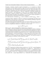
S
N
d
q
re
re
Fig. 1. Coordinates for IPMSMs
IPMSM
on d-q axis
re
Current Regulator
on axis
Current Regulator
on axis
)(⋅R
)(⋅R
1
+
ii
**
ii
qd
ii
qd

vv
vv
Fig. 2. Control system in consideration of position estimation error
3. Stability analysis of current control system
3.1 Problem Statement
This section analyses stability of current control system while considering its application to
position sensor-less system. Let γ
− δ axis be defined as a rectangular coordinate away from
d
− q axis by position error Δθ
re
shown in Fig.1. This section investigates the stability of the
current control loop, which consists of IPMSM and current controller on γ
− δ axis as shown
in Fig.2.
From (1), IPMSM on γ
−δ axis can be rewritten as

v
γ
v
δ

=

R
− Pω
rm
L
γδ

+ L
γ
p −Pω
rm
L
δ
+ L
γδ
p
Pω
rm
L
γ
+ L
γδ
pR+ Pω
rm
L
γδ
+ L
δ
p

i
γ
i
δ

+ Pω
rm

K
E

−sin Δθ
re
cos Δθ
re

, (10)
in which
L
γ
= L
d
−(L
d
− L
q
) sin
2
Δθ
re
,
L
δ
= L
q
+(L
d
− L

q
) sin
2
Δθ
re
,
L
γδ
=
L
d
− L
q
2
sin 2Δθ
re
.
It should be noted that the equivalent resistances on d axis and q axis are varied as ω
rm
increases when L
γδ
exists, which is caused by Δθ
re
.Asaresult,Δθ
re
forces us to modify the
509
Robust Current Controller Considering Position Estimation Error for Position
Sensor-less Control of Interior Permanent Magnet Synchronous Motors under High-speed Drives
current controllers (2) – (5) as follows:

v
∗
γ
= v

γ
− Pω
rm
L
q
i
δ
, (11)
v
∗
δ
= v

δ
+ Pω
rm
(L
d
i
γ
+ K
E
) , (12)
v


γ
=
K
pd
s + K
id
s
(i
∗
γ
−i
γ
) , (13)
v

δ
=
K
pq
s + K
iq
s
(i
∗
δ
−i
δ
) . (14)
3.2 Closed loop system of current control and s tability analysis
This subsection analyses robust stability of the closed loop system of current control. Consider

the robust stability of Fig.2 to Δθ
re
. Substituting the decoupling controller (11) and (12) to the
model (10) if the PWM inverter to feed the IPMSM can operate perfectly (this means v
γ
= v
∗
γ
,
v
δ
= v
∗
δ
), the following equation can be obtained:

v

γ
v

δ

=

R
− Pω
rm
L
γδ

+ L
γ
p ΔZ
γδ
(p, ω
rm
)
ΔZ
δγ
(p, ω
rm
) R + Pω
rm
L
γδ
+ L
δ
p

i
γ
i
δ

+Pω
rm
K
E

−sin Δθ

re
cos Δθ
re
−1

, (15)
where ΔZ
γδ
(p, ω
rm
) and ΔZ
δγ
(p, ω
rm
) are residual terms due to imperfect decoupling control,
and are defined as follows:
ΔZ
γδ
(p, ω
rm
)=−Pω
rm
(L
d
− L
q
) sin
2
Δθ
re

+ L
γδ
p ,
ΔZ
δγ
(p, ω
rm
)=Pω
rm
(L
d
− L
q
) sin
2
Δθ
re
+ L
γδ
p .
It sh ould be noted that the decoupling controller fails to perfectly reject coupled terms because
of Δθ
re
. In addition, with current controllers (13) and (14), the closed loop system can be
expressed as shown in Fig.3, the transfer function (16) is obtained with the assumption
pΔθ
re
= 0, pω
rm
= 0 as follows:


i
γ
i
δ

=

1 F
γδ
(s)
F
δγ
(s) 1

−1

G
γ
(s) ·i
∗
γ
G
δ
(s) ·i
∗
δ

(16)
where

F
γδ
(s)=
ΔZ
γδ
(s, ω
rm
) ·s
L
γ
s
2
+(K
pd
+ R − Pω
rm
L
γδ
)s + K
id
,
F
δγ
(s)=
ΔZ
δγ
(s, ω
rm
) ·s
L

δ
s
2
+(K
pq
+ R + Pω
rm
L
γδ
)s + K
iq
,
G
γ
(s)=
K
pd
·s + K
id
L
γ
s
2
+(K
pd
+ R − Pω
rm
L
γδ
)s + K

id
,
G
δ
(s)=
K
pq
·s + K
iq
L
δ
s
2
+(K
pq
+ R + Pω
rm
L
γδ
)s + K
iq
.
Figs.4 and 5 show step responses based on Fig.3 with conventional controller (designed with
ω
c
= 2π ×30 rad/s) at ω
rm
=500 min
−1
and 5000 min

−1
, respectively. In this simulation, Δθ
re
510
Robust Control, Theory and Applications
Fig. 3. Closed loop system of current control
Parameters Value
Rated Power 1.5 kW
Rated Speed 10000 min
−1
R 0.061 Ω
L
d
1.44 mH
L
q
2.54mH
K
E
182×10
−4
V/min
−1
P 2poles
Table 1. Parameters of test IPMSM
[
0 0.05 0.1 0.15 0.2
−1
−0.5
0

0.5
1
Time sec]
Current i
γ
[A]
(a) γ axis current response (b) δ axis current response
Fig. 4. Response with the conventional controller (ω
rm
= 500 min
−1
)
was intentionally given by Δθ
re
= −20
◦
. i
∗
δ
was stepwise set to 5 A and i
∗
γ
was stepwise kept
to the value according to maximum torque per current (MTPA) strategy:
i
∗
γ
=
K
E

2(L
q
− L
d
)
−

K
2
E
4(L
q
− L
d
)
2
+

i
∗
δ

2
. (17)
The parameters of IPMSM are shown i n Table 1. It can be seen from Fig.4 that each current can
be stably regulated to each reference. The results in Fig.5, however, illustrate that each current
diverges and fails to be successfully regulated. These results show that the current control
system tends to be unstable as the motor speed goes up. In other words, currents diverge and
511
Robust Current Controller Considering Position Estimation Error for Position

Sensor-less Control of Interior Permanent Magnet Synchronous Motors under High-speed Drives
0 0.05 0.1 0.15 0.2
0
5
10
Time [sec]
Current i [A]
0 0.05 0.1 0.15 0.2
0
2
4
6
8
10
Time [sec]
Current i [A]
(a) γ axis current response (b) δ axis current response
Fig. 5. Response with conventional controller (ω
rm
= 5000 min
−1
)
fail to be successfully regulated to each reference in high-speed region because of Δθ
re
,which
is often visible in position sensor-less control systems.
Figs.6 and 7 show poles and zero assignment of G
γ
(s) and G
δ

(s), respectively. It is revealed
from Fig.6 that all poles of G
γ
(s) and G
δ
(s) are in the left half plane, which means the
current control loop can be stabilized, and this analysis is consistent with simulation results as
previously shown. It should be noted, however, the pole by motor winding is not cancelled by
controller’s zero, since this pole moves due to Δθ
re
. On the contrary, Fig.7 shows that poles are
not in stable region. Hence stability of the current control system is violated, as demonstrated
in the aforementioned simulation. This is why one onf the equivalent resistances observed
from γ
−δ axis tends to become small as speed goes up, as s hown in (10), and poles of current
closed loop are reassigned by imperfect decoupling control.
It can be seen from G
γ
(s) and G
δ
(s) that stability criteria are given by
K
pd
+ R − Pω
rm
L
γδ
> 0 , (18)
K
pq

+ R + Pω
rm
L
γδ
> 0 . (19)
Fig.8 shows stable region by conventional current controller, which is plotted according to (18)
and (19). The figure shows that stable speed region tends to shrink as motor speed increases,
even if position error Δθ
re
is extremely small. It can also be seen that the stability condition on
γ axis (18) is more strict than that on δ axis (19) because of K
pd
< K
pq
, in which these gains
are given by (6) and (8), and L
d
< L
q
in general. To solve this instability problem, all poles of
G
γ
(s) and G
δ
(s) must be reassigned to stable region (left half plane) even if there exists Δθ
re
.
This implies that equivalent resistances in γ
−δ axis need to be increased.
4. Proposed current controller with 2DOF structure

4.1 Requirements for stable current control under high-speed region
As described previously, the stability of current control is violated by Δθ
re
.Thisisbecause
one of the equivalent resistances observed on γ
− δ axis tends to become too small, and one
of the stability criteria (18) and (19) is not satisfied under high-speed region. To enlarge the
stable region, the current controller could, theoretically, be designed with higher performance
(larger ω
c
). This strategy is, however, not consistent with the aim of achieving lower cost as
described in section 1., and thus is not a realistic solution in this case. Therefore, this instability
cannot be improved upon by the conventional PI current controller.
512
Robust Control, Theory and Applications
Imaginary Axis
Real Axis
Poles
Zero
Imaginary Axis
Real Axis
Poles
Zero
(a) G
γ
(s) (b) G
δ
(s)
Fig. 6. Poles and zero assignment of G
γ

(s) and G
δ
(s) at ω
rm
= 500 min
−1
Imaginary Axis
Real Axis
Poles
Zero
Imaginary Axis
Real Axis
Poles
Zero
(a) G
γ
(s) (b) G
δ
(s)
Fig. 7. Poles and zero assignment of G
γ
(s) and G
δ
(s) at ω
rm
= 5000 min
−1
Position Error [deg.]
Speed [min ]
-15000

-10000
-5000
0
5000
10000
15000
-40 -30 -20 -10 0 10 20 30 40
-1
Stable region
Unstable region
Unstable region
Unstable region
Unstable region
Fig. 8. Stable region by conventional current controller
513
Robust Current Controller Considering Position Estimation Error for Position
Sensor-less Control of Interior Permanent Magnet Synchronous Motors under High-speed Drives
Fig. 9. Proposed current controller with 2DOF structure (only γ axis)
On the other hand, two degree of freedom (2DOF) structure would allow us to simultaneously
determine both robust stability and its performance. In this stability improvement problem,
robust stability with respect to Δθ
re
needs to be improved up to high-speed region while
maintaining its performance, so that 2DOF structure seems to be consistent with this stability
improvement problem of current control for IPMSM drives. From this point of view, this paper
employees 2DOF structure in the current controller to enlarge the stability region.
4.2 Proposed current controller
The following equation describes the proposed current controller:
v


γ
=
K
pd
s + K
id
s
(i
∗
γ
−i
γ
) −K
rd
i
γ
, (20)
v

δ
=
K
pq
s + K
iq
s
(i
∗
δ
−i

δ
) −K
rq
i
δ
. (21)
Fig. 9 illustrates the block diagram of the proposed current controller with 2DOF structure,
whereitshouldbenotedthatK
rd
and K
rq
are just added, compared with the conventional
current controller. This current controller consists of conventional decoupling controllers (11)
and (12), conventional PI controllers with current control error (13) and (14) and the additional
gain on γ
− δ axis to enlarge stable region. Hence, this controller seems to be very simple for
its implementation.
4.3 Closed loop system using proposed 2DOF controller
Substituting the decoupling controller (11) and (12), and the proposed current controller with
2DOF structure (20) and (21) to the model (10), the following closed loop system can be
obtained:

i
γ
i
δ

=

1 F


γδ
(s)
F

δγ
(s) 1

−1

G

γ
(s) ·i
∗
γ
G

δ
(s) ·i
∗
δ

514
Robust Control, Theory and Applications
Fig. 10. Current control system with K
rd
and K
rq
where

F

γδ
(s)=
ΔZ
γδ
(s, ω
rm
) ·s
L
γ
s
2
+(K
pd
+ K
rd
+ R −Pω
rm
L
γδ
)s + K
id
,
F

δγ
(s)=
ΔZ
δγ

(s, ω
rm
) ·s
L
δ
s
2
+(K
pq
+ L
rq
+ R + Pω
rm
L
γδ
)s + K
iq
,
G

γ
(s)=
K
pd
·s + K
id
L
γ
s
2

+(K
pd
+ K
rd
+ R −Pω
rm
L
γδ
)s + K
id
,
G

δ
(s)=
K
pq
·s + K
iq
L
δ
s
2
+(K
pq
+ K
rq
+ R + Pω
rm
L

γδ
)s + K
iq
.
From these equations, stability criteria are given by
K
pd
+ K
rd
+ R −Pω
rm
L
γδ
> 0 , (22)
K
pq
+ K
rq
+ R + Pω
rm
L
γδ
> 0 . (23)
The effect of K
rd
and K
rq
is described here. It should be noted from stability criteria (22) and
(23) that these gains are injected in the same manner as resistance R, so that the current control
loop system with K

rd
and K
rq
is depicted by Fig.10. This implies that K
rd
and K
rq
play a role
in virtually increasing the stator resistance of IPMSM. In other words, the poles assigned near
imaginary axis (
= −
R
L
d
, −
R
L
q
)aremovedtotheleft(= −
R+K
rd
L
d
, −
R+K
rq
L
q
) by proposed current
controller, which means that robust current control can be easily realized by designers. In

the proposed current controller, PI gains are selected in the same manner as occur in the
conventional design:
K
pd
= ω
c
L
d
, (24)
K
id
= ω
c
(R + K
rd
) , (25)
K
pq
= ω
c
L
q
, (26)
K
iq
= ω
c
(R + K
rq
) . (27)

This parameter design makes it possible to cancel one of re-assigned poles by zero of PI
controller when Δθ
re
= 0
◦
. It should be noted, based this design, that the closed loop dynamics
515
Robust Current Controller Considering Position Estimation Error for Position
Sensor-less Control of Interior Permanent Magnet Synchronous Motors under High-speed Drives
by the proposed controller is identical to that by conventional controller r egardless of K
rd
and
K
rq
:
i
d
i
∗
d
=
i
q
i
∗
q
=
ω
c
s + ω

c
.
Therefore, the proposed design can improve robust stability by only proportional gains K
rd
and K
rq
while maintaining closed loop dynamics of the current control. This is why the
authors have chosen to adopt 2DOF control.
4.4 Design of K
rd
and K
rq
, and pole re-assignment results
As previously described, re-assigned poles by proposed controller (= −
R+K
rd
L
d
, −
R+K
rq
L
q
)can
further be moved to the left in the s
−plane as larger K
rd
and K
rq
are designed. However,

employment of lower-performance micro-processor is considered in this paper as described
in section 1., and re-assignment of poles by K
rd
and K
rq
is restricted to the cut-off frequency of
the closed-loop dynamics at most. Hence, K
rd
and K
rq
design must satisfy
R
+ K
rd
L
d
≤ ω
c
, (28)
R
+ K
rq
L
q
≤ ω
c
. (29)
As a result, the design of additional gains is proposed as follows:
K
rd

= −R + ω
c
L
d
, (30)
K
rq
= −R + ω
c
L
q
. (31)
Based on this design, characteristics equation of the proposed current closed loop (the
denominator of G

γ
(s) and G

δ
(s) ) is expressed under Δθ
re
= 0by
Ls
2
+ 2ω
c
Ls + ω
2
c
L = 0,

where L stands for L
d
or L
q
. This equation implies that the dual pole assignment at s = −ω
c
is the most desirable solution to improve robust stability with respect to Δθ
re
under the
restriction of ω
c
. In other words, this design can guarantee stable poles in the left half plane
even if the poles move from the specified assignment due to Δθ
re
.
4.5 Stability analysis using proposed 2DOF controller
Fig.11 shows stable region according to (22) and (23) by proposed current controller designed
with ω
c
= 2π × 30 rad/s. It should be noted from these results that the stable speed region
can successfully be enlarged up to high-speed range compared with conventional current
regulator(dashed lines), which is the same in Fig. 8. Point P in this figure stands for operation
point at ω
rm
=5000 min
−1
and Δθ
re
= −20
◦

. It can be seen from this stability map that
operation point P can be stabilized by the proposed current controller with 2DOF structure,
despite the fact that the conventional current regulator fails to realize stable control and
current diverges, as shown in the previous step response.
Fig.12 demonstrates that stable step response can be realized under ω
rm
=5000 min
−1
and
Δθ
re
= −20
◦
. These results demonstrate that robust current control can experimentally be
realized even if position estimation error Δθ
re
occurs in position sensor-less control.
516
Robust Control, Theory and Applications
-15000
-10000
-5000
0
5000
10000
15000
-40 -30 -20 -10 0 10 20 30 40
Position Error [deg.]
Stable region
by proposed controller

Unstable region
Unstable region
Speed [min ]
-1
Unstable region
Unstable region
P
Fig. 11. Stable region by the proposed current regulator with 2DOF structure
(a) γ axis current response (b) δ axis current response
Fig. 12. Response with proposed controller (ω
rm
= 5000 min
−1
)
5. Experimental results
5.1 System setup
Experiments were carried out to confirm the effectiveness of the proposed design. The
experimental setup shown in Fig.13 consists of a tested IPMSM (1.5 kW) with concentrated
winding, a PWM inverter with FPGA and DSP for implementation of vector controller, and
position estimator. Also, the induction motor was utilized for load regulation. Parameters
of the test IPMSM are shown in Table 1. The speed controller, the current controller, and
the coordinate transformer were executed by DSP(TI:TMS320C6701), and the pulse width
modulation of the voltage reference was made by FPGA(Altera:EPF10K20TC144-4). The
estimation period and the control period were 100 μs, which was set relatively short to
experimentally evaluate the analytical results discussed in continuous time domain. The
carrier frequency of the PWM inverter was 10 kHz. Also, the motor currents were detected
by 14bit ADC. Rotor position was measured by an optical pulse encoder(2048 pulse/rev).
517
Robust Current Controller Considering Position Estimation Error for Position
Sensor-less Control of Interior Permanent Magnet Synchronous Motors under High-speed Drives

14bit
A/D
14bit
A/D
COUNTER
PE
IPMSM
LATCH
INVERTER
DRIVER
PWM
Pattern
Dead Time
FPGA
3φ
AC200[V]
θ
re
i
v
TMS320C6701
DSP
LEAD LAG
TMS320C6701 SYSTEM BUS
FPGA
v
*
Fig. 13. Configuration of system setup
5.2 Robust stability of current control to rotor position error
The first experiment demonstrates robust stability of the proposed 2DOF controller. In

this experiment, the test IPMSM speed was controlled using vector control with position
detection in speed regulation mode. The load was kept constant to 75% motoring torque by
vector-controlled induction motor. In order to evaluate robustness to rotor position error, Δθ
re
was intentionally given from 0
◦
to −45
◦
gradually in these experiments.
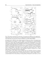
Figs. 1 4 and 15 show current c ontrol results of the conventional PI controller a nd the proposed
2DOF controller (ω
c
= 200rad/s) at 4500min
−1
, respectively. It is obvious from Fig.14 that
currents started to be violated at 3.4sec, and they finally were interrupted by PWM inverter
due to over-current at 4.2sec. These experimental results showed that Δθ
re
where currents
started to be violated was about -21
◦
, which is consistent with (18) and (19). On the other
hand, the proposed 2DOF controller can robustly stabilize current control despite large Δθ
re
as shown in Fig.15. This result is also consistent with the robust stability analysis discussed
in the previous section. Although a current ripple is steadily visible in both experiments, we
confirmed that this ripple is primarily the 6th-order component of rotor speed. The tested
IPMSM was constructed with concentrated winding, and this 6th-order component cannot be
suppressed by lower-performance current controller.
Experimental results at 7000min

−1
are illustrated in Figs.16 and 17. In the case of conventional
controller, current control system became unstable at Δθ
re
= −10
◦
as shown in Fig.16. Fig.17
shows results of the proposed 2DOF controller, in which currents were also tripped at Δθ
re
=
−
21
◦
.AllΔθ
re
to show unstable phenomenon is met to (18) and (19), which describes that
the robust stability analysis discussed in the previous section is theoretically feasible. This
robust stability cannot be improved upon as far as the proposed strategy is applied. In other
words, furthermore robust stability improvement necessitates higher cut-off frequency ω
c
,
which forces us to employ high-performance processor.
5.3 Position sensor-less control
This subsection demonstrates robust stability of current control system when position
sensor-less control is applied. As the method for p osition estimation, the disturbance observer
based on the extended electromotive force model ( Z.Chen et al. (2003) ) was utilized for
all experiments. Rotor speed estimation was substituted by differential value of estimated
518
Robust Control, Theory and Applications
sec1

*
δ
i
δ
i
γ
i
o
40
1
min4000
−
o
0
1
min0
−
A0
A0
re
θΔ
A0
A8
rm
ω
sec1
*
δ
i
δ

i
γ
i
o
40
1
min4000
−
o
0
1
min0
−
A0
A0
re
θΔ
A0
A8
rm
ω
Fig. 14. Current control characteristics by conventional controller at 4500min
−1
δ
δ
γ
Fig. 15. Current control characteristics by proposed controller at 4500min
−1
δ
δ

γ
Fig. 16. Current control characteristics by conventional controller at 7000min
−1
δ
δ
γ
Fig. 17. Current control characteristics by proposed controller at 7000min
−1
519
Robust Current Controller Considering Position Estimation Error for Position
Sensor-less Control of Interior Permanent Magnet Synchronous Motors under High-speed Drives
δ
δ
γ
Fig. 18. Current control characteristics by position sensor-less system with conventional
controller
sec0.2
q
i
i
i
1
min4000
−
o
0
1
min0
−
A0

A0
re
θΔ
A0
A8
rm
ω
o
40
sec0.2
*
i
i
i
1
min4000
−
o
0
1
min0
−
A0
A0
re
θΔ
A0
A8
rm
ω

o
40
o
40
δ
δ
γ
Fig. 19. Current control characteristics by position sensor-less system with proposed
controller
rotor position. It should be noted, however, that position estimation delay n ever fails to o ccur,
especially under high-speed drives, due to the low-pass filter constructed in the disturbance
observer. This motivated us to investigate robustness of current control to position estimation
delay.
5.3.1 Current step response in position sensor-less control
Figs.18 and 19 show current control results with conventional PI current controller and the
proposed controller(designed with ω
c
= 300rad/s), respectively. In these experiments, rotor
speed was kept to 7000min
−1
by the induction motor.
It turns out from Fig.18 that currents showed over-current i mmediately after current reference
i
∗
q
changed from 1A to 5A, and PWM inverter finally failed to flow the current to the test
IPMSM. On the contrary, Fig.19 illustrates that stable current response can be realized even
when the current reference is stepwise, which means that the proposed controller is superior
to the conventional one in terms of robustness to Δθ
re

.
Also, these figures show that Δθ
re
of about − 40
◦
is steadily caused because of estimation
delay in disturbance observer. Needless to say, this error can be compensated since DC
component of Δθ
re
can be obtained in advance according to motor speed and LPF time
constant in disturbance observer. Δθ
re
cannot be compensated, however, at the transient time.
520
Robust Control, Theory and Applications
sec0.5
*
i
i
i
1
min4000
−
o
0
1
min0
−
A0
A0

re
θΔ
A0
A8
rm
ω
o
40
o
40
δ
δ
γ
Fig. 20. Speed control characteristics by position sensor-less system with conventional
controller
δ
δ
γ
Fig. 21. Speed control characteristics by position sensor-less system with proposed controller
In this study, the authors aimed for robust stability improvement to position estimation error
in consideration of transient characteristics such as speed step response and current step
response. Hence, Δθ
re
was not corrected intentionally in these experiments.
5.3.2 Speed step response in position sensor-less control
Figs.20 and 21 show speed step response from ω
∗
rm
= 2000min
−1

to 6500min
−1
by the
conventional PI current controller and proposed controller(designed with ω
c
= 200rad/s),
respectively. 20% motoring load was given by the induction motor in these experiments.
It turns out from Fig. 20 that current control begins to oscillate at 0.7sec due to Δθ
re
,and
then the amplitude of current oscillation increases as speed goes up. On the other hand, the
proposed current controller (Fig. 21) makes it possible to realize stable step response with the
assistance of the robust current controller to Δθ
re
.
It should be noted that these experimental results were obtained by the same sensor-less
control system except with a dditional gain and its design of the proposed current controller.
Therefore, these sensor-less control results show that robust current controller enables us to
improve performances of t otal control system, and it is important to design robust current
controller to Δθ
re
as well as to re alize precise position estimation, which has been surveyed by
many researchers over several decades.
521
Robust Current Controller Considering Position Estimation Error for Position
Sensor-less Control of Interior Permanent Magnet Synchronous Motors under High-speed Drives
6. Conclusions
This paper is summarized as follows:
1. Stability analysis has been carried out while considering its application to position
sensor-less system, and operation within stable region by conventional current controller

has been analyzed. As a result, this paper has clarified that current control system tends to
become unstable as motor speed goes up due to position estimation error.
2. This paper has proposed a new current controller. To guarantee both robust stability and
performance of current control simultaneously, two degree of freedom (2DOF) structure
has been utilized in the current controller. In addition, a design of proposed controller has
also been proposed, that indicated the most robust controller could be realized under the
restriction of lower-performance processor, and thus clarifying the limitations of robust
performance.
3. Some experiments have shown the feasibility of the proposed current controller with 2DOF
structure to realize an enlarged stable region and to maintain its performance.
This paper clarifies that robust current controller enables to improve performances of total
control system, and it is important to design robust current controller to Δθ
re
as well as to
realize precise position estimation.
7.References
Hasegawa, M., Y.Mizuno & K.Matsui (2007). Robust current controller for ipmsm high speed
sensorless drives, Proc. of Power Conversion Conference 2007 pp. 1624 –1629.
J.Jung & K.Nam (1999). A Dynamic Decoupling Control Scheme for High-Speed Operation of
Induction Motors, IEEE Trans. on Industrial Electronics 46(1): 100 – 110.
K.Kondo, K.Matsuoka & Y.Nakazawa (1998 (in Japanese)). A Designing Method in Current
Control System of Permanent Magnet Synchronous Motor for Railway Vehicle, IEEJ
Trans. on Industry Applications 118-D(7/8): 900 – 907.
K.Tobari, T.Endo, Y.Iwaji & Y.Ito (2004 (in Japanese)). Stability Analysis of Cascade Connected
Vector Controller for High-Speed PMSM Drives, Proc. of the 2004 Japan Industry
Applications Society Conference pp. I.171–I.174.
M.Hasegawa & K.Matsui (2008). IPMSM Position Sensorless Drives Using Robust Adaptive
Observer on Stationary Reference Frame, IEEJ Transactions on Electrical and Electronic
Engineering 3(1): 120 – 127.
S.Morimoto, K.Kawamoto, M.Sanada & Y.Takeda (2002). Sensorless Control Strategy for

Salient-pole PMSM Based on Extended EMF in Rotating Reference Frame, IEEE
Trans. on on Industry Applications 38(4): 1054 – 1061.
Z.Chen, M.Tomita, S.Doki & S.Okuma (2003). An Extended Electromotive Force Model for
Sensorless Control of Interior Permanent-Magnet Synchronous Motors, IEEE Trans.
on Industrial Electronics 50(2): 288 – 295.
522
Robust Control, Theory and Applications
João Marcos Kanieski
1,2,3
, Hilton Abílio Gründling
2
and Rafael Cardoso
3
1
Embrasul Electronic Industry
2
Federal University of Santa Maria - UFSM
3
Federal University of Technology - Paraná - UTFPR
Brazil
1. Introduction
The most common approach to design active power filters and its controllers is to consider
the plant to be controlled as the coupling filter of the active power filter. The load dynamics
and the line impedances are usually neglected and considered as perturbations in the
mathematical model of the plant. Thus, the controller must be able to reject these perturbations
and provide an adequate dynamic behavior for the active power filter. However, depending
on these perturbations the overall system can present oscillations and even instability. These
effects have been reported in literature (Akagi, 1997), (Sangwongwanich & Khositkasame,
1997), (Malesani et al., 1998). The side effects of the oscillations and instability are evident in
damages to the bank of capacitors, frequent firing of protections and damage to line isolation,

among others (Escobar et al., 2008).
Another problem imposed by the line impedance is the voltage distortion due the circulation
of non-sinusoidal current. It degrades the performance of the active power filters due its
effects on the control and synchronization systems involved. The synchronization problem
under non-sinusoidal voltages can be verified in (Cardoso & Gründling, 2009). The line
impedance also interacts with the switch commutations that are responsible for the high
frequency voltage ripple at the point of common coupling (PCC) as presented in (Casadei
et al., 2000).
Due the effects that line impedance has on the shunt active filters, several authors have been
working on its identification or on developing controllers that are able to cope with its side
effects. The injection of a small current disturbance is used in (Palethorpe et al., 2000) and
(Sumner et al., 2002) to estimate the line impedance. A similar approach, with the aid of
Wavelet Tranform is used in (Sumner et al., 2006). Due to line impedance voltage distortion,
(George & Agarwal, 2002) proposed a technique based on Lagrange multipliers to optimize
the power factor while the harmonic limits are satisfied. A controller designed to reduce the
perturbation caused by the mains voltage in the model of the active power filter is introduced
in (Valdez et al., 2008). In this case, the line impedances are not identified. The approach is
intended to guarantee that the controller is capable to reject the mains perturbation.
Therefore, the line impedances are a concern for the active power filters designers. As shown,
some authors choose to measure (estimate or identify) the impedances. Other authors prefer
Robust Algorithms Applied for Shunt Power
Quality Conditioning Devices
24
to deal with this problem by using an adequate controller that can cope with this uncertainty
or perturbation. In this chapter the authors use the second approach. It is employed a Robust
Model Reference Adaptive Controller and a fixed Linear Quadratic Regulator with a new
mathematical model which inserts robustness to the system. The new LQR control scheme
uses the measurement of the common coupling point voltages to generate all the additional
information needed and no disturbance current is used in this technique.
2. Model of the plant

The schematic diagram of the power quality conditioning device, consisting of a DC source
of energy and a three-phase/three-legs voltage source PWM inverter, connected in parallel to
the utility, is presented in Fig 1.
Fig. 1. Schematic diagram of the power quality conditioning device.
The Kirchoff’s laws for voltage and current, applied at the PCC, allow us to write the 3
following differential equations in the ”123” frame,
v
1N
= L
f
di
F1
dt
+ R
f
i
F1
+ v
1M
+ v
MN
, (1)
v
2N
= L
f
di
F2
dt
+ R

f
i
F2
+ v
2M
+ v
MN
, (2)
v
3N
= L
f
di
F3
dt
+ R
f
i
F3
+ v
3M
+ v
MN
. (3)
The state space variables in the ”123” frame have sinusoidal waveforms in steady state. In
order to facilitate the control efforts of this system, the model may be transformed to the
rotating reference frame ”dq”. Such frame changing is made by the Park’s transformation,
given by (4).
C
123

dqO
=
2
3
⎡
⎢
⎢
⎣
sin
(
ωt
)
sin

ωt −
2π
3

sin

ωt
−
4π
3

cos
(
ωt
)
cos


ωt −
2π
3

cos

ωt
−
4π
3

3
2
3
2
3
2
⎤
⎥
⎥
⎦
. (4)
524
Robust Control, Theory and Applications
The state space variables represented in the ’dq’ frame are related to the ”123” frame state
space variables by equations (5)-(7).

v
d

v
q
v
O

T
= C
123
dqO

v
1
v
2
v
3

T
, (5)

i
d
i
q
i
O

T
= C
123

dqO

i
1
i
2
i
3

T
, (6)

d
d
d
q
d
O

T
= C
123
dqO

d
1
d
2
d
3


T
. (7)
The inverse process is given in equations (8)-(10),

v
1
v
2
v
3

T
= C
dqO
123

v
d
v
q
v
O

T
, (8)

i
1
i

2
i
3

T
= C
dqO
123

i
d
i
q
i
O

T
, (9)

d
1
d
2
d
3

T
= C
dqO
123


d
d
d
q
d
O

T
, (10)
where,
C
dqO
123
= C
123
dqO
−1
=
3
2
C
123
dqO
T
, (11)
and d is the switching function (Kedjar & Al-Haddad, 2009). As it is a three-phase/three-wire
system, the zero component of the rotating frame is always zero, thus the minimum plant
model is then given by Eq. (12)
d

dt

i
dq

= A

i
dq

+ B

d
dq

+ E

v
dq

, (12)
where,
A
= −
⎡
⎣
R
f
L
f

−ω
ω
R
f
L
f
⎤
⎦
, B
= −

v
dc
L
f
0
0
v
dc
L
f

,
E
=

1
L
f
0

0
1
L
f

and C
=

10
01

.
Eq. (12) shows the direct system state variable dependency on the voltages at the PCC, which
are presented in the ’dq’ frame (v
dq
). Fig. 2 depicts the plant according to that representation.
Based on the block diagram of Fig. 2, it can be seen that the voltages at the PCC have direct
influence on the plant output. It suggests that the control designer has also to be careful with
those signals, which are frequently disregarded on the project stage.
2.1 Influence of the line impedance on the grid voltages
In power conditioning systems’ environment, the line impedance is often an unknown
parameter. Moreover, it has a strong impact on the voltages at the PCC, which has its harmonic
content more dependent on the load, as the grid impedance increases. Fig. 3 shows the open
loop system with a three-phase rectified load connected to the grid through a variable line
impedance.
As already mentioned, by increasing the line impedance values, the harmonic content of the
voltages at the PCC also increases. Higher harmonic content in the voltages leads to a more
525
Robust Algorithms Applied for Shunt Power Quality Conditioning Devices
Fig. 2. Block representation of the plant.

Fig. 3. Open loop system with variable line inductance
distorted waveform. It can be visualized in Fig. 4, that shows the voltage signals v
123
at the
PCC, for a line inductance of L
S
= 2mH.
Fig. 4. Open loop voltages at the PCC with line inductance of L
S
= 2mH.
526
Robust Control, Theory and Applications
Fig. 5 shows now an extreme case, with line inductance of L
S
= 5mH, it is also visually
perceptible the significant growth on the voltage harmonic content.
Fig. 5. Open loop voltages at the PCC with line inductance of L
S
= 5mH.
Concluding, the voltages at the PCC have its dynamic substantially dependent on the line
impedance. In other hand, the system dynamic is directly associated with the PCC voltages.
Therefore, the control of this kind of system strongly depends on the behavior of the voltages
at the PCC. As the output filter of the Voltage Source Inverter (VSI) has generally well-known
parameters (they are defined by the designer), which are at most fixed for the linear system
operation, one of the greatest control challenges of these plants is associated with the PCC
voltages. The text that follows is centered on that point and proposes an adaptive and a fixed
robust algorithm in order to control the chosen power conditioner device, even under load
unbalance and line with variable or unknown impedance.
3. Robust Model Reference Adaptive Control (RMRAC)
The RMRAC controller has the characteristic of being designed under an incomplete

knowledge of the plant. To design such controller it is necessary to obtain a representative
mathematical model for the system. The RMRAC considers in its formulation a parametric
model with a reduced order modeled part, as well as a multiplicative and an additive term,
describing the unmodeled dynamics. The adaptive law is computed for compensating the
plant parametric variation and the control strategy is robust to such unmodeled dynamics. In
the present application, the uncertainties are due to the variation of the line impedance and
load.
3.1 Mathematical model
From the theory presented by Ioannou & Tsakalis (1986) and by Ioannou & Sun (1995), to have
an appropriated RMRAC design, the plant should be modeled in the form
i
F
(s)
u(s)
=
G( s)=G
0
(s)[1 + μΔ
m
(s)] + μΔ
a
(s)
G
0
(s)=k
p
Z
0
(s)
R

0
(s)
(13)
where u represents the control input of the system and i
F
is the output variable of interest as
shown in Fig. 1.
527
Robust Algorithms Applied for Shunt Power Quality Conditioning Devices
⇒ Assumptions for the Plant
H1.Z
0
is a monic stable polynomial of degree m(m ≤ n −1),
H2.R
0
is a monic polynomial of degree n;
H3.The sign of k
p
> 0 and the values of m, n are known.
For the unmodeled part of the plant it is assumed that:
H4.Δ
m
is a stable transfer function;
H5.Δ
a
is a stable and strictly proper transfer function;
H6.A lower bound p
0
> 0 on the stability margin p > 0 for which the poles of Δ
m

(s − p) and
Δ
a
(s − p) are stable is known.
3.2 RMRAC strategy
The goal of the model reference adaptive control can be summarized as follows: Given a
reference model
y
m
r
= W
m
(s)=k
m
Z
m
(s)
R
m
(s)
, (14)
it is desired to design an adaptive controller, for μ
> 0 and μ ∈
[
0, μ
∗
)
where the resultant
closed loop system is stable and the plant output tracks, as closer as possible, the model
reference output, even under the unmodeled dynamics Δ

m
and Δ
a
. In (14), r is a uniformly
limited signal.
⇒ Assumptions for the model reference:
M1.Z
m
a monic stable polynomial of degree m(m ≤ n −1);
M2.R
m
is a monic polynomial of degree n.
The plant input is given by
u
=
θ
T
ω + c
0
r
θ
4
(15)
where θ
T
=

θ
T
1

, θ
T
2
, θ
3

, ω
T
=
[
ω
1
, ω
2
, y
]
∈
2n−1
and c
0
is the relation between the gain
of the open loop system and the gain of the model reference. The input u and the plant output
y are used to generate the signals ω
1
, ω
2
∈
n− 1
ω
1

=
α( s)
Λ(s)
u and ω
2
=
α( s)
Λ(s)
y. (16)
⇒ Assumptions for the signals ω
1
and ω
2
:
R1.The polynomial Λ in (16) is a monic Hurwitz of degree n
−1, containing stable eigenvalues.
R2.For n
≥ 2, α 

s
n− 2
, , s,1

T
and for n = 1, α  0.
For the adaptation of the control action parameters, the following modified gradient algorithm
was considered
˙
θ
= −σPθ−

Pζε
m
2
(17)
528
Robust Control, Theory and Applications
The σ-modification in 17 is given by
σ
=
⎧
⎪
⎪
⎨
⎪
⎪
⎩
0if

θ

<
M
0
σ
0


θ

M

0
−1

if M
0
≤

θ

<
2M
0
σ
0
if

θ

>
2M
0
(18)
where σ
0
> 0 is a parameter of design. P = P
T
> 0, ε = y − y
m
+ θ
T

ζ − W
m
ν = φ
T
ζ + μη
and M
0
is an upper limit θ
∗
, such that θ
∗
 + δ
3
≤ M
0
for a δ
3
> 0. The normalization
signal m is given by
˙
m
= −δ
0
m + δ
1
(
|
u| + |y| + 1
)
(19)

with m
0
> δ
1
/δ
0
, δ
1
≥ 1 and δ
0
> 0.
The normalization signal m is the parameter which ensures the robustness of the system.
Looking to Eq. (15)-(19), it can be seen that when the control action u, the plant output y or
both variables are large enough, the θ parameters decreases and therefore the control action,
which depends on the θ parameters, also has its values reduced, limiting the control action as
well as the system output in order to stabilize the system.
3.3 RMRAC applied for the power conditioning device
In the considered power conditioning system, as shows Eq. (12), there is a coupling between
the "dq" variables. To facilitate the control strategy, which should consider a multiple input
multiple output system (MIMO), it is possible to rewrite Eq. (12) as
L
f
di
d
dt
+ R
f
i
d
= L

f
ωi
q
−v
dc
d
nd
+ v
d
L
f
di
q
dt
+ R
f
i
q
= −L
f
ωi
d
−v
dc
d
nq
+ v
q
(20)
Defining, the equivalent input as in Eq. (21) and (22),

u
d
= L
f
ωi
q
−v
dc
d
nd
+ v
d
(21)
and
u
q
= −L
f
ωi
d
−v
dc
d
nq
+ v
q
, (22)
the MIMO tracking problem, with coupled dynamics, is transformed in two single input single
output (SISO) problems, with decoupled dynamics. Thus, currents i
d

and i
q
may be controlled
independently through the inputs u
d
e u
q
, respectively. For the presented decoupled plant, the
RMRAC controller equations are given by (23) and (24).
u
d
=
θ
T
d
ω
d
+ c
0
r
d
θ
4d
(23)
and
u
q
=
θ
T

q
ω
q
+ c
0
r
q
θ
4q
. (24)
The PWM actions (d
nd
and d
nq
), are obtained through Eq. (21) and (22) after computation of
(23) and (24).
529
Robust Algorithms Applied for Shunt Power Quality Conditioning Devices
3.3.1 Design procedure
Before starting the procedure, lets examine the hypothesis H1, H2, M1, M2, R1 and R2. Firstly,
as the nominal system, accordingly to Eq. (12), is a first order plant. The degrees n and m are
then defined by n
= 1 and m = 0. Therefore, the structure of the model reference and the
dynamic of signals ω
1
and ω
2
can be determined. By M1 and M2, the model reference is also
a first order transfer function W
m

(s), thus
W
m
(s)=k
m
ω
m
s −ω
m
. (25)
Furthermore, from R1 and R2: α
 0; and from Eq. (15), the control law reduces to
u
d
=
θ
3d
i
d
+ r
d
θ
4d
(26)
and
u
q
=
θ
3q

i
q
+ r
q
θ
4q
. (27)
From the information of the maximum order harmonic, which has to be compensated by
the power conditioning device, it is possible to design the model reference, given in Eq. 25.
Choosing, for example, the 35
th
harmonic, as the last harmonic to be compensated, and W
m
(s)
with unitary gain, the model reference parameters become ω
m
= 35 ·2 ·π ·60 ≈ 13195
rad
s
and
k
m
= 1. Fig. 6 shows the frequency responses of the nominal plant of a power conditioning
device, with parameters L
f
= 1mH and R
f
= 0.01Ω and of a model reference with the
parameters aforementioned.
Fig. 6. Bode diagram of G

0
(s) and W
m
(s).
The vector θ is obtained by the solution of a Model Reference Controller (MRC) for the
modeled part of the plant G
0
(s). The design procedure of a MRC is basically to calculate the
closed loop system of the nominal plant which has to be equal to the model reference transfer
function.
530
Robust Control, Theory and Applications
3.3.2 RMRAC results
The RMRAC was applied to the power conditioning device, shown in Fig. 7, to control the
compensation currents i
F123
. Table 1 summarizes the parameters of the system.
Fig. 7. Block diagram of the system.
Grid Voltage 380V (RMS) R
f
0.01Ω
ω 377rad/sL
f
1mH
f
s
12kHz R
S
0.01Ω
V

dc
550VL
S
5uH /2mH /5mH
θ
d
(0)[−1.02, 0.53]
T
P diag{0.99, 0.99}
θ
q
(0)[−1.02, 0.53]
T
k
m
1
c
0
1 ω
m
13195
rad
s
L
L
2mH L
L1
2mH
R
L

25Ω R
L1
25Ω
Table 1. Design Parameters
To verify the robustness of the closed loop system, which has to be stable for an appropriated
range of line inductance (in the studied case: from L
S
= 5μH to L
S
= 5mH), some simulations
were carried out considering variations on the line inductance (L
S
).
In the first analysis, it was considered a line impedance of L
S
= 5uH. Fig. 8 (a) shows the load
currents as well as the compensated currents, which are provided by the main source. It is
also possible to see by Fig. 8 (b) the appropriate reference tracking for the RMRAC controlled
system for the case of small line inductance. Fig 8 (b) shows the reference currents in black
plotted with the compensation currents in gray.
531
Robust Algorithms Applied for Shunt Power Quality Conditioning Devices