Ultra Wideband Communications Novel Trends System, Architecture and Implementation Part 11 potx
Bạn đang xem bản rút gọn của tài liệu. Xem và tải ngay bản đầy đủ của tài liệu tại đây (1.06 MB, 25 trang )
A Method for Improving Out-Of-Band Characteristics
of a Wideband Bandpass Filter in an LTCC Substrate
239
C
a1
0.27pF Z
S1
46.3 ohm Z
So
45.7 ohm
2S
θ
10 deg.
C
a2
0.25pF Z
Se
45.9 ohm
1S
θ
18 deg.
3S
θ
5 deg.
Table 2. Parameters of the lowpass filters shown in Fig.7.
Fig. 8. Simulated results of the filter shown in Fig.7.
Fig. 9. Simulated results of the filter shown in Fig.7, when the coupling condition of the
stripline is varied.
Ultra Wideband Communications: Novel Trends – System, Architecture and Implementation
240
4. LTCC structure
Fig.10, Fig.11 and Fig.12 indicate the LTCC structure of the filter. The filter is obtained by
means of modifying the structure based on the basic circuit shown in Fig.7, taking into
consideration the various parasitic effects caused by the three-dimensional LTCC structure.
The filter consists of the three conductor layers inserted into the middle portion of the LTCC
substrate, with the ground planes on the top and bottom layers. The conductor thickness is 8
um. The diameter of via holes is 0.1 mm. The ground planes are connected by the via holes.
The via hole between the coupled line adjusts the coupling condition. The dimensions of the
bandpass filter are 6.2 x 2.7 x 0.366 mm
3
, and this size could be fabricated into the LTCC
substrate for wireless modules. Fig.13 shows the simulated results using a commercial
electromagnetic simulator (HFSS Ansys Inc.). The filter has the wide passband and
suppresses second and third harmonics. The filter also has an additional attenuation pole at
the low-frequency region.
Fig. 10. Three-dimensional structure of the filter.
Fig. 11. Cross sectional structure of the filter.
A Method for Improving Out-Of-Band Characteristics
of a Wideband Bandpass Filter in an LTCC Substrate
241
Fig. 12. Top view of the filter.
Ultra Wideband Communications: Novel Trends – System, Architecture and Implementation
242
Fig. 13. Simulated results by the electromagnetic simulator.
5. Experiments
We verify the effectiveness of the presented method by experiments. Fig. 14 indicates the
LTCC structure for the evaluation of the embedded filter. The dimensions of the LTCC
Fig. 14. Structure of the LTCC substrate for evaluation.
A Method for Improving Out-Of-Band Characteristics
of a Wideband Bandpass Filter in an LTCC Substrate
243
substrate are 8.0 x 5.0 x 0.63 mm
3
. The presented filter (6.2 x 2.7 x 0.366 mm
3
) is fabricated in
the substrate. In order to connect the SMA connectors for the evaluation, the top layer of the
LTCC substrate has the electrodes for RF signals and a ground plane. The feed lines between
the filter and the input/output ports consist of a via hole, a stripline, and the electrode of the
top layer. These feed lines are designed 50 ohm. Fig. 15 shows a photograph of the LTCC
substrate. The prototype which is connected to the SMA connectors is measured by a vector
network analyzer (N5230A PNA-L, Agilent Technologies Inc). Fig.16 and Fig.17 indicate the
measured results. It is confirmed that the filter suppresses the spurious responses less than
20 dB up to 16 GHz and has an additional attenuation pole in the low-frequency region. In
addition, the insertion loss is less than 3.0dB and the group delay is within 1 ns in the wide
passband.
Fig. 15. Photograph of the prototype.
Ultra Wideband Communications: Novel Trends – System, Architecture and Implementation
244
Fig. 16. Measured results of the filter shown in Fig.15.
Fig. 17. Measured group delay of the filter shown in Fig.15.
A Method for Improving Out-Of-Band Characteristics
of a Wideband Bandpass Filter in an LTCC Substrate
245
6. Conclusion
In this study, we propose a method for improving out-of-band characteristics for the
wideband filter in the LTCC substrate. This method uses the lowpass filters with the
coupling structure, which are set at input and output ports of the bandpass filter. This
method is very useful for the compact wireless modules because additional compact circuits
can suppress spurious responses and can add an attenuation pole in the low-frequency
band. The fabricated UWB bandpass filter for the low-frequency band achieves the insertion
loss less than 3.0 dB and the group delay within 1 ns in the wide passband. The filter also
suppresses spurious responses up to 16 GHz and has the good attenuation performances in
the low-frequency region.
7. References
Lin, Y S., Liu, C C., Li,K M., & Chen, C.H. (2004). Design of an LTCC tri-band transceiver
module for GPRS mobile applications.
IEEE Transactions on Microwave Theory and
Techniques
, Vol. 52, No. 12, pp. 2718-2724.
Wang, G., Van, M., Barlow, F. & Elshabini, A. (2005). An interdigital bandpass filter
embedded in LTCC for 5- GHz wireless LAN applications.
IEEE Microwave and
Wireless Components Letters,Vol. 15, No. 5, pp. 357-359.
Ishida, H. & Araki, K. (2004). Design and analysis of UWB bandpass filter with ring filter.
IEEE MTT-S International Microwave Symposium, pp. 1307-1310.
Saitou, A., Aoki, H. , Satomi, N., Honjo, K., Sato, K., Koyama, T. & Watanabe, K.(2005).
Ultra-wideband differential mode bandpass filters embeded in self-complementary
antennas.
IEEE MTT-S International Microwave Symposium, pp. 717-720.
Li, K., Kurita, D. & Matsui, T. (2005).An ultra-wideband bandpass filter using broadside-
coupled microstrip-coplanar waveguide structure.
IEEE MTT-S International
Microwave Symposium., pp. 675-678.
Zhu, L., Sun, S. & Menzel, W.(2005). Ultra-wideband (UWB) bandpass filters using multiple-
mode resonator.
IEEE Microwave and Wireless Components Letters, Vol. 15, No. 11,
pp. 796-798.
Horii, Y. , Tanaka, A., Hayashi, T., & Iida, Y.(2006). A compact multi-layered wideband
bandpass filter exhibiting left-handed and right-handed behaviors.
IEICE
Transactions on Electronics
, Vol. E89-C, No. 9, pp. 1348-1350.
Yamamoto, Y., Li, K. & Hashimoto, O.(2007). Ultra-wideband (UWB) bandpass filter using
shunt stub with lumped capacitor.
IEICE Electronics Express, Vol. 4, No.7, pp. 227-
231.
Shaman, H. & Hong, J S.(2007). Input and output cross-coupled wideband bandpass filter.
IEEE Transactions on Microwave Theory and Techniques,
Vol. 55, No. 12, pp. 2562-2568.
Tanii, K., Shimizu, Y., Nishimura, F., Sasabe, K., Ueno, Y., Wada, K. & Iwasaki,T.(2008) A
study of various wide-band BPFs with attenuation poles using distributed tap-
coupling microstrip-line resonators.
IEICE Transactions on Electronics (Japanese
Edition), Vol.J91-C , No.6 , pp.332-340.
Sun, S. & Zhu, L.(2009). ``Multimode-resonator-based bandpass filters.
IEEE Microwave
magazine, Vol. 10, No. 2, pp. 88-98.
Oshima, S., Wada, K., Murata, R., & Shimakata, Y. (2008). A study of a compact multilayer
wideband bandpass filter in LTCC substrate using distributed resonator with
Ultra Wideband Communications: Novel Trends – System, Architecture and Implementation
246
attenuation poles consisted of a capacitor and λ/2 open-ended stub,” IEICE
Transactions on Electronics (Japanese Edition)
, Vol.J91-C, No.8, pp.409-417.
Oshima, S., Wada, K., Murata, R., & Shimakata, Y.(2010) . Multilayer dual-band bandpass
filter in low temperature co-fired ceramic substrate for ultra-wideband
applications.
IEEE Transactions on Microwave Theory and Techniques, Vol.58, No.3,
pp.614-623.
Ghorashi, S.A., Allen,B., Ghavami, M., & Aghvami, A.H. (2004). An overview of MB-UWB
OFDM,
IEE Seminar on Ultra Wideband Communications Technologies and System
Design, 2004
. , pp.107- 110.
Kurita,D.& Li, K. (2007). Super UWB lowpass filter using open-circuited radial stubs.
IEICE
Electronics Express
, Vol.4, No.7, pp.211-215.
Ohwada, T., Ikematu, H., Oh-hashi, H., Takagi, T. & Ishida, O.,(2002). A Ku-band low-loss
stripline low-pass filter for LTCC modules with low-impedance lines to obtain
plural transmission zeros.
IEEE MTT-S International Microwave Symposium, pp.
1617-1620.
13
Calibration Techniques for the Elimination of
Non-Monotonic Errors and the Linearity
Improvement of A/D Converters
Nikos Petrellis
1
and Michael Birbas
2
1
Technological Educational Institute of Larisa,
2
Analogies SA
Greece
1. Introduction
The Analogue/Digital Converters (ADCs) play a very important role in several wideband
applications like wired and wireless high speed telecommunication systems (e.g., 802.11g)
or communication over powerlines (IEEE P.1901). High definition TV or high precision real
time image processing are also examples of applications that require a conversion rate of
several hundreds MSamples/sec or even multi-GSsamples/sec.
While the ADCs may operate in an optimal way when they are initially designed and
verified using DC simulation, a transient simulation can designate several problems that
appear during the high speed operation. Additional linearity errors are posed by process
variations and component mismatches after the chip fabrication. Finally, operating
conditions like voltage supply levels and temperature variations can also affect the linearity
of an ADC. Several foreground and background calibration techniques have been proposed
in the literature. Most of them are developed for specific ADCs and cannot be applied to
different ADC architectures.
The most important error sources and the most popular calibration methods for Pipelined,
Segmentation/Reassembly and Sigma Delta ADCs as well as a number of generic error
compensation methods based on the processing of the ADC output are presented in
(Balestrieri et al, 2005). A popular error correction technique used in pipelined ADCs
exploits the least significant bit of a “coarse” ADC stage for the error detection and
correction. For example, in (Colleran & Abidi, 1993) a 10-bit ADC is constructed by a 4-bit
“coarse” and a 7-bit “fine” ADC. The least significant bit of the coarse ADC should match
the most significant bit of the fine ADC. Similarly, a 10-bit pipeline ADC consists of a coarse
6-bit and a fine 5-bit ADC in (Sone et al, 1993). Two more recent approaches that are
described in (Kurose et al, 2006) and in (Ahmed & Johns, 2005)(Ahmed & Johns, 2008) use 8
stages of 1.5-bit and a 2-bit Flash ADC stage in a 10-bit (or 11-bit in (Ahmed & Johns, 2008))
pipelined ADC architecture. Moreover, in (Ahmed & Johns, 2008), the DAC linearity errors
are also taken into consideration. The use of a redundant signed digit also appears at an
Analogue-to-Quaternary pipelined converter in (Chan et al, 2006).
The ADC architectures that are based on high precision capacitors suffer from the effects of
the mismatch. In (Wit et al, 1993), an additional array of capacitors is used for real time
Ultra Wideband Communications: Novel Trends – System, Architecture and Implementation
248
trimming that is performed by an algorithm implemented on-chip in order to handle
component ageing. Trimming arrays are also used in (Ohara et al, 1987). A digital
calibration of the capacitor mismatch, the comparator offsets and the charge injection
offsets in a pipelined ADC is performed in (Karanicolas et al, 1993) for the improvement
of DNL errors.
The biasing of the operational amplifiers used in a pipelined ADC according to the power
supply, the temperature and the sampling speed is determined by calibration in (Iizuka et
al, 2006). The offset of the residue amplifiers is calibrated in the background in (Ploeg et al,
2005) (Van De Vel, 2009). Background calibration is also performed in (McNeill et al, 2005)
where two identical algorithmic ADCs operate in parallel, their output is averaged and any
difference in their results steers the calibration procedure. In (Wang et al, 2009), a nested
digital calibration method is described for a pipeline ADC that does not require an input
Sample/Hold Amplifier. A digital background calibration technique is proposed in (Hung
& Lee, 2009) to correct gain errors in pipelined ADCs. This calibration technique performs
the error estimation and the adaptive error correction based on the concept of split ADCs. In
(Sun et al, 2008), a technique called Commutated Feedback Capacitor Switching is used to
extract information about the mismatches of the capacitors used and then this information is
exploited by a digital background calibration method.
Post processing techniques offer a different approach to the linearity error reduction of the
ADCs. While all the aforementioned techniques target to the correction of the error sources,
the post processing methods operate on the ADC output. The Differential or Integral Non-
Linearity (DNL/INL) errors can be measured in order to estimate correction factors for
each output code. These correction factors are stored in large lookup tables and are added
to or subtracted from the corresponding output codes at real time. These lookup tables are
also subject to real time calibration as described in (De Vito et al, 2007). The estimation of
the correction factors can be performed in the simplest case by applying successive DC
levels at the ADC input and measuring the DNL of the generated ADC output codes
(Provost & Sanchez-Sinencio, 2004). More sophisticated techniques apply a sinusoidal
signal to the ADC input and construct a Histogram using the resulting ADC output in
order to estimate the DNL errors and consequently the correction factors (Correa-Alegria
& Cruz-Sera, 2009).
In this chapter, some representative calibration approaches presented in the literature are
described emphasising on the more general ones in the sense that they can be applied to
different ADC architectures. Moreover, the calibration schemes proposed by the authors in a
current mode implementation of a 12-bit ADC with a novel binary tree structure (Petrellis et
al, 2010a) as well as in a voltage mode subrange ADC (Petrellis et al, 2010b, 2010c) are also
presented since they can also be used in different target applications.
2. Resistor and capacitor trimming
The highest speed ADCs are based on the Flash or Parallel architecture where the input
signal is concurrently compared to 2
n
reference levels generated by a resistor ladder
consisting of identical resistors R. The Flash ADCs cannot offer a high resolution (it is
practically lower than 8-bits) since the required area and power is increased in an
exponential manner. Linearity is essential in these ADCs in order to prevent the already low
dynamic resolution from a further reduction.
Calibration Techniques for the Elimination of
Non-Monotonic Errors and the Linearity Improvement of A/D Converters
249
A significant linearity error source in these ADCs is the component mismatches in the
resistor ladders. If the tolerance in these resistors is expressed as ±kΔR, then it can be
reduced to ±ΔR as shown in Fig. 1a where each resistor R has been replaced with a resistor
R-kΔR connected in series with 2k trimming ΔR resistors that can be bypassed by the
calibration algorithm or at a final stage of the fabrication process.
(a) (b)
Fig. 1. Resistor (a) and Capacitor (b) trimming
High precision capacitors are used in several ADC architectures that are based on charge
redistribution, integrators, Sigma-Delta ADCs etc (Quiquempoix et al, 2006). Capacitor
trimming can be performed in a similar way to the resistors whenever high precision
capacitors have to be used (Wit et al, 1993). A simple way to perform such a capacitor
trimming is shown in Fig. 1b. If the tolerance of a capacitor C is ±kΔC then, by using a
fundamental C-kΔC capacitance and 2k trimming capacitors ΔC that can be potentially
connected in parallel, the tolerance can be reduced to ±ΔC.
3. Redundant bits in pipeline ADCs
Pipeline, Subfolder and Subrange ADCs can achieve a descent resolution higher than 8-bit
with a conversion speed that is comparable to that of the Flash ADCs. This is achieved by
using a number of Flash ADC stages with lower resolution. For example in a two stage
Pipeline ADC with m+n bits resolution, the analogue input is connected to a “coarse” m-bit
ADC that generates the m most significant bits. These bits are used as input to a DAC in
order to reconstruct an analogue signal that is subtracted by the original input and a residue
is generated that serves as input to the second “fine” ADC stage that has an n-bit resolution.
If the “coarse” ADC generates m+1 instead of m bits but the least significant bit is not input
to the DAC as shown in Fig. 2, then this least significant bit should match the most
significant bit of the n-bit “fine” ADC, otherwise the subtraction or the DAC operation has
not been performed accurately enough (Iizuka et al, 2005)(Van De Vel et al, 2009). In this
case, the offset of the subtraction operational amplifier or a resistor/capacitance trimming at
the side of the DAC may be necessary.
R-k∆R
R-k∆R
∆R
∆R
2k resistors
C-k∆C
∆C
∆C
2k capacitors
V
ref
Ultra Wideband Communications: Novel Trends – System, Architecture and Implementation
250
Fig. 2. Two stage pipeline ADC with a redundant bit correction
4. Bias adjustment
The biasing of the operational and differential amplifiers used in several ADC architectures
like pipeline or Sigma Delta ADCs often requires an accurate real time calibration around a
typical value. An ordinary DAC cannot offer a high resolution adjustment since its dynamic
range spans from 0 volts to its maximum range and is not focused around the typical bias
Fig. 3. A 3-bit DAC with offset
Vcc
I
c
2I
p
4I
p
I
p
I2V
S0 S1 S2
Input
S/H
D
A
C
n bit
Fine
A
DC
S/H
+
-
m+1 bit
Coarse
ADC
Least
significant
bit
m-MSBs
m-MSBs
n- LSBs
Most
significant
bit
Correct
operation
indication
Calibration Techniques for the Elimination of
Non-Monotonic Errors and the Linearity Improvement of A/D Converters
251
value that is required. For example, if an accurate adjustment has to be performed around
500mV in a range of ±16mV in steps of 1mV, then an ordinary 10-bit DAC would be
required with reference voltage of 1024mV. Such an ADC is capable of providing any of the
voltages between 0 and 1023mV in steps of 1mV, but most of these output levels would be
unused in the specific bias requirement.
A much lower area/power 5-bit DAC would be sufficient if it could provide an offset of
484mV and a dynamic range of 32mV above the 484mV level. This can be achieved e.g., with
a weighted current source DAC with offset like the one presented in (Petrellis et al, 2010a).
An example of such a 3-bit DAC is shown in Fig. 3. The output current range of such a DAC
is [I
c
I
c
+7I
p
] according to the switch configuration. Of course, this current range can be
mapped to a voltage one through the current to voltage converter I2V that can be simply a
resistor R. In this case the voltage range is [RI
c
R(I
c
+7I
p
)]
5. Averaging the output of a pair of identical ADCs
Another method for the detection and the correction of errors at an ADC output is based on
the generation of a duplicated output by a pair of identical ADCs (McNeil et al, 2005). For
example, if two ADCs accept the same input they should generate the same digital output.
Nevertheless, their outputs may differ slightly due to component mismatches and process
variations. The averaging of these outputs can lead to an error reduction. Assuming that the
ADC digital outputs are D+ε1 and D+ε2 respectively, where D is the ideal output and ε1, ε2
are the signed errors of each ADC output, the averaged output is
12
'
2
DD
(1)
If ε1<0 and ε2>0 the averaged output has lower error than any of the two separate ADC
outputs. Moreover, there is a great possibility that ε1=-ε2 and in this case the error is totally
eliminated. In the worst case where ε1 and ε2 have the same sign, the averaged output has
smaller error than the higher ε1 or ε2 error. More specifically if |ε1|<|ε2| then
12
12
2
(2)
The main drawback of this approach is the required die area and power duplication. A
difference in the ADC outputs may trigger a more sophisticated calibration algorithm that
corrects the error at its source instead of simply using the average of these outputs.
6. Lookup tables with DNL error correction factors
Another error correction technique that is based on the processing of the ADC output,
estimates the DNL error of each output code and a corresponding correction factor. All of
these correction factors are stored in a lookup table and are accessed at real time in order to
determine how the current output code should be altered to improve linearity.
The DNL error is defined using the ADC transfer function shown in Fig. 4. In the ideal case,
any output code should have the same width as the Least Significant Bit (LSB):
2
ref
n
V
LSB
(3)
Ultra Wideband Communications: Novel Trends – System, Architecture and Implementation
252
Fig. 4. DNL error
The parameter V
ref
is the maximum input voltage of the ADC and n is its resolution. The
DNL error represents the relative difference of the actual code width from the LSB:
i
i
DLSB
DNL
LSB
(4)
If the D
i
code is corrected by a factor f
i
that is defined as:
ii
f
LSB D
(5)
the corresponding DNL
i
error would be eliminated. Nevertheless, it is easier to estimate the
initial DNL
i
error of a code instead of its width D
i
using for example the Histogram method
(Correa-Alegria & Cruz-Sera, 2009). The correction factor can be estimated in this case as:
(1)
iii
f
LSB LSB DNL LSB DNL
(6)
The lookup tables with the correction factors may also require real time calibration as
described in (De Vito et al, 2007).
7. Current mode circuit calibration
In current mode implementations of ADCs, the current mirrors play a very important role.
For example, in current mode Flash ADCs, the input current is compared to a number of
current levels that are generated from a single reference level using appropriately scaled
mirrors. The input (I
in
) and the output current (I
out
) of a simple current mirror consisting of
transistors with the same length and width W
in
and W
out
respectively, that operate in
saturation mode can be approximately expressed as:
out out
in in
IW
IW
(7)
DNL error at
the i-th code
A
nalog Input
Output
Code
LSB
D
i
Calibration Techniques for the Elimination of
Non-Monotonic Errors and the Linearity Improvement of A/D Converters
253
Nevertheless, this scaling is not as accurate as indicated by equation (7) due to component
mismatches, while it is also affected by temperature. Cascode current mirrors offer a higher
accuracy and temperature stability than simple current mirrors due to higher output
resistance but their usage leads to slower implementations.
In (Petrellis et al, 2010a) two versions of an ADC that is based on a current mode integer
division are presented. Higher speed can be achieved by using simple current mirrors
instead of cascode ones for the generation of reference currents and the implementation of
operations like subtraction and multiplication/division by a constant. Since simple current
mirrors are faster but more sensitive to component mismatches and temperature variations
than cascode ones, replacing some critical simple current mirrors with gain-boosted ones in
such an ADC can reassure its correct operation without sacrificing speed. The biasing of
these gain-boosted mirrors is controlled by an appropriate calibration algorithm.
The novel ADC architecture presented in (Petrellis et al, 2010a) is based on the integer
division of an input current I
in
by the reference current I
ref
and is defined using the following
relation (q represents the integer quotient):
(1)
ref in ref
qI I q I
(8)
The current mode integer division can be implemented by the circuit shown in Fig. 5. If the
relation (8) holds, then q current comparators are active connecting the same number of I
ref
current sources at the output. Thus, the quotient q is expressed as a multiple of the reference
Fig. 5. A current mode integer divider
2I
ref
(N-1)I
ref
I
in
I
in
I
in
I
ref
I
ref
V
cc
I
ref
I
ref
W/L
W/L
I
ref
2I
ref
V
cc
2W/L
qI
ref
Ultra Wideband Communications: Novel Trends – System, Architecture and Implementation
254
current I
ref
. All the I
ref
current sources are implemented using current mirrors with equally
sized transistors, while the 2I
ref
, 3I
ref
, etc, levels are generated by current mirrors with output
transistors that have twice, or three times respectively the width of the input transistor as
shown at the bottom of Fig. 5.
A novel ADC architecture based on integer division was presented in (Petrellis et al, 2010a)
and is shown in Fig. 6. A binary tree structure is used and each node of the tree implements
an integer division by a number of the form:
L
2
2
, where L is the level of the tree (leaves are
assigned to level L=0). The quotient and the residue of such a division are the outputs of
each node and are connected to subtrees that correspond to ADCs with lower resolution.
The residue can be estimated by subtracting the quotient from the original input of the
integer divider. For example, if a copy of the input signal is available at the output of a
PMOS current mirror and a quotient copy is available at the output of a NMOS current
mirror, the subtraction can be carried out by simply connecting these two outputs and
driving the residue to the input of a second NMOS current mirror.
Simple current mirrors with small transistors can be used to implement time critical
operations of the ADC architecture that is shown in Fig. 6. At such critical nodes like the
ones at the root of the binary tree of Fig. 6, gain-boosted current mirrors can be used like
(M5, M6, IC0) and (M7, M8, IC1) that are shown in Fig. 7.
Fig. 7 also shows how the amplitude and offset of a current signal like the residue of the
integer division can be adjusted by an equation like (9).
()
r g in q off off
IaI I aI
(9)
Fig. 6. An ADC with a binary tree structure
/2
n
/2
A
nalog
Input
+
/2
2
+
/2
2
+
/
2
1
x2
1
/
2
1
+
/
2
1
/
2
1
x2
1
On-1
On-2
On-3
On-4
O3
O2
O1
O0
…
+
+
+
…
-
-
-
-
-
-
-
x2
2
x2
2
x2
n
/2
x2
1
x2
1
Quotient
Residue
Calibration Techniques for the Elimination of
Non-Monotonic Errors and the Linearity Improvement of A/D Converters
255
Fig. 7. Gain boosted current mirrors used in the residue adjustment of the integer divider
The α
g
and α
off
gain factors of the corresponding A0 and A1 operational amplifiers are
determined by the voltages V
g
and V
off
respectively, through an appropriate calibration
method that detects whether the residue signal has been shifted up e.g., due to high
temperature or if its amplitude is different than the one expected. This conclusion can be
extracted by the digital codes at the output of the ADC (e.g., missing codes). If the
calibration method detects through missing output codes that the residue signal has been
shifted up, it can remove higher offset α
off
I
off
current by increasing α
off
through V
off
. Similarly,
if the residue amplitude is detected to be smaller than the one expected, it can be increased
through the appropriate adjustment of
α
g
.
The gain-boosted current mirrors can also be used in different ADC architectures like
current mode pipeline ADCs. The adjustment of the subtraction outcome between the DAC
output of a pipeline stage from its input in order to generate the residue can be carried out
by a gain boosted current mirror arrangement like the one presented in Fig. 7.
8. Non-monotonic error elimination
Non-monotonic errors are a significant issue at several architectures but fortunately in most
cases they do not appear at random transitions. For example, in two-stage pipeline ADCs
such monotonic errors may appear during the transition of the residue signal between two
peak values. For example, the sawtooth signal shown in Fig. 8 may represent two periods of
a pipeline ADC residue. As can be seen in this figure the linearity of this residue is not very
good since this signal does not start to rise immediately. Moreover, non-monotonic errors
appear during the falling edge of each tooth since it does not fall immediately from its peak
value to its minimum.
In ADCs like the ones presented in (Petrellis et al, 2010a) the severe non-monotonic errors
appear whenever the bit No. 4 changes. Generally we assume that non-monotonic errors
appear when the bit B
i
of an ADC changes. These non-monotonic errors are caused by slow
falling edges like the one shown in Fig. 8 at the residue of the root ADC divider of Fig. 6.
I
in
DIVIDER
In Out
Vcc
V
g
I
off
+ -
V
off
I
q
I
r
T0
T2
T1
T3
T4 T5 T6
T7
T8
A
0
A
1
+ -
α
off
I
off
α
g
(I
in
-I
q
)
Ultra Wideband Communications: Novel Trends – System, Architecture and Implementation
256
Residue
Time
Residue
Fig. 8. Residue imperfections
A simple way to handle this kind of problem is to detect the changes in the bit No. 4 and
keep the previous ADC output stable for an interval equal to the falling edge of the residue.
Although, this technique does not lead to a linear solution, it eliminates most of the non-
monotonic errors that are more important than the ones of the linearity. A simple analogue
circuit capable of performing this non-monotonic error elimination is shown in Fig. 9.
When the input of each XOR gate in Fig. 9 rises from 0 to 1 the connected capacitor is
charged almost immediately but when the input changes from 1 to 0, the capacitor is
discharged through the resistor connected in parallel with the capacitor. During the time
that it takes the capacitor to discharge the inputs of the corresponding XOR gate are
different and its output is 1 generating a pulse with a duration that is determined by the RC
constant. A pair of RC components are driven by the Q and the Q~ output of the D-flip flop
that is used at the input of this circuit in order to generate a pulse at the BUSY signal both at
the rising and the falling edge of the observed bit B
i
of the ADC output. The BUSY signal
indicates to the system that reads the ADC output, should not take into consideration this
output as long as the BUSY signal is active.
Fig. 9. BSY signal generation based on RC time interval
D-FF
D Q
Q~
Ck
BUSY
Detects 01 on Bi
Generates
pulse on
01
transaction
on Bi
Detects 10 on Bi
Bi
Clock
Generates
pulse on
10
transaction
on Bi
Non-monotonic
errors interval
Bad linearity
interval
Calibration Techniques for the Elimination of
Non-Monotonic Errors and the Linearity Improvement of A/D Converters
257
The BUSY signal duration cannot be determined very accurately in the way described above
because it depends on the RC constant. A higher precision digital BUSY signal generator is
shown in Fig. 10. The XOR gate of Fig. 10 compares two successive values of the observed
ADC output bit B
i
. If they are different, a timer is enabled activating the BUSY signal for a
specific time period that is determined from simulation results. The effect of the BUSY
signal use is shown in Fig. 11 where the ADC output is reconstructed by an ideal DAC at the
top of this figure and the non-monotonic error reduction that occurs when the BUSY signal
is taken into consideration is shown at the bottom of this figure.
Fig. 10. BUSY signal generation based on digital circuit
Reconstructed Analogue Input
With (bottom) and without (top) the use of
BUSY signal
Fig. 11. Non-monotonic error reduction with the use of the BUSY signal
9. Correction of differential signals in voltage mode ADCs
High speed conversion is achieved by ADCs that operate on differential signals. The
differential amplifiers are faster because the stage that converts the differential signal to a
D Q
D-FF
clk
En BUSY
Timer +
Combinato-
rial Logic
Clk
B
i
System
Clock
Latch
A
DC Output
Ultra Wideband Communications: Novel Trends – System, Architecture and Implementation
258
single-ended one is omitted. Moreover, differential signals are more immune to noise
interference.
Fig. 12. Expected differential residue
In voltage mode ADCs like the one presented in (Petrellis et al, 2010b, 2010c), the differential
amplifiers that are used to perform addition or subtraction are also sensitive to component
mismatches that can lead to the drifting of the output differential signals, away from their
predefined levels as well as the modification of their amplitude. The authors propose a
calibration method that continuously observes such differential signals and shifts them
appropriately to their correct positions. Auxiliary components like draft frequency detectors
and digital to analogue converters that generate fine voltage levels around an offset, are also
required in such ADC architectures and are described in this paragraph.
A monitoring circuit can be used to decide whether two differential signals overlap or not.
For example, if Fig. 12 shows the optimal differential residue signals form, then a voltage
comparator that accepts as input these differential signals can decide whether they overlap
or not.
The circuit shown in Fig. 13a monitors two differential signals (V
+
, V
-
) and can control the
level shifter logic of Fig. 13b. The circuit shown in Fig. 13b can insert delay and shift
appropriately the inputs (V
i
+
, V
i
-
) of a differential amplifier stage. Delaying and shifting just
one of the differential amplifier inputs (V
i
+
in the case of Fig. 13b) is adequate in order to set
the amplifier outputs at the correct level. More specifically, the offset of the signals V
i
+
and
V
i
+
can be determined by the bias voltages V
b1
and V
b2
respectively. The bias voltage V
b2
can
be connected to a constant source while V
b1
can be controlled by the Digital to Analogue
Converter (DAC) of the circuit presented in Fig. 13a.
When the calibration starts, the counter of Fig. 13a is cleared, shifting away the signals V
i
+
and V
i
-
. Consequently, the outputs V
+
and V
-
of the following differential amplifier stage are
also shifted away. The comparator output at the input stage of the differential signal
monitor shown in Fig. 13a is low, enabling the counting operation. The increasing counter
output values force the differential amplifier input and output signals to get closer. When
these signals start overlapping, the D-flip flop output will be set, disabling a further level
shifting and after this time point, the differential amplifier output will have the desirable
form of Fig. 12.
Calibration Techniques for the Elimination of
Non-Monotonic Errors and the Linearity Improvement of A/D Converters
259
(a)
(b)
Fig. 13. Differential Signal Monitor (a) and Delay Insertion/Level Shifting circuit (b)
A higher resolution can be achieved at the output of the DAC in the range that we are
interested in, if a DAC with offset is used like the one presented in paragraph 4. An
undesirable phase difference in the signals V
p
+
and V
p
-
can be corrected by connecting a
combination of capacitors (0 7C) in parallel as shown in Fig. 13b.
The undesirable phase shift of the signals V
p
+
and V
p
-
is usually dependent on the frequency
of these signals. Consequently, a module that detects the draft frequency range of such
signals could be employed to decide the appropriate capacitance combination through the
switches S0-S2 of Fig. 13b and such a circuit is shown in Fig. 14.
The comparator of Fig. 14 and the 2
nd
Counter are used to enumerate how many times a
monitored differential signal like V
p
+
crosses a reference voltage V
cmp
in a time interval
specified by the 1
st
Counter of Fig. 14. The Combinatorial Logic circuit disables both
counters after the specified time interval. The output of the 2
nd
Counter can directly give an
indication of the draft frequency range that was detected if this time interval has an
appropriate duration. The switches S0-S2 of Fig. 13b can be directly connected to the output
of the 2
nd
Counter.
Vcc
V
b2
V
p
+
Differential
Operational
Amplifier
T1
T2
T3
T4
C 2C 4C
S0 S1 S2
V
p
-
V
+
V
-
V
b1
Differential
Signal
Monitor
V
i
+
V
i
-
V
+
Monitored
Signals
V
-
+
Compa-
rator
-
DAC
Level
Shifter
Bias
Start Calibration
Disable
Counter
CK
Reset
D Q
C
K
Reset
System Clock
Ultra Wideband Communications: Novel Trends – System, Architecture and Implementation
260
Fig. 14. Frequency Range Detector
The 2
nd
Counter output of the draft range detector of Fig. 14 can also control the bias of an
ADC pipeline stage that accepts as input the signals V
+
and V
-
. More specifically, if this
stage is implemented as a Flash ADC, the resistor ladders that generate the Flash
comparator reference voltage levels may require different bias for different signal
frequencies. This is due to the fact that the amplitude of this Flash ADC input signal is
usually reduced at high frequencies because the previous pipeline stages may not be fast
enough to reach their maximum amplitude as the frequency increases. Instead of attempting
to adjust the same signal amplitude in all frequency ranges, the resistor ladder bias can be
adapted to the input signal amplitude at a specific frequency. The output S0-S2 of the
frequency detector shown in Fig. 14 can adjust this bias by connecting different voltage
dividers or active DC voltage level generators.
Fig. 15. Simulation Results that demonstrate the use of the circuits presented in Fig. 13 and
Fig. 14
V
+
Monitored
Signal
Threshold
V
cmp
+
Comparator
-
Start
Calibration
System Clock
EN
Counter 2
CK
EN
Counter 1
CK
Combinatorial
Logic
S0
S1
…
DAC
Output
Frequency
Detection
Monitored
differential signals
Calibration Techniques for the Elimination of
Non-Monotonic Errors and the Linearity Improvement of A/D Converters
261
The use of the Differential Signal Monitor and the Delay Insertion/Level Shifting circuit of
Fig. 13 as well as the draft Frequency Range Detector of Fig. 14 are demonstrated in Fig. 15.
The differential sawtooth curves at the bottom of that figure represent the monitored
residue signals (V
+
and V
-
) that are initially shifted away when the V
b1
bias voltage of Fig.
13b that is driven by the DAC output of Fig. 13a, has its lowest value. The DAC output is the
curve that appears at the top of Fig. 15 and is increased forcing the V
+
and V
-
distance to be
reduced. When these differential signals start to overlap, the DAC output level is stabilised
since the counter operation of Fig. 13a is disabled. The frequency range detector of Fig. 14
estimates then the frequency of the residue signals for the period indicated by the signal in
the middle of Fig. 15.
10. Post processing techniques for linearity improvement
The use of the correcting factors stored in lookup tables that were presented in paragraph 6
is a type of post processing technique. The authors are currently developing different post
processing techniques that are general enough to be used for the linearity improvement of
several ADC architectures. These techniques are based on the fact that often the high DNL
errors have a periodic form and appear at output codes with a specific format. For example,
in a two stage pipeline ADC the residue that serves as input to the “fine” ADC stage may
not consist of identical teeth in the sense that some teeth may have different amplitude or
offset as shown in Fig. 16.
Fig. 16. Differential residue with non-identical teeth
If the differential signals of Fig. 16 are input to a 4-bit “fine” Flash ADC, then the two
resistor ladders that generate the voltage levels of each differential comparator at the input
stage of this ADC have to be biased appropriately. Consider for example the differential
signal at the top of Fig. 16. If the input range of this signal is assumed to be 680mV 880mV
in order to cover the minimum/maximum peaks of all teeth, then some codes will be
missing at the ADC output since some teeth do not span at the whole range (they have a
lower than 200mV amplitude). In order to avoid missing codes, a smaller range can be
assumed for this specific differential signal e.g., 700mV 840mV. A similar biasing approach
may be chosen for the differential signal at the bottom of Fig. 16 to avoid missing codes.
Ultra Wideband Communications: Novel Trends – System, Architecture and Implementation
262
Nevertheless, in this case the codes of the binary form x0000 and x1111 will have a
significantly higher DNL error than the others due to the teeth clipping. In fact, the DNL of
these output codes will probably be higher than 1 LSB.
A post processing technique is under development by the authors that corrects such a high
DNL error by detecting the erroneous codes at the ADC output and replacing them with
successive codes of 1-bit higher resolution. The rest of the codes are simply shifted
appropriately and their resolution is also extended by 1-bit. In order to decide the duration
of the inserted codes an averaging of the ADC output code duration is continuously
performed by a digital circuit. Simulation results show that the SNDR of the 8-bit ADC
described in (Petrellis et al, 2010c) can be increased in this way by up to 6dB.
In a more general approach, the average duration of the ADC output codes can be
continuously estimated, and a correction of the successive codes’ duration can be carried
out. For example, if a code appears in average 5 consequent times while the codes X and
X+1 appear 7 and 3 times respectively, then the last 2 appearances of X can be replaced
with X+1.
11. Conclusion
The appropriate calibration techniques allow the ADCs to operate at the extremely high
conversion rates required by the nowadays applications. Although many ADC architectures
require customised solutions it was attempted to select and present the most popular and
general ones. A number of calibration and post processing techniques that have been
developed by the authors have also been presented. These techniques include current mode
calibration based on the use of gain boosted mirrors as well as voltage mode calibration
methods that perform differential signal monitoring, level shifting, delay insertion,
frequency range detection and bias adjustment.
12. Acknowledgement
Part of this work has been supported by Analogies SA and is patent pending. (Application
No. PCT/GB2009/051101).
13. References
Ahmed, I. & Johns, D. (2005). A 50MS/s (35mW) to 1kS/s(15uW) Power Scalable 10-bit
Pipelined ADC Using Rapid Power-On Opamps and Minimal Bias Current
Variation. IEEE Journal of Solid State Circuits. Vol. 40, No.12, pp. 2446-2455
Ahmed, I. & Johns, D. (2008). An 11-Bit 45 MS/s Pipelined ADC With Rapid Calibration of
DAC Errors in a Multibit Pipeline Stage. IEEE Journal of Solid-State Circuit, Vol. 43,
No. 7, pp.1626-1637
Balestrieri, E.; Daponte, P. & Rapuano, S. (2005). A State of the Art on ADC Error
Compensation Methods. IEEE Transactions on Instrumentation and Measurement,
Vol.54, No.4, pp. 1388–1394
Chan, C. H.; Chan, C. F.; Choy, C. S. & Pun, K. P. (2006). A 6-digit CMOS Current-Mode
Analog-to-Quaternary Converter with RSD Error Correction Algorithm. Proceedings
of the IEEE ISCAS, pp. 4771-4774
Calibration Techniques for the Elimination of
Non-Monotonic Errors and the Linearity Improvement of A/D Converters
263
Colleran, W. & Abidi, A. (1993). A 10-b 75MHz Two-Stage Pipelined Bipolar A/D
Converter. IEEE Journal of Solid State Circuits, Vol. 28, No. 12, pp. 1187-1119
Correa-Alegria, F. & Cruz-Sera, A. (2009). Precision of Independently Based Gain and Offset
Error of an ADC Using the Histogram Method. IEEE Transactions on Instrumentation
and Measurement, Vol.58, No.3, pp. 512-521
Deguchi, K.; Suwa, N.; Ito, M.; Kumamoto, T. & Miki, T. (2008). A 6-bit 3.5GS/s 0.9-V 98-
mW Flash ADC in 90-nm CMOS. IEEE Journal of Solid-State Circuits, Vol. 43, No. 10,
pp. 2303-2310
De Vito, L.; Lundin, H. and Rapuano, S. (2007). Bayesian Calibration of a Lookup Table for
ADC Error Correction. IEEE Transactions on Instrumentation and Measurement,
Vol.56, No.3, pp. 873–878
Hung, L. H. & Lee, T. C. (2009). A Split-Based Digital Background Calibration Technique in
Pipelined ADCs. IEEE Transactions on Circuits and Systems II, Express Briefs, Vol.56,
No.11, pp. 855–859
Iizuka, K.; Matsui, H.; Ueda, M. & Daito, M. (2006). A 14-bit Digitally Self-Calibrated
Pipelined ADC with Adaptive Bias Optimization for Arbitrary Speeds Up to
40MS/s. IEEE Journal of Solid State Circuits, Vol. 41, No. 4, pp.883-890
Karanicolas, A.; Lee, H.S., Bacrania, K. (1993). A 15-b 1MS/s Digitally Calibrated Pipeline
ADC. IEEE Journal of Solid State Circuits, Vol. 28, No. 12, pp. 1207-1215
Kurose, D.; Ito, T.; Ueno, T.; Yamaji, T. & Itakura, T. (2006). 55mW 200MS/s 10-b Pipeline
ADCs for Wireless Receivers. IEEE Journal of Solid State Circuits. Vol. 41, No. 7, pp.
1589-1595
McNeill, J.; Coln, M. & Larivee, B. (2005). Split ADC’ Architecture for Deterministic Digital
Background Calibration of a 16-bit 1-MS/s ADC. IEEE Journal of Solid State Circuits,
Vol. 40, No. 12, pp. 2437-2445
Ohara, H.; Ngo, H.X.; Armstrong, M. J.; Rahim, C. F. & Gray, P.R. (1987). A CMOS
Programmable Self-Calibrating 13-bit Eight-Channel Data Acquisition Peripheral.
IEEE Journal of Solid-State Circuits, pp. 930–938
Petrellis, N.; Birbas, M.; Kikidis, J. & Birbas, A. (2010). An Ultra Low Area Asynchronous
Combo 4/8/12-bit/Quaternary A/D Converter Based on Integer Division. Elsevier
Microelectronics Journal, Vol.41, pp. 291-307
Petrellis, N.; Birbas, M.; Kikidis, J. & Birbas, A. (2010). Techniques for Calibrating
Differential Signals in Measurement Instruments. Proceedings of the 2010 IEEE
International Conference on Imaging Systems and Techniques, pp. 171-175, Thessaloniki,
Greee, July 2-1, 2010
Petrellis, N.; Birbas, M.; Kikidis, J. & Birbas, A. (2010). Selecting Appropriate Calibration
Points for an Ultra Low Area 8-bit Subrange ADC. Proceedings of the 8th IEEE
International Workshop on Intelligent Solutions in Embedded Systems (WISES 2010), pp.
73-78, Heraklion, Greece, July 8-9, 2010
Ploeg, H.; Vertregt, M. & Lammers, M. (2005). A 15-bit 30-MS/s 145mW 3-Step ADC for
Imaging Applications. IEEE Journal of Solid State Circuits, Vol. 41, No. 7, pp. 1572-
1577
Provost, B. & Sánchez-Sinencio, E. (2004). A Practical Self-Calibration Scheme
Implementation for Pipeline ADC. IEEE Transactions on Instrumentation and
Measurement. Vol.53, No.2, pp. 448–456