Chaotic Systems Part 5 pdf
Bạn đang xem bản rút gọn của tài liệu. Xem và tải ngay bản đầy đủ của tài liệu tại đây (952.96 KB, 25 trang )
of the n-th pseudo-particle at time t, whose time dependence is described by the canonical
equations of motion given by
˙
q
i
=
∂H
∂p
i
,
˙
p
i
= −
∂H
∂q
i
, {i = 1, ···, N
d
}
˙
q
=
∂H
∂p
,
˙
p
= −
∂H
∂q
(88)
We use the fourth order simplectic Runge-Kutta algorithm(75; 76) for integrating the canonical
equations of motion and N
p
is chosen to be 10,000. In our study, the coupling strength
parameter is chosen as λ
∼ 0.002.
3.2.2 Energy dissipation and equipartition
We have discussed a microscopic dynamical system with three degrees of freedom in Sec.
3.1.3, 3.1.4 and 3.1.5, and shown that the dephasing mechanism induced by fluctuation
mechanism turned out to be responsible for the energy transfer from collective subsystem
to environment(30). In that case, as we shown, the fluctuation-dissipation relation does not
hold and there is substantial difference in the microscopic behaviors between the microscopic
dynamical simulation based on the Liouville equation and the phenomenological transport
equation even if these two descriptions provide almost same macroscopic behaviors. Namely,
the collective distribution function organized by the Liouville equation evolves into the whole
ring shape with staying almost the same initial energy region of the phase space, while
the solution of the Langevin equation evolves to a round shape, whose collective energy is
ranging from the initial value to zero.
For answering the questions as how to understand the above stated differences, and
in what condition where the microscopic descriptions by the Langevin equation and by
the Liouville equation give the same results and in what physical situation where the
fluctuation-dissipation theorem comes true, a naturally extension of our work(30) is to
considered the effects of the number of degrees of freedom in intrinsic subsystem because no
matter how our simulated dissipation phenomenon is obtained by a simplest system which is
composed of only three degrees of freedom, as described in Sec. 3.1.
In our numerical calculation, the used parameters are M=1, ω
2
=0.2. In this case, the collective
time scale τ
col
characterized by the harmonic oscillator in Eq. (64) and the intrinsic time
scale τ
in
characterized by the harmonic part of the intrinsic Hamiltonian in Eq.(84) satisfies
a relation τ
col
τ
in
. The switch-on time τ
sw
is set to be τ
sw
= 100τ
col
Figures 16 (a-d) show the time-dependent averaged values of the partial Hamiltonian H
η
,
H
ξ
and H
coupl
and the total Hamiltonian H for the case with E
η
= 30, λ=0.002, N
d
=2, 4,
8 and 16, respectively. The definition of ensemble average is the same as Eq. (75).
In order to show how the dissipation of the collective energy changes depending on the
number of degrees of freedom in intrinsic subsystem, the time-dependent averaged values
of the partial Hamiltonian
H
η
are also shown in Fig. 17 for the cases with N
d
=2, 4, 8 and 16,
respectively.
It can be clearly seen that a very similar result has been obtained for the case with N
d
=2 as
described in our previous paper(30), that is, the main change occurs in the collective energy
as well as the interaction energy, and the main process responsible for this change is coming
from the dephasing mechanism. One may also learn from our previous paper(30) that the
dissipative-diffusion mechanism plays a crucial role in reducing the oscillation amplitude of
89
Microscopic Theory of Transport Phenomenon in Hamiltonian Chaotic Systems
-20
0
20
40
60
80
0 50 100 150 200 250
Energy
T/
τ
col
N
d
=2
〈H
ξ
〉
〈H
η
〉
〈H
coupl
〉
〈H〉
-20
0
20
40
60
80
0 50 100 150 200 250
Energy
T/
τ
col
N
d
=4
〈H
ξ
〉
〈H
η
〉
〈H
coupl
〉
〈H〉
Fig. 16. Time-dependence of the average partial Hamiltonian H
η
, H
ξ
, H
coupl
and the
total Hamiltonian
H for E
η
=30, λ=0.002. (a) N
d
=2, (b) N
d
=4, (c) N
d
=8 and (d) N
d
=16.
-20
0
20
40
60
80
100
120
140
0 50 100 150 200 250
Energy
T/
τ
col
N
d
=8
〈H
ξ
〉
〈H
η
〉
〈H
coupl
〉
〈H〉
0
50
100
150
200
0 50 100 150 200 250
Energy
T/
τ
col
N
d
=16
〈H
ξ
〉
〈H
η
〉
〈H
coupl
〉
〈H〉
Fig. 16. continued.
N
d
24 8 16
H
ξ
11.92 12.54 11.851 10.996
H
η
24.03 17.15 12.499 11.32
Table 1. An asymptotic average energy for every degree of freedom in the intrinsic system
and that for the collective system
collective energy, and in realizing the steadily energy flow from the collective system to the
environment.
However, with the increasing of the number of degrees of freedom of intrinsic subsystem,
the collective energy, after finishing the dephasing process, gradually decreases and finally
reaches to a saturated value. This saturated asymptotic may be understood as a realization
of the dynamics balance between an input of energy into the collective subsystem from the
fluctuation of nonlinear coupling interaction between the two subsystems and an output of
energy due to its dissipation into the environment. It is no doubt that thereappearsanother
mechanism for the N
d
larger than 2.
90
Chaotic Systems
0
5
10
15
20
25
30
35
40
45
50
0 50 100 150 200 250
〈H
η
〉
T/
τ
col
N
d
=2
N
d
=4
N
d
=8
N
d
=16
Fig. 17. Time-dependent average value of collective energy H
col
for the cases with N
d
=2, 4,
8 and 16. Parameters are the same as Fig. 16.
Here we also should noticed the asymptotic average energies for every degrees of freedom in
the intrinsic subsystem and that of collective subsystem as shown in Table 1. Considering a
boundary effect of the finite system. i.e., the two ends oscillator in β-FPU Hamiltonian, one
may see that the equipartition of the energy among every degree of freedom is expected in the
final stage for the case with relatively large number of degrees of freedom, as N
d
≥8.
3.2.3 Three regimes of collective dissipation dynamics
One can understand from Figs. 16 and 17 that the energy transfer process of collective
subsystem can be divided into three regimes: (1) Dephasing regime. In this regime, the
fluctuation interaction reduces the coherence of collective trajectories and damps the average
amplitude of collective motion. This regime is the main process in the case when system with
small number of degrees of freedom (say, two). When the number of degrees of freedom
increases, the time scale of this regime will decrease; (2) Non-equilibrium relaxation regime,
which will also be called as thermodynamical regime in the next section. In this regime, the
energy of collective motion irreversibly transfers to the “environment”; (3) Saturation regime.
This is an asymptotic regime where the total system reaches to another equilibrium situation
and the total energy is equally distributed over every degree of freedom realized in the cases
with N
d
≥8 . We will mention above three regimes again in our further discussion.
From the conventional viewpoint of transport theory, we can see that such the gradually
decreasing behaviour of collective energy is due to an irreversible dissipative perturbation,
which comes from the interaction with intrinsic subsystem and damps the collective motion.
The asymptotic and saturated behaviour reveals that a fluctuation-dissipation relation may
be expected for the cases with N
d
≥8. Remembering our previous simulation(30) by using
Langevin equation for the case with N
d
=2, we can see, in that case, the role of fluctuation
interaction mainly contribute to provide the diffusion effect which reduce the coherence of
collective trajectories. The irreversible dissipative perturbation (friction force) is relatively
small. However, an appearance of the second regime may indicate that the contribution of the
dissipative (damping) mechanism will become large with the increasing of N
d
. We will show
91
Microscopic Theory of Transport Phenomenon in Hamiltonian Chaotic Systems
in the next section that it is the dissipative (damping) mechanism that makes the collective
distribution function of the cases with N
d
≥ 8 evolves to cover the whole energetically
allowed region as the solution of the Langevin equation. In this sense, one may expect that
the above mentioned numerical simulation provide us with very richer information about the
dissipative behaviour of collective subsystem, which changes depending on the number of
degrees of freedom in intrinsic subsystem.
According to a general understanding, the non-equilibrium relaxation regime (or called as
thermodynamical regime) may also be understood by the Linear Response Theory (24; 26; 27)
provided that the number of degreesof freedom is sufficient large. However, as in the study of
quantum dynamical system, the dephasing process only can be understood under the scheme
with non-linear coupling interaction, specially for the small number of degrees of freedom.
From our results, as shown in Fig. 17, it is clarified that the time scale of dephasing process
changes to small with the increasing of the number of degrees of freedom. For the case with
two degrees of freedom, the dephasing process lasts for a very long time and dominates the
time evolution process of the system. When the number of degrees of freedom increases
upto sixteen, the time scale is very small and nonequilibrium relaxation process becomes
the main process for energy dissipation. So, in our understanding, for the case with small
number of degrees of freedom (N
d
<8) where the applicability of Linear Response Theory is
still a question of debate(61; 77), the dephasing mechanism plays important role for realizing
the transport behaviors. When the number of degrees of freedom becomes large (more than
sixteen), the thermodynamical mechanism will become a dominant mechanism and there will
be no much difference between the Nonlinear and Linear Response Theory.
4. Entropy evolution of nonequilibrium transport process in finite system
It is not a trivial discussion how to understand the three regimes as mentioned in above section
in a more dynamical way. As mentioned in Sec. II, the transport, dissipative and damping
phenomena could be expressed by the collective behavior of the ensemble of trajectories. In
the classical theory of dynamical system, the order-to-chaos transition is usually regarded
as the microscopic origin of an appearance of the statistical state in the finite system. Since
one may express the heat bath by means of the infinite number of integrable systems like the
harmonic oscillators whose frequencies have the Debye distribution, it may not be a relevant
question whether the chaos plays a decisive role for the dissipation mechanism and for the
microscopic generation of the statistical state in a case of the infinite system. In the finite
system where the large number limit is not secured, the order-to-chaos transition is expected
to play a decisive role in generating some statistical behavior. There should be the relation
between the generating the chaotic motion of a single trajectory and the realizing a statistical
state for a bundle of trajectories.
4.1 Nonequilibrium relaxation process & entropy production
4.1.1 Physical Boltzmann-Gibbs (BG) entropy
This phenomenon is still represented in the study for clarifying the dynamical relation
between the Kolmogorov-Sinai (KS) entropy and the physical entropy for a chaotic
conservative dynamical system in classical sense(78), or the status of quantum-classical
correspondence for quantum dynamical system(13). The KS entropy is a single number κ,
which is related to the average rate of exponential divergence of nearby trajectories, that
is, the summation of all the positive Lyapunov exponents of the chaotic dynamical system
92
Chaotic Systems
considered. As for the physical Boltzmann-Gibbs (BG) entropy S(t), the entropy of the second
law of thermodynamics, is defined by the distribution function ρ
(t) (68) of a bundle of
trajectories as:
S
(t)=−
ρ(t) ln ρ( t)dqdp
N
d
∏
i=1
dq
i
dp
i
, (89)
which depends not only on the particular dynamical system, but also on the choice of an
initial probability distribution for the state of that system, which is described by a bundle of
trajectories. Therefore the connection between KS entropy and physical (BG) entropy can be
considered to given an equivalent relation to that between the chaoticity of a single trajectory
and the statistical state for a bundle of trajectories. However, this relation may be not so
simple because the KS entropy is the entropy of a single trajectory and in principle, might
not coincide with the Gibbs entropy expressed in terms of probability density of a bundle of
trajectories.
It has been concluded(78) that the time evolution of S(t) goes through three time regimes: (1)
An early regimes where the S(t) is heavily dependent on the details of the dynamical system
and of the initial distribution. This regime sometimes is called as the decoherence regime for a
Quantum system or dephasing regime for classical system. In this regime, there is no generic
relation between S(t) and κ; (2) An intermediate time regime of linear increase with slope κ, i.e.,
|
dS(t)
dt
|∼κ, which is called the Kolmogorov-Sinai regime or thermodynamical regime. In this
regime, a transition from dynamics to thermodynamics is expected to occur; (3) A saturation
regime which characterizes equilibrium, for which the distribution is uniform in the available
part of phase space. In accordance with the view of Krylov(79), a coarse graining process is
required here by the division of space.
4.1.2 Generalized nonextensive entropy & anomalous diffusion
It should be mentioned that the physical (BG) entropy S(t)(89) is unable to deal with a variety
of interesting physical problems such as the thermodynamics of self gravitating systems, some
anomal diffusion phenomena, L
´
evy flights and distributions, among others(80–83). In order
to deal with these difficulties, a generalized, nonextensive entropy form is introduced(84):
S
α
(t)=
1 −
[ρ(t)]
α
dqdp
N
d
∏
i=1
dq
i
dp
i
α −1
, (90)
where α is called the entropic index, which characterizes the entropy functional S
α
(t).When
α
= 1, S
α
(t) reduces to the conventional physical (BG) entropy S(t)(89).
How to understand the departure of α from α
= 1 has been discussed in Refs.(80; 82). From a
macroscopic point of view, the diversion of α from α
= 1 measures how that the dynamics of
the system do not fulfil the condition of short-range interaction and correlation that according
to the traditional wisdom are necessary to establish thermodynamical properties(80). On the
other hand, such diversion can be attributed to the mixing (and not only ergodicity) situation in
phase space, that is, if the mixing is exponential (strong mixing), the α
= 1andphysical(BG)
entropy S(t) is the adequate hypothesis, whereas the mixing is weak and then nonextensive
entropy form should be used(82). We will show in the following that α
= 1 implies the
non-uniform distribution in the collective phase space.
93
Microscopic Theory of Transport Phenomenon in Hamiltonian Chaotic Systems
0
10
20
30
40
50
60
70
0 50 100 150 200 250
S
C
(t),S
I
(t)&S(t)
T/
τ
col
(a)
S
C
(t)
S
I
(t)
S(t)
0
20
40
60
80
100
0 50 100 150 200 250
S
C
α
(t)
T/
τ
col
(b)
Fig. 18. (a) Physical Boltzmann-Gibbs entropy S(t). Nonextensive entropy S
α
(t) for collective
(b), intrinsic (c) and total phase space (d), for the case with N
d
=8. Entropic index α=0.7.
Parameters are the same as Fig. 16.
0
50000
100000
150000
200000
0 50 100 150 200 250
S
I
α
(t)
T/
τ
col
(c)
0
200000
400000
600000
800000
1e+06
1.2e+06
0 50 100 150 200 250
S
α
(t)
T/
τ
col
(d)
Fig. 18. continued.
It should be very interesting that our simulated energy transfer processes show also three
regimes as mentioned in Sec. 3.2.3. Consequently, it is an interesting question whether there
is some relation between our numerical simulation and the time evolution of S(t) or S
α
(t).To
understand the underlying connection between these two results, we calculated the entropy
evolution process for our system by employing a generalized, nonextensive entropy:
S
C
α
(t)=
1 −
[ρ
η
(t)]
α
dqdp
α − 1
, (91a)
S
I
α
(t)=
1 −
[ρ
ξ
(t)]
α
N
d
∏
i=1
dq
i
dp
i
α − 1
(91b)
where ρ
η
(t) and ρ
ξ
(t) are the reduced distribution functions (29) of collective and intrinsic
subsystems, respectively. For comparison in the following, we also define the physical (BG)
94
Chaotic Systems
entropy for collective and intrinsic subsystems as:
S
C
(t)=−
ρ
η
(t) ln ρ
η
(t)dqdp, (92a)
S
I
(t)=−
ρ
ξ
(t) ln ρ
ξ
(t)
N
d
∏
i=1
dq
i
dp
i
(92b)
Figure 18 shows the comparison between the physical (BG) entropy S(t) in Fig. 18(a) and
nonextensive entropy S
α
(t) Fig. 18(b-d) for collective, intrinsic subsystems and total system
for the case with N
d
= 8. From this figure, it is understood that there is no entropy
produced for collective subsystem before the coupling interaction is activated. However the
entropy evaluation process for intrinsic subsystemshows very obviously three regimes both in
physical (BG) entropy and in nonextensive entropy. This means that the intrinsic subsystem
(β-FPU system) can normally diffuse far from equilibrium state to equilibrium state, where
the trajectories are uniformly distributed in the phase space. This conclusion is consistent
with Ref. (26). After the coupling interaction is switched on, one can see much different
situation when one use the physical (BG) entropy or nonextensive entropy in evaluating the
entropy production. For intrinsic subsystem, because its time scale is much smaller than
collective one, it should be always in time-independent stationary state even after switch-on
time t
sw
(30). This point can be clearly seen from the present simulation in Fig. 18, where there
is no change for S
I
(t) around t
sw
. However, the distribution of trajectories in phase space
ought to be changed after t
sw
(85) which can not be observed by BG entropy. Such the change
of the distribution of trajectories in phase space is observed by means of S
I
α
(t) as shown in
Fig. 18 (c). We will mention this point furthermore in the following context.
With regard to collective subsystem, our calculated results for S
C
(t) and for S
C
α
(t) have
been shown in Fig. 18(a) and (b) . From Fig. 18(a), one may observe that S
C
(t) increase
exponentially to a maximum value just after t
sw
. It is not trivial to answer whether or not
this maximum value indicates the stationary state for collective degree of freedom because
as mentioned in the last section, the energy interchange between collective and intrinsic
subsystems is still continuous in this moment. We can understand this point if we examine
the nonextensive entropy S
C
α
(t) in Fig. 18(b). Fig. 18(b) shows that S
C
α
(t) exponentially
increases to a maximal value as S
C
(t) , but then almost linearly decrease and finally tends
to a saturated time-independent value. The calculated results of second moment of
q
2
has
shown that such the linearly decreasing process is a superdiffusion process. Those calculated
results tells that, for N
d
= 8, the time evolution of S
C
α
(t) shows clearly three regimes after t
sw
,
says, exponentially increasing regime, linearly decreasing regime and saturated regime.
For understanding the N
d
-dependence of three regimes of transport process, furthermore, we
show the comparison of S
C
α
(t) for N
d
=2, 4, 8 and 16, respectively in Fig. 19 . One may see
that the line for the case with N
d
=2 only shows the exponentially increasing behaviour. It has
been pointed out(30) that, the dephasing mechanism is mainly contributed to the transport
process in the case with N
d
= 2. With this point of view, it is easy to understand that the
exponentially increasing part corresponds to the dephasing regime. As our understanding, the time
scale of dephasing regime mainly depends on the strength of coupling interaction and the
chaoticity of intrinsic subsystem, as well as the number of degrees of freedom. In our result,
the time scales of dephasing regime for different N
d
are different with the selection interaction
strength λ and the largest Lyapunov exponents σ
(N
d
) for intrinsic subsystem.
95
Microscopic Theory of Transport Phenomenon in Hamiltonian Chaotic Systems
0
20
40
60
80
100
0 50 100 150 200 250
S
α
(t)
T/
τ
col
N
d
=2
N
d
=4
N
d
=8
N
d
=16
Fig. 19. Comparison of S
C
α
(t) for N
d
=2, 4, 8 and 16. Parameters are the same as Fig. 18.
With the N
d
increasing upto 8, a linearly decreasing process for S
C
α
(t) appears after an
exponentially increasing stage. As we understand in last subsection, this should be
correspondent to the nonequilibrium relaxation process in which the energy of collective
motion irreversibly transfers to the “environment”.
It is interesting to mention that there also appears three stages in the entropy production
for far-from-equilibrium processes, which is also characterized by using the nonextensive
entropy(78). Here it should be noted the point that why the second regime is linearly
decreasing, not linearly increasing as V. Latora and M. Baranger’s findings(78). The systems
considered by V. Latora and M. Baranger(78) and others (13; 80; 81) are conservative chaotic
systems. As we know, for conservative chaotic systems, the entropy will uniquely increase
if it is put in a state far from equilibrium state. Our calculated results is consistent with
this phenomenon for the total system, which is a conservative system, as shown in Fig. 3
(d), and for intrinsic subsystem, which also can be treated as a conservative system before
t
sw
, as shown in Fig. 3 (c). Especially, the collective subsystem is a dissipative system after
t
sw
. In the second regime of energy dissipation as described in the last section, the energy of
collective motion irreversibly dissipate to intrinsic motion, which should cause the shrink of
the distribution of collective trajectories in phase space.
A necessity of using a non-extensive entropy in connecting the microscopic dynamics and the
statistical mechanics, and in characterizing the damping phenomenon in the finite system,
might suggest us that the damping mechanism in the finite system is an anomalous process,
where the usual fluctuation-dissipation theorem is not applicable.
Here it is worthwhile to clarify a relation between an anomalous diffusion and the above
mentioned nonextensive entropy expressed by the time evolution of the subsystems with
α
< 1, because the non-equilibrium relaxation regime is characterized not by the physical
BG entropy but by the nonextensive entropy with α
< 1. Generally, the diffusion process is
characterized by the average square displacement or its variance as
σ
2
(t) ∼ t
μ
, (93)
with μ
= 1 for normal diffusion. All processes with μ = 1 are termed anomalous diffusion,
namely, subdiffusion for 0
< μ < 1 and superdiffusion for 1 < μ < 2.
96
Chaotic Systems
1
10
100
1000
10000
0 50 100 150 200 250
σ
2
q
(t)=〈q
2
−〈q
2
〉
t
〉
t
T/
τ
col
Fig. 20. Time-dependent variance σ
2
q
(t) for the case with N
d
=8. Parameters are the same as
Fig. 16
We calculate a time-dependent variance of collective coordinate σ
2
q
(t)=q
2
−q
2
t
t
for
the case with N
d
=8 as depicted in Fig. 20, which also clearly shows the three stages as
discussed above. Here one should mentioned that σ
2
q
(t) decreasing from a maximal value
to a saturation one in the non-equilibrium relaxation regime, rather than increases from a
minimal value to a saturation one as in the conventional approach. In the conventional
approach, there does not appear dephasing regime. The collective distribution function ρ
η
(t)
spread out from a localized region (say, as δ-distribution) till saturation with an equilibrium
Boltzmann distribution. In this case, σ
2
q
(t) increases from a minimal value (say, zero) to
a saturation one corresponding to the Boltzmann distribution. However, in present case
for finite system, σ
2
q
(t) exponentially increases from 0 up to a maximal value in dephasing
regime as the behavior of entropy S
C
α
(t) in Fig. 18(b) because in this regime, the collective
distribution function ρ
η
(t) quickly disperses after the coupling interaction is switched on and
tends to cover a ring shape in the phase space. In the second regime of energy dissipation, the
collective energy irreversibly dissipates into the intrinsic system with making the distribution
of collective trajectories in phase space shrunk until saturation with an equilibrium Boltzmann
distribution. It is due to the finite effect that σ
2
q
(t) becomes much bigger than its saturation
value in the dephasing regime. Therefore, in the second regime, σ
2
q
(t) will decreases from
this maximal value to a saturation one with shrinking of distribution function of collective
trajectories in phase space.
As discussed in Sec. 3.2.3, dephasing regime is the main process for a system with small
number of intrinsic degrees of freedom (say, two). A lasting time of this regime decreases
with increasing of the number of intrinsic degrees of freedom. When the number of intrinsic
degrees of freedom becomes infinite, there might be no dephasing regime. In this case, σ
2
q
(t)
will show the same behavior as in the conventional approach.
The result of σ
2
q
(t) in non-equilibrium relaxation regime can be characterized with the
expression
σ
2
q
(t)=σ
2
q
(t
0
) −D(t −t
0
)
μ
q
, (94)
where t
0
= 110τ
col
is a moment when the dephasing regime has finished, σ
2
q
(t
0
)=335.0 the
value of σ
2
q
(t) at time t
0
. We fit the diffusion coefficient D and diffusion exponent μ
q
in Eq.
97
Microscopic Theory of Transport Phenomenon in Hamiltonian Chaotic Systems
100
150
200
250
300
350
400
450
500
110 115 120 125 130
σ
2
q
(t)=〈q
2
−〈q
2
〉
t
〉
t
T/
τ
col
Fig. 21. Time-dependent variance σ
2
q
(t) for the case with N
d
=8. Solid line refers to the result
of dynamical simulation as shown in Fig. 20; long dashed line refers to the fitting results of
Eq. (94) with parameters D
= 15.5, μ
q
= 0.58.
(94) for the non-equilibrium relaxation regime as plotted in Fig 21. The resultant values are
D=15.5 and μ
q
= 0.58, which suggest us that the non-equilibrium relaxation process of a finite
system correspond to an anomalous diffusion process.
4.2 Microscopic dynamics of nonequilibrium process & Boltzmann distribution
In order to explore this understanding more deeply, a time development of the collective
distribution function ρ
η
(t) in collective (p,q) space and probability distribution function of
collective trajectories which is defined as
P
η
()=
ρ
η
(t)
H
η
(q,p)=
dqdp (95)
are shown in Figs. 22 and 23 at different time for N
d
= 8 . In these figures, it is illustrated how
a shape of the distribution function ρ
η
(t) in the collective phase space disperses depending on
time. An effect of the damping mechanism ought to be observed when a peak location of the
distribution function changes from the outside (higher collective energy) region to the inside
(lower collective energy) region of the phase space. On the other hand, a dissipative diffusion
mechanism is studied by observing how strongly a distribution function initially (at t
= τ
sw
)
centered at one point in the collective phase space disperses depending on time.
One may see that from T=t
sw
to 110τ
col
, ρ
η
(t) quickly disperses after the coupling interaction
is switched on and tends to cover a ring shape in the phase space. When the distribution
function tends to expand over the whole ring shape, the relevant part of each trajectory is
not expected to have the same time dependence. Some trajectories have a chance to have
an advanced phase, whereas other trajectories have a retarded phase in comparison with the
averaged motion under mean-field approximation. This dephasing mechanism is considered
to be the microscopic origin of the entropy production in the exponential regime.
The more interesting things appear from T=110τ
col
through T=140τ
col
. One may see that
the distribution function gradually expand to center region from T=110τ
col
.Theregion
of maximal probability distribution gradually moves to center, meanwhile the density of
98
Chaotic Systems
0
0.02
0.04
0.06
0.08
0.1
0 10 20 30 40 50 60 70
P
η
(a
†
)
-20
-15
-10
-5
0
5
10
15
20
-60 -40 -20 0 20 40 60
P
Q
(a)
0
0.02
0.04
0.06
0.08
0.1
0 10 20 30 40 50 60 70
P
η
(b
†
)
-20
-15
-10
-5
0
5
10
15
20
-60 -40 -20 0 20 40 60
P
Q
(b)
0
0.02
0.04
0.06
0.08
0.1
0 10 20 30 40 50 60 70
P
η
(c
†
)
-20
-15
-10
-5
0
5
10
15
20
-60 -40 -20 0 20 40 60
P
Q
(c)
Fig. 22. (a-c) Collective distribution function in (p,q) phase space; (a
†
-c
†
) Probability
distribution function P
η
() of collective trajectories at T=102.5τ
col
, 110τ
col
and 120τ
col
for
E
η
=30 and λ=0.002.
distribution in the out ring (as at T=110τ
col
) goes to low. And finally at T=160τ
col
,onecan
see the distribution tend to the equilibrium Boltzmann distribution as:
P
η
() ∼ e
−β
(96)
After T=160τ
col
to 240τ
col
, the distribution function does not practically changed anymore,
which is correspondent to the saturated regime. Comparison the distribution in Fig. 23 (f)
with the one obtained by the phenomenological transport equation (as Langevin equation) in
Fig. 15(b) and in our previous paper(30), one can see that such the distribution is consistent
99
Microscopic Theory of Transport Phenomenon in Hamiltonian Chaotic Systems
0
0.02
0.04
0.06
0.08
0.1
0 10 20 30 40 50 60 70
P
η
(d
†
)
-20
-15
-10
-5
0
5
10
15
20
-60 -40 -20 0 20 40 60
P
Q
(d)
0
0.02
0.04
0.06
0.08
0.1
0 10 20 30 40 50 60 70
P
η
(e
†
)
-20
-15
-10
-5
0
5
10
15
20
-60 -40 -20 0 20 40 60
P
Q
(e)
0
0.02
0.04
0.06
0.08
0.1
0 10 20 30 40 50 60 70
P
η
(f
†
)
-20
-15
-10
-5
0
5
10
15
20
-60 -40 -20 0 20 40 60
P
Q
(f)
Fig. 23. (d-f) Collective distribution function in (p,q) phase space; (d
†
-f
†
) Probability
distribution function P
η
() of collective trajectories at T=140τ
col
, 160τ
col
, and 240τ
col
for
E
η
=30 and λ=0.002.
with the results simulated by Langevin equation. So one can see that a transition from dynamics
to thermodynamics occurs indeed and the collective subsystem nally reaches to equilibrium state.
At the end of this section, one may conclude that: (i) When the physical BG entropy is
used to evaluate the entropy production for the system considered in this work, the three
characteristic regimes can not be detected in the collective system. When the non-extensive
entropy is used with α
< 1.0, the three dynamical stages, i.e., the dephasing regime,
non-equilibrium relaxation regime and equilibrium regime, appear for a relatively large
number of intrinsic degrees of freedom as N
d
≥ 8. The second regime may disappear for
a small number of degrees of freedom case like N
d
= 2. (ii) Since the collective system is a
100
Chaotic Systems
dissipative system whose distribution function varies non-uniformly in the non-equilibrium
relaxation regime, one has to use the entropy index α different from 1 . (iii) As is shown by the
σ
2
q
(t) and by α < 1, the non-equilibrium relaxation process of a finite system considered in this
thesis corresponds to the anomalous diffusion process. (iv) The final regime is consistent with
the simulation obtained by the phenomenological transport equation. Namely, the statistical
state is actually realized dynamically in a finite system which is composed by the collective
and intrinsic systems coupled with the nonlinear interaction.
5. A generalized fluctuation-dissipation relation of collective motion
5.1 Derivation of a generalized Fokker-Planck equation
Now we are at the position to analytically understand why and how the second regime,
i.e., thermodynamical regime, appears when the number of degrees of freedom of intrinsic
subsystem increases from N
d
= 2tolargerone,asN
d
= 8. In principle, we can start from the
coupled master equation (43), which includes the full information about the time evolution
of the two subsystems. However, the coupled master equation (43) is still equivalent to the
original Liouville equation (28) and is, in fact, not yet tractable specially for a system far from
the stationary states(30).
As was discussed in above sections, when we mainly focus our discussion on the second
regime, the intrinsic degrees of freedom can be considered to be in fully developed chaotic
situation. In this case, it is reasonable to assume that the effects on the collective system
coming from the intrinsic one are mainly expressed by an averaged effect over the intrinsic
distribution function (Assumption). Namely, the effects due to the fluctuation part H
Δ
(t) are
assumed to be much smaller than those coming from H
η
+ H
η
(t) and are able to be treated
as a stochastic perturbation around the path generated by the mean-field Hamiltonian H
η
+
H
η
(t)
2
. In Sec. 3.1.4, a phenomenological transport equation (82) was used in reproducing
our simulated results phenomenologically.
M
¨
q
+
∂U
mf
(q)
∂q
+ γ
˙
q = f (t), q =
η + η
∗
√
2
, (97)
was used in reproducing our simulated results phenomenologically. Here U
mf
(q) denotes
the potential part of H
η
+ H
η
(t), γ the friction parameter and f(t) the Gaussian white noise
with an appropriate temperature. Since our present main concern is to make clear a relation
between the macro-level dynamics organized by the phenomenological equation like Eq.
(97) (or like Fokker-Planck equation (118) or the macro-level equation (123) discussed in the
following) and the micro-level dynamics by the coupled master equation (43) one step further,
we start with the Hamiltonian of collective degree of freedom, which organizes the collective
distribution function ρ
η
(t), formally written as:
H
T
η
= H
η
+ H
η
(t)+λH
Δ,η
(t) (98)
where H
η
and H
η
(t) are defined in Eq. (64) and Eq. (33), respectively. The main differences
between Eq. (97) and Eq. (98) are i) γ and f
(t) in Eq. (97) are given by hand, ii) ρ
ξ
(t) specifying
the fluctuation effects H
Δ,η
(t) in Eq.(98) is determined microscopically by Eq. (43). What we
are going to discuss in the following, with the aid of Eq. (98), is to understand a change of
2
Hereafter, ’mean-field’ is used to express an average effect over the intrinsic distribution function ρ
ξ
(t).
101
Microscopic Theory of Transport Phenomenon in Hamiltonian Chaotic Systems
phenomenological parameters in Eqs. (97), (118) or (123) in terms of the fluctuation associated
with the microscopic dynamics ρ
ξ
(t) determined by Eq. (43).
In terms of Eqs. (85) and (86), the coupling interaction can generally expressed as
H
coupl
(η, ξ)=λ
∑
l
A
l
(η)B
l
(ξ). (99)
For simplicity, we hereafter discard the summation l in the coupling. The fluctuation
Hamiltonian H
Δ,η
(t) in Eq. (98) then reads
H
Δ,η
(t)=φ
(t)A( η) φ
(t)=B(ξ) −B(ξ)
3
. (100)
With the aid of the partial Hamiltonian (98), the distribution function of collective subsystem
ρ
η
(t) determined by Eq. (43) then may be explored by using the Liouville equation given by:
˙
ρ
η
(t)=−iL
T
η
ρ
η
(t)
= −
i
L
η
+ L
η
(t)+λL
Δ,η
(t)
ρ
η
(t) (101)
where
L
T
η
and L
Δ,η
(t) are defined as in Eq. (34).
L
T
η
∗≡i{H
T
η
, ∗}
PB
, (102a)
L
Δ,η
(t)∗≡i{H
Δ,η
(t), ∗}
PB
(102b)
Here
{, }
PB
denotes a Poisson bracket with respect to the collective variables.
Since, in this section, we are interested in understanding the microscopic dynamics which
is responsible for the appearance of the second regime, we can start our discussion from
a situation where the dephasing processes have finished, which means that the collective
subsystem has reached the situation where the distribution function has the space-reversal
symmetry as shown in Figs. 22 and 22 for t
> 100τ
col
. Considering that the time scale of
dephasing process is much smaller than that of thermodynamical process, the correlation
between dephasing and thermodynamical process might be omissible. In this case, the
Liouvillian equation (101) can be considered to describe the evolution of distribution function
ρ
η
(t) only caused by dissipative mechanism.
Although H
Δ,η
(t) contains the intrinsic variables, in the present formulation, the fluctuation
H
Δ,η
(t) should be considered to be a time dependent stochastic force expressed as φ
(t) in
Eq. (100), and a stochastic average is obtained by taking the integration over the intrinsic
variables with a weight function ρ
ξ
(t). Here it should be noticed that the Liouville equation
(101) is an approximation to Eq. (43). Since our present aim is to explore how the effects
on the collective system coming from the intrinsic fluctuation φ
(t) change depending on the
number of intrinsic degrees of freedom as simple as possible, we start with Eq. (101) rather
than Eq. (43). Namely, the collective fluctuation effects originated from A
(η) − Tr
η
A(η)ρ
η
on the intrinsic system ought to be disregarded, because we are now studying the average
dynamics of collective motion.
3
Except specific definition, thereafter, the average is obtained by taking the integration over the intrinsic
variables with a weight function ρ
ξ
(t) at time t, say < ∗ >= Tr
ξ
∗ρ
ξ
(t).
102
Chaotic Systems
It should be emphasized that we formally express the partial Hamiltonian and Liouville
equation of collective degree of freedom as Eqs. (98) and (101). However, in order to closely
relate our analysis carried out in this section with our numerical simulation as shown in last
two section, the Liouville equation (101) will not be used to determine ρ
η
(t), but be used only
to understand what happens in the collective distribution function ρ
η
(t), which is numerically
obtained by integrating the canonical equations of motion (69) with the Hamiltonian in Eq.
(25).
Let us start our discussion just after the dephasing process has finished. Eq. (101) may now
be a linear stochastic equation with fluctuation term
L
Δ,η
(t). When the fluctuation part is
regarded as a perturbation, one may introduce the mean-eld propagator
G
η
(t, t
)=Texp
⎧
⎨
⎩
−i
t
t
L
η
+ L
η
(τ)
dτ
⎫
⎬
⎭
(103)
which describes an average time-evolution of the collective system.
Under the help of the mean-eld propagator G
η
(t, t
) and taking the stochastic average over
ρ
ξ
(t), one may obtain the master equation for ρ
η
(t) from Eq. (101), as
˙
ρ
η
(t)= −i
L
η
+ L
η
(t)
ρ
η
(t)
−
λ
2
∞
0
dτL
Δ,η
(t)G
η
(t, t − τ)L
Δ,η
(t −τ)G
η
(t −τ, t)ρ
η
(t) (104)
where a symbol
···denotes a cumulant defined as:
AB≡< AB > − < A >< B > (105)
which relates to the average
< ∗ >
t
= Tr
ξ
∗ ρ
ξ
(t). A derivation of Eq. (104) is given in
Appendix 10.
In getting Eq. (104) from Eq. (142), we have supposed
4
that the collective distribution function
ρ
η
(t) evolves through the mean-field Hamiltonian H
η
+ H
η
(t) from t − τ to t.Thisisbecause
the fluctuation effects are so small as to be treated as a perturbation around the path generated
by the mean-field Hamiltonian H
η
+ H
η
(t), and are sufficient to be retained in Eq. (104) up
to the second order in λ. Under the assumption of a weak coupling interaction and of a finite
correlation time τ
c
φ
(t)φ
(t
) = 0for
t − t
> τ
c
an upper limit in the time integration in Eq. (104) may be extended to ∞.
Eq. (104) is valid upto the second-order cumulant expansion. Here
φ
(t)φ
(t
) = φ
(t)φ
(t
)−φ
(t)φ
(t
)
The mean-eld propagator operator G
η
(t, t −τ) provides the solution of unperturbed equation.
That is, there holds a relation
f
(η, t)=G
η
(t, t − τ) f(η, t − τ), (106)
4
as Condition I in Sect. 2.3.
103
Microscopic Theory of Transport Phenomenon in Hamiltonian Chaotic Systems
provided f (η, t) satisfies a relation
∂ f
(η, t)
∂t
= −i
L
η
+ L
η
(t)
f
(η, t) (107)
Since the Liouville equation (107) is equivalent to the canonical equation of motion given by
i
˙
η
a
=
∂
H
η
+ H
η
(t)
∂η
∗
a
, (108a)
i
˙
η
∗
a
= −
∂
H
η
+ H
η
(t)
∂η
a
(108b)
there holds a relation
f
(η, t)= f (η
t−τ
, t − τ)
dη
t−τ
dη
= G
η
(t, t − τ) f(η, t − τ) (109)
dη
t−τ
/dη
being a Jacobian determinant.
Using the above relation, Eq. (104) can be simplified as
˙
ρ
η
(t)= −i
L
η
+ L
η
(t)
ρ
η
(t)
−
λ
2
∞
0
dτ
dη
t−τ
dη
L
Δ,η
(t)L
−τ
Δ,η
(t −τ)
dη
dη
t−τ
ρ
η
(t) (110)
where
L
Δ,η
(t)∗≡iφ
(t)
{
A(η), ∗
}
, (111)
L
−τ
Δ,η
(t −τ)∗≡iφ
(t −τ)
A
(η
t−τ
), ∗
. (112)
With Hamiltonians H
η
and H
η
(t) as defined in Eq. (64) and (33), one may easily get an
analytical form of mapping η
→ η
τ
by solving the unperturbed equation (108)
q
(τ)=q cos ω
τ +
p
Mω
sin ω
τ (113a)
p
(τ)=−qMω
sin ω
τ + p cos ω
τ (113b)
where we have used the relation (85) and the relation defined by
ω
2
= ω
2
+
2λ
q
2
1
−q
2
1,0
M
The Jacobian determinant of this mapping reads
dη
−τ
dη
=
dη
dη
−τ
= 1 (114)
104
Chaotic Systems
because ω
does not practically depend on time. In terms of the coupling interaction (86), the
fluctuation Hamiltonian H
Δ,η
(t) in Eq. (100) can be explicitly written as
H
η
Δ
(t)=φ
(t)
q
2
−q
2
0
, (115a)
φ
(t)=
q
2
1
−q
2
1,0
−
q
2
1
−q
2
1,0
. (115b)
With the help of Eq. (115), the culmulant in Eq. (110) can therefore be expressed
L
Δ,η
(t)L
−τ
Δ,η
(t −τ) = −φ(t)φ(t −τ)q
∂
∂p
q
(t −τ)
∂
∂p(t −τ)
(116)
where φ
(t)=2φ
(t).Considering
η
−τ
τ
= η and using Eqs. (113), one gets
q
(t −τ)
∂
∂p(t −τ)
=
q
sin ω
τ cos ω
τ
Mω
− p
sin
2
ω
τ
M
2
ω
2
∂
∂q
+
q cos
2
ω
τ − p
sin ω
τ cos ω
τ
Mω
∂
∂p
(117)
Finally, Eq. (110) can be explicitly written as:
∂ρ
η
(t)
∂t
=
L
eff
+ λ
2
β
1
q
∂
∂p
q
∂
∂q
− p
∂
∂p
+ β
2
q
2
∂
∂p
2
− β
3
q
∂
∂p
p
∂
∂q
ρ
η
(t) (118)
where
L
eff
= −
p
M
∂
∂q
+ Mω
2
q
∂
∂p
is an effective unperturbed (mean-field) Liouvillian of the collective system. The parameters
β
1
, β
2
and β
3
are expressed as the Fourier transformations of the correlation functions of
intrinsic system:
β
1
=
1
Mω
∞
0
dτφ(t)φ(t −τ)cos ω
τ sin ω
τ (119a)
β
2
=
∞
0
dτφ(t)φ(t −τ)cos
2
ω
τ (119b)
β
3
=
1
M
2
ω
2
∞
0
dτφ(t)φ(t −τ)sin
2
ω
τ (119c)
Eq. (118) is the two-dimensional Fokker-Planck equation. The first term on the right-hand
side of Eq. (118) represents the contribution from the mean-field part H
η
+ H
η
(t),and
the last three terms represent contributions from the dynamical fluctuation effects H
Δ,η
.
The parameters β
1
, β
2
and β
3
establish the connection between the macro-level dynamical
evolution of collective system and the micro-level fluctuation of intrinsic one.
105
Microscopic Theory of Transport Phenomenon in Hamiltonian Chaotic Systems
5.2 Fluctuation-dissipation relation & correlation functions
With the same definition of ensemble average
5
as Eq. (75), one can find the identity
d
X
dt
=
X
dρ
η
(t)
dt
dqdp (120)
which is valid for any collective variable which does not explicitly depend on time. When
one inserts the equation (118) into (120), and evaluates the individual term by observing the
standard rule:
A
B, C
PB
dqdp =
A, B
PB
Cdqdp (121)
one can obtain the equation of first moment:
d
q
dt
=
p
M
d
p
dt
= −
λβ
3
M
p−
Mω
2
−λ
2
β
1
M
q (122)
or in a compact way as
M
¨
q
+ Γ
˙
q
+
Mω
2
−λ
2
β
1
M
q = 0 (123)
Γ
=
λβ
3
M
=
λ
M
3
ω
2
∞
0
dτφ(t)φ(t −τ)sin
2
ω
τ (124)
Here the parameter Γ (or β
3
) represents the damping effects on collective dynamical motion
coming from the fluctuation interaction, which originates from the chaoticity of intrinsic
subsystem. Eq. (124) can be regarded as a phenomenological Fluctuation-Dissipation relation
and the damping phenomenon (described by β
3
or Γ) implies that the energy is irreversibly
dissipated from collective subsystem and absorbed by intrinsic one.
Applying the similar procedures for obtaining Eq. (123), one may derive an equation of
motion for the second moments
d
dt
⎡
⎣
qq
pp
qp
⎤
⎦
=
⎡
⎢
⎣
00
2
M
4λ
2
M
2
ω
2
β
3
+ 2λ
2
β
2
−4λ
2
β
3
−2Mω
2
−2λβ
0
−M
2
ω
2
−λβ
0
+ 2λ
2
β
1
1
M
−4λ
2
β
3
⎤
⎥
⎦
⎡
⎣
qq
pp
qp
⎤
⎦
(125)
A real eigenvalue of the matrix in above equation indicates an instability of collective
trajectory which is caused by the chaoticity of intrinsic trajectory through fluctuation
Hamiltonian H
Δ,η
(48).
Equations (118), (123) and (125) have set up an phenomenological relation among the
micro-level properties of the intrinsic subsystem and the macro-level time evolution of
collective subsystem through microscopic correlation functions.
Employing the numerical simulation results for Eq. (69), we calculate the correlation function
φ(t)φ(t −τ)at t = 120τ
col
for the case with N
d
= 2, 4 and 8 as shown in Fig. 24. Generally
5
Ensemble average means integration over the collective variables with a weight function ρ
η
(t) at time
t, say
< ∗ >= Tr
η
∗ρ
η
(t).
106
Chaotic Systems
0
50
100
150
200
250
300
0 5 10 15 20 25 30 35 40 45 50
〈〈
φ
(t)
φ
(t−
τ
)〉〉
T/
τ
col
N
d
=2
N
d
=4
N
d
=8
Fig. 24. Correlation function at t = 120τ
col
for the case with N
d
= 2, 4 and 8. Parameters are
the same as Fig. 16.
speaking, the correlation function
φ(t)φ(t − τ),aswellastheparametersβ
1
, β
2
and β
3
may have a strong time dependence, when the intrinsic system undergoes a drastic change
like in the dephasing regime. Since, in the present context, we want to understand why
the second regime, i.e., thermodynamical regime, appears when the number of degrees of
freedom of intrinsic subsystem increases from N
d
= 2tolargerone,asN
d
= 8, it is reasonable
for us to select a moment, just after the dephasing process has finished. From Figs. 16
∼ 23,
it can be seen that t
= 120τ
col
is just corresponds to such the moment. This is the reason why
we calculate the correlation function at t
= 120τ
col
.
From Fig. 24, one can see that the correlation function for the case with N
d
= 2 is very weak
and oscillates around
φ(t)φ(t − τ)
t
= 0. In this case, the main influence of the intrinsic
subsystem on collective one acts as a source of dephasing, and has finished before t
= 120τ
col
.AsN
d
increases, the magnitude of the correlation function becomes large and behaves like a
“colored noise” with finite correlation time τ
c
:
φ(t)φ(t −τ) ∼ e
−
τ
τ
c
From this calculation, the correlation function seems to reach a δ function which represents a
“white noise” when N
d
increases to infinite. This results verify our understanding as shown
in Sec. 3.2 and 4:
•Thedephasing regime is the main mechanism for the small number of freedom (say, two)
case.
• Both the dynamical description and conventional transport approach can provide us with
almost same macro- and micro-level mechanisms only for the system with very large
number of degrees of freedom, however, for the finite system, the statistical relaxation
is an anomalous diffusion and the fluctuation effects have nite correlation time.
In fact, the approximation of “white noise” is never exactly realized for the realistic physical
system, specially for the finite system. What must be done is to consider the noise and
the physical system within which, or upon which, it is operating together. Specifically, the
finite-time correlation of noise must be taken into account.
107
Microscopic Theory of Transport Phenomenon in Hamiltonian Chaotic Systems
N
d
24816
β
3
0.201 0.530 0.820 1.773
Table 2. Calculated values of parameter β
3
at t = 120τ
col
for the case with N
d
=2, 4, 8 and 16,
respectively.
Using above results of correlation function, we calculate the parameter β
3
as shown in Table
2. As is obviously seen, the damping effects on collective dynamical motion will increases
when the number of degree of freedom increases. For the case with small number of degree
of freedom, the damping effects are too small to make the second regime realized. This
understanding is consistent with our conclusion stated in Sec. 3.1.4-3.1.5 and in our previous
paper(30), where we pointed out that the dephasing mechanism is essential for the damping of
the collective energy in the case with two degrees of freedom. However for the case with larger
number of degree of freedom as N
d
= 8 or more, the damping effects become appreciable
and make the collective system thermodynamically relaxed to an equilibrium state. This
result provides us with a microscopically understanding on how and why the second and
third regimes are realized for the collective system coupled to the intrinsic system with an
appropriately large number of degrees of freedom.
At the end of this section, we want to discuss on the fluctuation-dissipation relation of
collective motion (124). As mentioned in Sec. 3.2.2, the energy equipartition among every
degrees of freedom can be expected in the final regime for the case with relatively larger
number of degrees of freedom, as N
d
=8. This situation just corresponds to a case where
the conventional transport equation is applied and the fluctuation-dissipation relation of the
collective motion is expected.
Since the collective energy is given by
E =
p
2
2M
+
1
2
mω
3
q
2
, (126)
which is derived from Eq. (64), one may evaluate a rate of collective energy change as
d
E
dt
=
4λ
2
M
2
ω
2
β
3
+ 2λ
2
β
2
2M
qq−
4λ
2
β
3
2M
pp
(127)
by using Eq. (125). Since the energy interchange between the two subsystems is supposed to
have finished on the average in the third regime„ that is, from Eq. (127), the relation
(2M
2
ω
2
β
3
+ β
2
)qq−2β
3
pp
= 0 (128)
should be satisfied. Figure 25 shows the results of the right-hand-side of equation (127). It is
clearly seen that a relation (128) is actually satisfied on the third regime.
To summarize this section, one may get the following conclusions. The damping mechanism
caused by fluctuation interaction is the main reason of the appearance of the thermodynamical
process. When the number of intrinsic degrees of freedom is relatively large (as N
d
=8), the
damping mechanism makes the realization of the thermodynamical process and the saturated
108
Chaotic Systems
-30
-20
-10
0
10
20
30
0 50 100 150 200 250
d〈E〉/
λ
2
dt
T/
τ
col
Fig. 25. Rate of collective energy change in Eq. (127). Correlation function φ(t)φ( t −τ) is
calculated at t
= 240τ
col
for N
d
= 8. Parameters are the same as Fig. 16
situation. In this case, the traditional Fokker-Planck equation is safely used in describing the
thermodynamical process, and a Fluctuation-Dissipation relation is well realized.
It should be pointed out that, in this section, we have used the microscopic master
equation (104) rather than the coupled master equation (43), in order to analytically study
the microscopic dynamics responsible for the macro-level dissipative motion as plainly as
possible. Although the similarity between Eq. (104) and Eq. (43) is obvious, the former does
not includes the effects coming from the response functions which are also known to play
an important role in understanding an interrelation between the micro-level and macro-level
dynamics. Since the effects of the response function was explored in our previous paper(21),
and since the former is convenient to show the physical role of the correlation function clearly,
in this section, we have started our analytical discussion from Eq. (104). Apparently, it is our
next subject to study the role of the dynamical correlation and dynamical response functions
more deeply and more comprehensive way.
6. Linear and nonlinear coupling
According to the SCC method, which has been developed to optimally divide the total space
into the relevant and irrelevant subspaces, there should not remain any linear coupling
interaction between two spaces. In other words, one may optimally divide the total system
into the two decoupled subsystems by using such a dynamical condition that the linear
coupling between them should be eliminated. Since a ratio between the time scale of the
well developed collective motion and that of the single-particle motion is typically less than
one order of magnitude in such a finite system as nucleus, it is a very important task to
carefully study how the relevant degrees of freedom are distinguished from the rest degrees
of freedom. On the basis of the SCC method, one may state that the separation of the total
system into two subsystems coupled with a linear interaction has no physical meaning in a
finite system, because a choice of the coordinate system , i.e., a separation between the relevant
and irrelevant coordinates remains arbitrary when there remains a linear coupling between
them. This statement is easily recognized when one remembers that the harmonic oscillators
coupled with the linear interaction reduce to the uncoupled harmonic oscillators by a proper
choice of the coordinate system. Here, we do not intend to extend the above statement for
109
Microscopic Theory of Transport Phenomenon in Hamiltonian Chaotic Systems
-20
0
20
40
60
80
100
120
0 200 400 600 800 1000 1200 1400
Energy
Time
Intrinsic
Collective
Couple
Total
-20
0
20
40
60
80
100
120
0 200 400 600 800 1000 1200 1400
Energy
Time
Intrinsic
Collective
Couple
Total
Fig. 26. The distribution of the partial Hamiltonian H
η
, H
ξ
, H
coupl
and H for N
d
= 8
and Δ
= 0.02
the infinite system, because there is many order of magnitude difference between a time scale
of the macroscopic motion and that of the microscopic one, and there are huge number of
degrees of freedom in the infinite irrelevant system.
In order to explore the different effects between the linear and nonlinear coupling interactions
on the dissipative process, we have made a numerical simulation for the β Fermi-Pasta-Ulam
(β-FPU) model described in Sec. 3.2.1. The collective H
η
, intrinsic H
ξ
are the same as in Sec.
3.2.1, but a coupling H
coupl
Hamiltonians is given as
H
coupl
= Δq ·q
1
. (129)
The numerical results are illustrated in Fig. 26. In Fig. 26(a), the coupling is switch on from
the beginning, whereas in Fig. 26(b) it is switch on at τ
sw
= 500τ
in
when a chaotic situation
has been well realized in the intrinsic system. In Fig. 26(a), one may observe small energy
transfer from the collective to the intrinsic system when the system reach its stationary state
at t
≈ 400τ
in
.Namely< H
ξ
> becomes a little bit greater than 80 and < H
η
> less than
10. Before reaching their stationary states, especially at the early stage at t
≤ 100τ
in
,thereare
violent energy exchange between the collective and intrinsic systems. Since it is not allowed to
apply some statistical treatment for the intrinsic system in this early stage when no stationary
state is realized for it, there might be no reason to apply the Langevin type equation for a case
in Fig. 26(a). In other words, the above energy transfer may not be understood in terms of
the macroscopic terms. When one switches on the coupling after the chaotic state has been
realized in the intrinsic system, there is almost no energy dissipation in the collective motion
as is seen from Fig. 26(b).
An essential difference between the linear and nonlinear coupling cases may be understood as
follows: As is seen from Eq. (77), the coupling H
coupl
produces the mean field potential H
η
(t)
in the case of the nonlinear coupling, because the second moment <
∑
2
i
=1
{q
2
i
+ p
2
i
} > has
some value when the intrinsic system reaches some stationary state. It is recognized from
Eq. (81) that this average effect plays a decisive role to define an amount of transferred
energy from the collective system to the environment, like the friction force. On the other
hand, H
coupl
does not produce any averaged effects on the collective motion in the case with
the linear coupling, because there holds a relation
< q
i
>= 0 when the statistical state is
realized in the intrinsic system. With regards to the β-FPU model, one may conclude that the
110
Chaotic Systems
0
100
200
300
400
500
600
700
0 5000 10000 15000 20000
Energy
Time
Bath
Interest
Couple
Total
0
5
10
15
20
25
30
35
40
45
50
0 5000 10000 15000 20000
Energy
Time
Interest
Fig. 27. The distribution of the partial Hamiltonian H
η
, H
ξ
, H
coupl
and H for Δ = 0.02,
N
d
is 64 which almost can be treated as the case with infinite number of degrees of freedom.
energy dissipation phenomena may not be expected for a finite system, although the other
main numerical results described in Ref. (26) have been reproduced.
However, as mentioned in Sec. 3.2.3, the nonequilibrium relaxation regimen (or called as
thermodynamical regimen) may also be understood by the Linear Response Theory (24; 26;
27) provided that the number of degrees of freedom is sufficient large. Our numerical results,
as shown in Fig. 27, confirm this conclusion. The number of degrees of freedom N
d
is chosen
as 64, which almost can be considered as infinite. There still remain some unsolved questions
for the case with a linear coupling interaction, such as: what is the microscopic reason for
energy dissipation in the case with very large number of degrees of freedom (as N
d
> 64);
what is the difference in microscopic dynamics between the cases with very large and small
number of degrees of freedom, and furthermore, why a linear coupling interaction can remain
between relevant and irrelevant degrees of freedom for producing the Ohmic dissipation for
relevant motion, why the linear response theory can be applied for the micro-variables which
have a very short time scale in comparison with that for the macro-variables. Such the problem
will be investigated in our further works.
7. Summary
We have systematically discussed the characteristic features of non-equilibrium processes
for a microscopic Hamilton system with finite degrees of freedom without introducing any
statistical ansatz.
The total system is self-consistently and optimally divided into the relevant and irrelevant
degrees of freedom in a way consistent with the underlying microscopic dynamics for aiming
to properly characterize the collective motion, where the linear coupling between the relevant
and irrelevant degrees of freedom is eliminated by the maximally-decoupled coordinate
system. This division in the degrees of freedom turns out to be very important for exploring
the energy dissipation process and nonlinear dynamics between the collective and intrinsic
modes of motion.
A macroscopic transport equation has been derived from the fully microscopic master
equation for a microscopic system composed of the one collective degree of freedom system
coupled to an intrinsic system with finite degrees of freedom through a weak interaction, by
clarifying necessary underlying conditions.
111
Microscopic Theory of Transport Phenomenon in Hamiltonian Chaotic Systems
It has been found that the macro-level statistical aspects are strongly related to an appearance
of micro-level chaotic motion, and the dissipation of collective motion is realized through
dephasing, statistical relaxation and equilibrium regimes. Dominant stage changes depending
on the number of intrinsic degrees of freedom. It has been clearly clarified that both the
dynamical description and conventional transport approach can provide us with almost same
macro- and micro-level mechanisms only for the system with very large number of degrees of
freedom, however for the finite system, the statistical relaxation is anomalous diffusion and
the fluctuation effects have finite correlation time.
It is interesting to notice that the nonequilibrium relaxation regime is characterized not by the
usual BG entropy, but by the nonextensive entropy with α
< 1, which has been used to extend
the thermodynamics to a system with a fractal structure.
Under the help of analytical analysis, we have shown that the energy transport process can
be safely described by a Fokker-Planck- and Langevin-type equation, when the number of
intrinsic degrees of freedom is relatively large. In this case, the intrinsic subsystem exhibits
a very interesting role as a finite heat bath and the fluctuation has the finite correlation time
(as colored noise). Only when the number of degrees of freedom for the intrinsic system is
infinite, the intrinsic subsystem can be treated as a statistical heat bath with white noise.
This study provides a general framework for studying the dissipative collective motion of
such the systems as atomic, nuclei and biomolecule whose environment is not infinite.
8. Acknowledgements
The ideas developed in this chapter have matured through collaboration with my colleagues:
Professors F. Sakata and Y. Zhuo. This work was partially supported by the National Natural
Science Foundation of China under Grant Nos. 10475008 and 10975019, the Scientific Research
Foundation for the Returned Overseas Chinese Scholars, Ministry of Personnel of China
(Grant No.: MOP2006138) and the Japan-China cooperative research program organized by
the Japan Society for the Promotion of Science.
9. References
[1] M. J. Klein, Science 169, (1970)361
[2] C.O.Escobar,L.F.dosSantosandP.C.Marques,Phys. Rev. A50 (1994) 1913.
[3] M. Gell-Mann and J. B. Hartle, Phys. Rev. D47,3345(1993).
[4] H. A. Kramers, Physica VII 4(1940)284.
[5] H. Rishen, The Fooker-Planck Equation, (Springer, Berlin, 1984).
[6] P. H
¨
anggi, P. Talkner and M. Borkovec, Rev. Mod. Phys. Vol.62, 251(1990).
[7] P. Jung, J. G. Kissner, and P. H
¨
anggi, Phys. Rev. Lett. 76, 3436(1996).
[8] I. Der
´
anyi, and R. D. Astumian, Phys. Rev. Lett. 82, 2623(1999).
[9] M. E. Fisher, and A. B. Kolomeisky, Physica A274, 241(1999).
[10] Y. Abe, S. Ayik, P G. Reinhard And E. Suraud, Phys. Rep. 275, 49(1996).
[11] H. A. Weidenm
¨
uller, Prog. Nucl. Part. Phys. 3, 49(1980).
[12] D. Hilscher, and H. Rossner,Ann. Phys. 17, 471(1992).
[13] S. Habib, K. Shizume and W. H. Zurek, Phys. Rev. Lett. 80, 4361(1998).
[14] Arjendu K. Pattanayak, Phys. Rev. Lett. 83, 4526(1999).
[15] J. Blocki et al., Ann. Phys. (N. Y.) 113, 330(1978).
[16] E. Ott, Phys. Rev. Lett. 42, 1628(1979).
112
Chaotic Systems
[17] M. Wilkinson, J. Phys. A23, 3603(1990);
M. Wilkinson and E. J. Austin, J. Phys. A28, 2277(1995)
[18] M. V. Berry and J. M. Robbins, Proc. R. Soc. London A442, 659(1993);
J. M. Robbins and M. V. Berry, J. Phys. A25, L961(1992).
[19] C. Jarzynski, Phys. Rev. A46, 7498(1992);
Phys. Rev.Lett. 74, 2937(1995); 71, 839(1993).
[20] S. E. Koonin, R. L. Hatch, and J. Randrup, Nucl. Phys. A283, 87(1977);
S. E. Koonin and J. Randrup, Nucl. Phys. A289, 475(1977).
[21] X. Wu,F. Sakata, Y. Zhuo and Z. Li, Phys. Rev. C48, 1183(1993)
[22] X. Wu,F. Sakata, Y. Zhuo, Z. Li and N. D. Dang, Phys. Rev. C53, 1233(1996).
[23] F. Sakata, M. Matsuo, T. Marumori and Y. Zhuo. Ann. Phys. (N.Y.) 194, 30(1989).
[24] G. Do Dang, A. Klein and P. -G Reinhard, Phys. Rev. C59, 2065(1996).
[25] D. Cohen, Phys. Rev. Lett. 78, 2878(1997); Phys. Rev. Lett. 82, 4951(1999).
[26] M. Bianucci, R. Mannella, B. J. West and P. Grigilini, Phys. Rev. E51, 3002(1995), and
references therein.
[27] H. Hofmann, Phys. Rep. 284, 137(1997).
[28] M. Baldo, G. F. Burgio, A. Rapisarda and P. Schuck, Phys. Rev. C58, 2821(1998).
[29] H. C. Fogedby, Phys. Rev. E58, 1690(1998).
[30] S. Yan, F. Sakata, Y. Zhuo, and X. Wu, Phys. Rev. E63, 021116(2001).
[31] S. Yan, F. Sakata, and Y. Zhuo, Phys. Rev. E65, 031111(2002).
[32] F. Sakata, Y. Hashimoto, S. Yan, L. Guo, H. Imagawa, A. Seki, and S. Fujiwara, AIP Conf.
Proc., Vol. 597, 249-257(2001)
[33] S. Yan, F. Sakata, and Y. Zhuo, Phys. Lett. A319, 60(2003).
[34] G. M. Zaslavsky, Physics of Chaos in Hamiltonian Systems: on the Foundations of Statistical
Physics, (Imperial College Press, London, 1998).
[35] L. Boltzmann, Wiss. Ber. 58, 517(1968); 66, 275(1972)
[36] K. Huang, Statistical Mechanics, (Wiley,Singapore, 1987).
[37] K. Lindenberg and V. Seshadri, Physica A109,483(1981).
[38] B. Carmeli and A. Nitzan, Chem. Phys. Lett. 102,517(1983)
[39] O. Bohigas and M. G. Giannoni, Lecture notes in Phys. 209 (Springer, Heidelberg, 1984) 1,
and references therein.
[40] S. Ayik and J. Randrup, Phys. Rev. C50, 2947(1994).
[41] S. Ayik, O. Yilmaz, A. Gokalp and P. Shuck, Phys. Rev. C58,1594(1998).
[42] G. F. Bertsch, P. F. Bortignon and R. A. Broglia, Rev. Mod. Phys., 55, 287(1983).
[43] J. da Providência, M. Yamamura and A. Kuriyama, Phys. Rev. C50, 1720(1994).
[44] A. Kuriyama, J. da Providência and M. Yamamura, Prog. Theor. Phys. 84, 1115(1990).
[45] A. Kuriyama, M. Yamamura, J. da Providência and C. da Providência, Phys. Rev.
C45,2196(1992).
[46] M. Pettini and M. Landolfi, Phys. Rev. A41, 768(1990).
[47] M. Pettini and M. Cerruti-Sola, Phys. Rev. A44, 975(1991).
[48] L. Casetti and M. Pettini, Phys. Rev. E48, 4320(1993).
[49] E. Fermi, J. Pasta, and S. Ulam, in Collected Papers of Enrico Fermi (Accademia Nazionale
dei Lincei and University of Chicago, Roma,1965), Vol. II, P.978.
[50] F. Sakata, T. Marumori, Y. Hashimoto and S. Yan, Suppl. Prog. Theor. Phys. 141,
1-111(2001)
[51] J. R. Carry, Phys. Rep., 79, 129(1981).
[52] B. V. Chirikov, Phys. Rep., 52, 263(1979).
113
Microscopic Theory of Transport Phenomenon in Hamiltonian Chaotic Systems