Magnetic Bearings Theory and Applications Part 2 pot
Bạn đang xem bản rút gọn của tài liệu. Xem và tải ngay bản đầy đủ của tài liệu tại đây (874.11 KB, 14 trang )
Design and implementation of conventional
and advanced controllers for magnetic bearing system stabilization 7
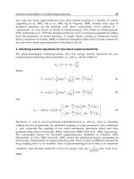
Fig. 5. Bode plot of the magnetic bearing system (a reduced 2
nd
-order model is used here)
with the designed lead compensator
5. Controller Design via Interpolation Approach
5.1 Controller Design via Interpolation Approach
A single-loop unity-feedback control system shown in Figure 3 is considered in the
controller design via the interpolation approach described in (Dorato, 1999). It was shown in
(Dorato, 1999) that any rational transfer function,
where n
p
(s) and d
p
(s) are arbitrary polynomials, can always be written as a ratio of two
coprime stable proper transfer functions,
where
and
with h(s) a Hurwitz polynomial of appropriate degree. Let U(s) be a unit in the algebra of
BIBO stable proper transfer functions, then following (Dorato, 1999) a stable stabilizing
controller can be calculated as:
when P(s) satisfies the parity-interlacing property (p.i.p.) condition (Youla, 1974) and U(s)
satisfies certain interpolation conditions. Specifically, let b
i
denotes the zeros of the plant in
the RHP, the closed-loop system will be internally stable, and the controller will be stable, if
and only if U(s) interpolates to U(b
i
) = D
p
(b
i
) (Dorato, 1999).
5.2 Controller Design for the Magnetic Bearing System
Firstly we note that the reduced order model of the plant described by equation (2) has a
zero at s =2854 and a zero at s =∞. Since the pole at s = 292.7 is not between these two zeros,
the parity-interlacing property (p.i.p.) condition (Youla, 1974) is satisfied and a stable
stabilizing controller is known to exist.
In the following, we assume that the design must satisfy the following specifications:
The sensitivity function is to have all its poles at s =-511,
A steady-state error magnitude (subjected to a unit step input) of e
ss
= 0.1.
Since the closed-loop transfer functions are:
By choosing h(s) = (s + 511)
2
, the requirement of the closed-loop poles specification will be
satisfied. As a result,
and
Magnetic Bearings, Theory and Applications8
The interpolation conditions are:
U(2854) = D
p
(2854) = 0.7612, and U(∞) = D
p
(∞) = 1.
Let the steady-state error magnitude be e
ss
= 0.1, then:
Let the interpolating unit U(s) take of the following form:
with a > 0 and b > 0, then after some simple calculations, the controller is found to be:
Controllers with other values of steady-state error magnitude can also be found by
following similar procedures. For example, the following controllers C
1
(s) and C
2
(s) were
computed on the basis of error magnitude e
ss
= 0.01 and e
ss
= 1, respectively.
It can be seen that each of these controllers is of second order and is in the form of a lead-lag
compensator.
6. Fuzzy logic controller design
A fuzzy logic controller (FLC) consists of four elements. These are a fuzzification interface, a
rule base, an inference mechanism, and a defuzzification interface (Passino & Yurkovich,
1998). A FLC has to be designed for each of the four channels of the MBC500 magnetic
system. The design of the FLC for channel x
2
is described in detail in this section. The design
of the remaining FLCs will follow the same procedure. The FLC designed for the MBC500
magnetic bearing system in this section has two inputs and one output. The “Error” and
“Rate of Change of Error” variables derived from the output from the MBC500 on-board
hall-effect sensor will be used as the inputs. A voltage for controlling the current amplifiers
on the MBC500 magnetic bearing system will be produced as the output. The shaft’s
schematic (top view) showing the electromagnets and the Hall-effect sensors is provided in
Figure 6.
Fig. 6. Shaft schematic showing electromagnets and Hall-effect sensors (Magnetic Moments,
1995)
Figure 7 shows the single channel block diagram of the magnetic bearing system with the
proposed FLC. A PD-Like FLC was designed to improve system damping as closed-loop
stability is the major concern of the magnetic bearing system. As the MBC500 is a small
magnetic bearing system, it has extremely fast dynamic responses which include the
vibrations at 770 Hz and 2050 Hz. Therefore, a sampling frequency of 20kHz (or a sample
period of 50 microseconds) was deemed necessary.
Fig. 7. FLC for MBC500 magnetic bearing system
Figure 8 illustrates the horizontal orientation (top view) of the MBC500 magnetic bearing
shaft with the corresponding centre reference line, and its output and input at the right hand
side (that is, channel 2).
Fig. 8. MBC500 magnetic bearing control at the right hand side for channel x
2
Design and implementation of conventional
and advanced controllers for magnetic bearing system stabilization 9
The interpolation conditions are:
U(2854) = D
p
(2854) = 0.7612, and U(∞) = D
p
(∞) = 1.
Let the steady-state error magnitude be e
ss
= 0.1, then:
Let the interpolating unit U(s) take of the following form:
with a > 0 and b > 0, then after some simple calculations, the controller is found to be:
Controllers with other values of steady-state error magnitude can also be found by
following similar procedures. For example, the following controllers C
1
(s) and C
2
(s) were
computed on the basis of error magnitude e
ss
= 0.01 and e
ss
= 1, respectively.
It can be seen that each of these controllers is of second order and is in the form of a lead-lag
compensator.
6. Fuzzy logic controller design
A fuzzy logic controller (FLC) consists of four elements. These are a fuzzification interface, a
rule base, an inference mechanism, and a defuzzification interface (Passino & Yurkovich,
1998). A FLC has to be designed for each of the four channels of the MBC500 magnetic
system. The design of the FLC for channel x
2
is described in detail in this section. The design
of the remaining FLCs will follow the same procedure. The FLC designed for the MBC500
magnetic bearing system in this section has two inputs and one output. The “Error” and
“Rate of Change of Error” variables derived from the output from the MBC500 on-board
hall-effect sensor will be used as the inputs. A voltage for controlling the current amplifiers
on the MBC500 magnetic bearing system will be produced as the output. The shaft’s
schematic (top view) showing the electromagnets and the Hall-effect sensors is provided in
Figure 6.
Fig. 6. Shaft schematic showing electromagnets and Hall-effect sensors (Magnetic Moments,
1995)
Figure 7 shows the single channel block diagram of the magnetic bearing system with the
proposed FLC. A PD-Like FLC was designed to improve system damping as closed-loop
stability is the major concern of the magnetic bearing system. As the MBC500 is a small
magnetic bearing system, it has extremely fast dynamic responses which include the
vibrations at 770 Hz and 2050 Hz. Therefore, a sampling frequency of 20kHz (or a sample
period of 50 microseconds) was deemed necessary.
Fig. 7. FLC for MBC500 magnetic bearing system
Figure 8 illustrates the horizontal orientation (top view) of the MBC500 magnetic bearing
shaft with the corresponding centre reference line, and its output and input at the right hand
side (that is, channel 2).
Fig. 8. MBC500 magnetic bearing control at the right hand side for channel x
2
Magnetic Bearings, Theory and Applications10
The displacement output x
2
is sensed by the Hall-effect sensor as the voltage V
sense2
. Hence
the error signal is defined for channel x
2
as:
݁
ሺ
ݐ
ሻ
ൌݎ
ሺ
ݐ
ሻ
െܸ
௦௦ଶ
ሺݐሻ
For the magnetic bearing stabilization problem, the reference input is r(t) = 0. As a result,
݁
ሺ
ݐ
ሻ
ൌെܸ
௦௦ଶ
ሺݐሻ
and
݀
݀ݐ
݁
ሺ
ݐ
ሻ
ൌെ
݀
݀ݐ
ܸ
௦௦ଶ
ሺݐሻ
The linguistic variables which describe the FLC inputs and outputs are:
“Error” denotes e(t)
“Rate of change of error” denotes
ௗ
ௗ௧
݁ሺݐሻ
“Control voltage” denotes V
control2
The above linguistic variables “error”, “rate of change of error,” and “control voltage” will
take on the following linguistic values:
“NB” = Negative Big
“NS” = Negative Small
“ZO” = Zero
“PS” = Positive Small
“PB” = Positive Big
Drawing on the design concept of the FLC for an inverted pendulum on a cart described in
(Passino & Yurkovich, 1998) the following statements can be developed to illustrate the
linguistic quantification of the different conditions of the magnetic bearing:
The statement “error is PB” represents the situation where the magnetic bearing
shaft is significantly below the reference line.
The statement “error is NS” represents the situation where the magnetic bearing
shaft is just slightly above the reference line. However, it is neither too close to the
centre reference position to be quantified as “ZO” nor it is too far away to be
quantified as “NB”.
The statement “error is ZO” represents the situation where the magnetic bearing
shaft is sufficiently close to the centre reference position. As a linguistic
quantification is not precise, any value of the error around e(t) = 0 will be accepted
as “ZO” as long as this can be considered as a better quantification than “PS” or
”NS”.
The statement “error is PB and rate of change of error is PS” represents the
situation where the magnetic bearing shaft is significantly below the centre
reference line and, since
ௗ
ௗ௧
ܸ
௦௦ଶ
൏Ͳ, the magnetic bearing shaft is moving slowly
away from the centre position.
The statement “error is NS and rate of change of error is PS” represents the
situation where the magnetic bearing shaft is slightly above the centre reference
line and, since
ௗ
ௗ௧
ܸ
௦௦ଶ
൏Ͳ, the magnetic bearing shaft is moving slowly towards
the centre position.
We shall use the above linguistic quantification to specify a set of rules or a rule-base. The
following three situations will demonstrate how the rule-base is developed.
1. If error is NB and rate of change of error is NB Then force is NB.
Figure 9 shows that the magnetic bearing shaft at the right end is significantly above the
centre reference line and is moving away from it quickly. Therefore, it is clear that a strong
negative force should be applied so that the shaft will move to the centre reference position.
Fig. 9. Magnetic bearing shaft at the right end with a positive displacement
2. If error is ZO and rate of change of error is PS Then force is PS.
Figure 10 shows that the bearing shaft at the right end has a displacement of nearly zero
from the centre reference position (a linguistic quantification of zero does not imply that
e(t)=0 exactly) and is moving away (downwards) from the centre reference line. Therefore, a
small positive force should be applied to counteract the movement so that it will move
towards the centre reference position.
Fig. 10. Magnetic bearing shaft at the right end with zero displacement
3. If error is PB and rate of change of error is NS Then force is PS.
Figure 11 shows that the bearing shaft at the right end is far below the centre reference line
and is moving towards the centre reference position. Therefore, a small positive force should
be applied to assist the movement. However, it should not be too large a force since the
bearing shaft at the right end is already moving in the correct direction.
Design and implementation of conventional
and advanced controllers for magnetic bearing system stabilization 11
The displacement output x
2
is sensed by the Hall-effect sensor as the voltage V
sense2
. Hence
the error signal is defined for channel x
2
as:
݁
ሺ
ݐ
ሻ
ൌݎ
ሺ
ݐ
ሻ
െܸ
௦௦ଶ
ሺݐሻ
For the magnetic bearing stabilization problem, the reference input is r(t) = 0. As a result,
݁
ሺ
ݐ
ሻ
ൌെܸ
௦௦ଶ
ሺݐሻ
and
݀
݀ݐ
݁
ሺ
ݐ
ሻ
ൌെ
݀
݀ݐ
ܸ
௦௦ଶ
ሺݐሻ
The linguistic variables which describe the FLC inputs and outputs are:
“Error” denotes e(t)
“Rate of change of error” denotes
ௗ
ௗ௧
݁ሺݐሻ
“Control voltage” denotes V
control2
The above linguistic variables “error”, “rate of change of error,” and “control voltage” will
take on the following linguistic values:
“NB” = Negative Big
“NS” = Negative Small
“ZO” = Zero
“PS” = Positive Small
“PB” = Positive Big
Drawing on the design concept of the FLC for an inverted pendulum on a cart described in
(Passino & Yurkovich, 1998) the following statements can be developed to illustrate the
linguistic quantification of the different conditions of the magnetic bearing:
The statement “error is PB” represents the situation where the magnetic bearing
shaft is significantly below the reference line.
The statement “error is NS” represents the situation where the magnetic bearing
shaft is just slightly above the reference line. However, it is neither too close to the
centre reference position to be quantified as “ZO” nor it is too far away to be
quantified as “NB”.
The statement “error is ZO” represents the situation where the magnetic bearing
shaft is sufficiently close to the centre reference position. As a linguistic
quantification is not precise, any value of the error around e(t) = 0 will be accepted
as “ZO” as long as this can be considered as a better quantification than “PS” or
”NS”.
The statement “error is PB and rate of change of error is PS” represents the
situation where the magnetic bearing shaft is significantly below the centre
reference line and, since
ௗ
ௗ௧
ܸ
௦௦ଶ
൏Ͳ, the magnetic bearing shaft is moving slowly
away from the centre position.
The statement “error is NS and rate of change of error is PS” represents the
situation where the magnetic bearing shaft is slightly above the centre reference
line and, since
ௗ
ௗ௧
ܸ
௦௦ଶ
൏Ͳ, the magnetic bearing shaft is moving slowly towards
the centre position.
We shall use the above linguistic quantification to specify a set of rules or a rule-base. The
following three situations will demonstrate how the rule-base is developed.
1. If error is NB and rate of change of error is NB Then force is NB.
Figure 9 shows that the magnetic bearing shaft at the right end is significantly above the
centre reference line and is moving away from it quickly. Therefore, it is clear that a strong
negative force should be applied so that the shaft will move to the centre reference position.
Fig. 9. Magnetic bearing shaft at the right end with a positive displacement
2. If error is ZO and rate of change of error is PS Then force is PS.
Figure 10 shows that the bearing shaft at the right end has a displacement of nearly zero
from the centre reference position (a linguistic quantification of zero does not imply that
e(t)=0 exactly) and is moving away (downwards) from the centre reference line. Therefore, a
small positive force should be applied to counteract the movement so that it will move
towards the centre reference position.
Fig. 10. Magnetic bearing shaft at the right end with zero displacement
3. If error is PB and rate of change of error is NS Then force is PS.
Figure 11 shows that the bearing shaft at the right end is far below the centre reference line
and is moving towards the centre reference position. Therefore, a small positive force should
be applied to assist the movement. However, it should not be too large a force since the
bearing shaft at the right end is already moving in the correct direction.
Magnetic Bearings, Theory and Applications12
Fig. 11. Magnetic bearing shaft at the right end with a negative displacement
Following a similar analysis, the rules of the FLC for controlling the magnetic bearing shaft
can be developed. For the FLC with two inputs and five linguistic values for each input,
there are 5
2
=25 possible rules with all combination for the inputs. A set of possible linguistic
output values are NB, NS, ZO, PS and PB. The tabular representation of the FLC rule base
(with 25 rules) of the magnetic bearing fuzzy control system is shown in Table 1.
“control voltage”
“rate of change of error”݁
ሶ
V NB NS ZO PS PB
“error”e
NB NB NB NB NS ZO
NS NB NB NS ZO PS
ZO NB NS ZO PS PM
PS NS ZO PS PB PB
PB ZO PS PB PB PB
Table 1. Rule table with 25 rules
The membership functions to be employed are of the triangular type where, for any given
input, there are only two membership functions premises to be calculated. This is in contrast
to Gaussian membership functions where each requires more than two premise outputs and
can generate a large amount of calculations per final output. The triangular membership
functions used is shown in Figure 12:
Fig. 12. Triangular Membership Function
-1.5 -1 -0.5 0 0.5 1 1.5
0
0.2
0.4
0.6
0.8
1
System Input
Membership Function Output
The membership functions shown in Figure 12 represent the linguistic values NB, NS, ZO,
PS, PB (from left to right).
The inference method used for the designed FLC is Takagi-Sugeno Method (Passino &
Yurkovich, 1998) and the centre average method is used in the defuzzification process
(Passino & Yurkovich, 1998).
7. Simulation Results
By using the designed conventional controller C
lead
(s), the controllers C(s), C
1
(s), and C
2
(s)
designed via the analytical interpolation method, and the FLC designed in Section 6, the
closed-loop responses to a unit-step reference (applied at t = 0) and a unit-step disturbance
(applied at t = 0.05 seconds) and the corresponding control signals are shown in Figure 13
and Figure 14, respectively. In all of the simulations, the full 8
th
-order plant model described
by equation (1) was employed.
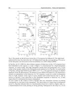
It is important to note that the DC gain designed into each of C(s) and C
1
(s) via interpolation
has forced the steady-state error to be the small value specified. It is also important to note
that while the closed-loop unit step responses with C
lead
(s) and C
2
(s) have comparable
steady-state errors (approximately -1), the closed-loop unit-step response with C
2
(s) has a
much better transient responses than that with C
lead
(s). (Similar comment also applies to their
disturbance rejection behaviours). Furthermore, it is apparent that trade-off between steady-
state error and transient response can be easily achieved with controllers designed via the
interpolation approach presented in Section 5.
Fig. 13. Closed-loop responses of the MBC500 magnetic bearing system to step reference and
step disturbance with controllers C
lead
(s), C(s), C
1
(s), and C
2
(s), and the designed FLC.
Design and implementation of conventional
and advanced controllers for magnetic bearing system stabilization 13
Fig. 11. Magnetic bearing shaft at the right end with a negative displacement
Following a similar analysis, the rules of the FLC for controlling the magnetic bearing shaft
can be developed. For the FLC with two inputs and five linguistic values for each input,
there are 5
2
=25 possible rules with all combination for the inputs. A set of possible linguistic
output values are NB, NS, ZO, PS and PB. The tabular representation of the FLC rule base
(with 25 rules) of the magnetic bearing fuzzy control system is shown in Table 1.
“control voltage”
“rate of change of error”݁
ሶ
V NB NS ZO PS PB
“error”e
NB NB NB NB NS ZO
NS NB NB NS ZO PS
ZO NB NS ZO PS PM
PS NS ZO PS PB PB
PB ZO PS PB PB PB
Table 1. Rule table with 25 rules
The membership functions to be employed are of the triangular type where, for any given
input, there are only two membership functions premises to be calculated. This is in contrast
to Gaussian membership functions where each requires more than two premise outputs and
can generate a large amount of calculations per final output. The triangular membership
functions used is shown in Figure 12:
Fig. 12. Triangular Membership Function
-1.5 -1 -0.5 0 0.5 1 1.5
0
0.2
0.4
0.6
0.8
1
System Input
Membership Function Output
The membership functions shown in Figure 12 represent the linguistic values NB, NS, ZO,
PS, PB (from left to right).
The inference method used for the designed FLC is Takagi-Sugeno Method (Passino &
Yurkovich, 1998) and the centre average method is used in the defuzzification process
(Passino & Yurkovich, 1998).
7. Simulation Results
By using the designed conventional controller C
lead
(s), the controllers C(s), C
1
(s), and C
2
(s)
designed via the analytical interpolation method, and the FLC designed in Section 6, the
closed-loop responses to a unit-step reference (applied at t = 0) and a unit-step disturbance
(applied at t = 0.05 seconds) and the corresponding control signals are shown in Figure 13
and Figure 14, respectively. In all of the simulations, the full 8
th
-order plant model described
by equation (1) was employed.
It is important to note that the DC gain designed into each of C(s) and C
1
(s) via interpolation
has forced the steady-state error to be the small value specified. It is also important to note
that while the closed-loop unit step responses with C
lead
(s) and C
2
(s) have comparable
steady-state errors (approximately -1), the closed-loop unit-step response with C
2
(s) has a
much better transient responses than that with C
lead
(s). (Similar comment also applies to their
disturbance rejection behaviours). Furthermore, it is apparent that trade-off between steady-
state error and transient response can be easily achieved with controllers designed via the
interpolation approach presented in Section 5.
Fig. 13. Closed-loop responses of the MBC500 magnetic bearing system to step reference and
step disturbance with controllers C
lead
(s), C(s), C
1
(s), and C
2
(s), and the designed FLC.
Magnetic Bearings, Theory and Applications14
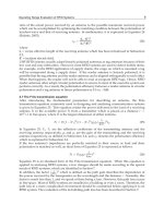
Fig. 14. Closed-loop responses of the MBC500 magnetic bearing system to step reference and
step disturbance with controllers C
lead
(s), C(s), C
1
(s), and C
2
(s), and the designed FLC.
It can also be observed that the closed-loop unit step responses obtained with the designed
FLC exhibits more oscillations. However, it must be pointed out that two elliptic notch
filters to notch out the resonant modes of the MBC500 magnetic bearing system located at
approximately 770 Hz and 2050 Hz were employed with both the conventional controller
and the controllers designed via analytical interpolation approach to ensure system stability.
For the designed FLC, system stability is achieved without the need of using the two notch
filters.
From Figures 13 and 14 it can be seen that the system is stable and reasonably well
compensated by all the controllers designed. These controllers are now ready to be coded in
C language and implemented in real-time.
8. Implementation of the designed Controllers
In order to implement the designed notch filters and controllers, a dSPACE DS1102
processor board, MatLab, Simulink and dSPACE Control Desk are used. The controllers
C
lead
(s) and C
2
(s) are represented as a block diagram via a Simulink file, which allows it to be
connected to the ADC and the DAC of the DS1102 processor board. The DS1102 DSP board
can then execute the designed controllers (discretized via the bilinear-transformation
method) through MatLab’s Real-Time Workshop.
In this magnetic bearing system, for the model based controllers the notch filters act to
provide damping to the rotor resonances near 770 Hz and 2050 Hz. The sampling frequency
was originally chosen to be 25 kHz to avoid aliasing of frequencies within the normal
operating frequency range (Shi & Revell, 2002). The maximum possible sampling frequency
with the FLC was 20 kHz (Shi & Lee, 2008) due to the longer C code implementation
requirement of the FLC. In order to have a fair comparison of the system responses, the
sampling frequencies of the model based controllers and the FLC were both set at 20kHz.
In the following, we shall present and compare the experimental results. Preliminary
observation has revealed that the performance of the controller C
2
(s) designed via analytical
interpolation approach is most similar to C
lead
(s) and the FLC. As a result, the performance of
C
2
(s) will be investigated in detail in the implementation. We shall first compare the results
for the model based controllers and the FLC under steady-state conditions. We shall then
compare the disturbance rejection results of the closed-loop system employing each of these
controllers.
8.1 Comparison of Steady-state Responses
Figure 15 shows the steady-state responses of the magnetic bearing system when it is under
the control of the model based controllers and the FLC, respectively.
Fig. 15. Steady-state responses with the model based controllers and FLC
It can be seen in Figure 15 that the displacement sensor outputs were noisy when the
magnetic bearing system is controlled by either the model based controller or the FLC.
However, the response with the FLC has a smaller steady-state error (i.e. closer to zero).
Investigation via analysis and simulation has revealed that the source of the noise in the
outputs was measurement noise.
Design and implementation of conventional
and advanced controllers for magnetic bearing system stabilization 15
Fig. 14. Closed-loop responses of the MBC500 magnetic bearing system to step reference and
step disturbance with controllers C
lead
(s), C(s), C
1
(s), and C
2
(s), and the designed FLC.
It can also be observed that the closed-loop unit step responses obtained with the designed
FLC exhibits more oscillations. However, it must be pointed out that two elliptic notch
filters to notch out the resonant modes of the MBC500 magnetic bearing system located at
approximately 770 Hz and 2050 Hz were employed with both the conventional controller
and the controllers designed via analytical interpolation approach to ensure system stability.
For the designed FLC, system stability is achieved without the need of using the two notch
filters.
From Figures 13 and 14 it can be seen that the system is stable and reasonably well
compensated by all the controllers designed. These controllers are now ready to be coded in
C language and implemented in real-time.
8. Implementation of the designed Controllers
In order to implement the designed notch filters and controllers, a dSPACE DS1102
processor board, MatLab, Simulink and dSPACE Control Desk are used. The controllers
C
lead
(s) and C
2
(s) are represented as a block diagram via a Simulink file, which allows it to be
connected to the ADC and the DAC of the DS1102 processor board. The DS1102 DSP board
can then execute the designed controllers (discretized via the bilinear-transformation
method) through MatLab’s Real-Time Workshop.
In this magnetic bearing system, for the model based controllers the notch filters act to
provide damping to the rotor resonances near 770 Hz and 2050 Hz. The sampling frequency
was originally chosen to be 25 kHz to avoid aliasing of frequencies within the normal
operating frequency range (Shi & Revell, 2002). The maximum possible sampling frequency
with the FLC was 20 kHz (Shi & Lee, 2008) due to the longer C code implementation
requirement of the FLC. In order to have a fair comparison of the system responses, the
sampling frequencies of the model based controllers and the FLC were both set at 20kHz.
In the following, we shall present and compare the experimental results. Preliminary
observation has revealed that the performance of the controller C
2
(s) designed via analytical
interpolation approach is most similar to C
lead
(s) and the FLC. As a result, the performance of
C
2
(s) will be investigated in detail in the implementation. We shall first compare the results
for the model based controllers and the FLC under steady-state conditions. We shall then
compare the disturbance rejection results of the closed-loop system employing each of these
controllers.
8.1 Comparison of Steady-state Responses
Figure 15 shows the steady-state responses of the magnetic bearing system when it is under
the control of the model based controllers and the FLC, respectively.
Fig. 15. Steady-state responses with the model based controllers and FLC
It can be seen in Figure 15 that the displacement sensor outputs were noisy when the
magnetic bearing system is controlled by either the model based controller or the FLC.
However, the response with the FLC has a smaller steady-state error (i.e. closer to zero).
Investigation via analysis and simulation has revealed that the source of the noise in the
outputs was measurement noise.
Magnetic Bearings, Theory and Applications16
8.2 Comparison of Step and Disturbance Rejection Responses
Figure 16 and Figure 17 show the displacement sensor output and the controller output,
respectively, when a step disturbance of 0.05V is applied to the channel 1 input of the
magnetic bearing system when it is controlled with the model based conventional controller
C
lead
(s). Note that the displacement sensor output is multiplied by a factor of 10 when it is
transmitted through the DAC.
Fig. 16. Displacement output of the MBC500 magnetic bearing system with the model based
controller C
lead
(s).
Fig. 17. Control signal of the MBC500 magnetic bearing system with the model based
controller C
lead
(s).
Figure 18 and Figure 19 show the displacement sensor output and the controller output,
respectively, when a step change in disturbance of 0.1V is applied to the channel 1 input of
the magnetic bearing system when it is controlled with the model based controller.
Fig. 18. Step response of the MBC500 magnetic bearing system with the model based
controller C
lead
(s).
Fig. 19. Control signal of the MBC500 magnetic bearing system with the model based
controller C
lead
(s).
Design and implementation of conventional
and advanced controllers for magnetic bearing system stabilization 17
8.2 Comparison of Step and Disturbance Rejection Responses
Figure 16 and Figure 17 show the displacement sensor output and the controller output,
respectively, when a step disturbance of 0.05V is applied to the channel 1 input of the
magnetic bearing system when it is controlled with the model based conventional controller
C
lead
(s). Note that the displacement sensor output is multiplied by a factor of 10 when it is
transmitted through the DAC.
Fig. 16. Displacement output of the MBC500 magnetic bearing system with the model based
controller C
lead
(s).
Fig. 17. Control signal of the MBC500 magnetic bearing system with the model based
controller C
lead
(s).
Figure 18 and Figure 19 show the displacement sensor output and the controller output,
respectively, when a step change in disturbance of 0.1V is applied to the channel 1 input of
the magnetic bearing system when it is controlled with the model based controller.
Fig. 18. Step response of the MBC500 magnetic bearing system with the model based
controller C
lead
(s).
Fig. 19. Control signal of the MBC500 magnetic bearing system with the model based
controller C
lead
(s).
Magnetic Bearings, Theory and Applications18
Figure 20 and Figure 21 show the displacement sensor output and the controller output,
respectively, when a step change in disturbance of 0.5V is applied to the channel 1 input of
the magnetic bearing system when it is controlled with the conventional controller C
lead
(s).
Fig. 20. Step response of the MBC500 magnetic bearing system with the model based
controller C
lead
(s).
Fig. 21. Control signal of the MBC500 magnetic bearing system with the model based
controller C
lead
(s).
It can be seen from the above figures that the magnetic bearing system remain stable under
the control of the model based conventional controller when a step change in disturbance of
is applied to its channel 1 input. Similar results were also obtained from other channels.
Figure 22 and Figure 23 show the displacement sensor output and the controller output,
respectively, when a step change in disturbance of 0.05V is applied to the channel 1 input of
the magnetic bearing system when it is controlled with the analytical controller C
2
(s).
Fig. 22. Displacement output of the MBC500 magnetic bearing system with the analytical
controller C
2
(s).
Fig. 23. Control signal of the MBC500 magnetic bearing system with the analytical controller
C
2
(s).
Design and implementation of conventional
and advanced controllers for magnetic bearing system stabilization 19
Figure 20 and Figure 21 show the displacement sensor output and the controller output,
respectively, when a step change in disturbance of 0.5V is applied to the channel 1 input of
the magnetic bearing system when it is controlled with the conventional controller C
lead
(s).
Fig. 20. Step response of the MBC500 magnetic bearing system with the model based
controller C
lead
(s).
Fig. 21. Control signal of the MBC500 magnetic bearing system with the model based
controller C
lead
(s).
It can be seen from the above figures that the magnetic bearing system remain stable under
the control of the model based conventional controller when a step change in disturbance of
is applied to its channel 1 input. Similar results were also obtained from other channels.
Figure 22 and Figure 23 show the displacement sensor output and the controller output,
respectively, when a step change in disturbance of 0.05V is applied to the channel 1 input of
the magnetic bearing system when it is controlled with the analytical controller C
2
(s).
Fig. 22. Displacement output of the MBC500 magnetic bearing system with the analytical
controller C
2
(s).
Fig. 23. Control signal of the MBC500 magnetic bearing system with the analytical controller
C
2
(s).
Magnetic Bearings, Theory and Applications20
Figure 24 and Figure 25 show the displacement sensor output and the controller output,
respectively, when a step change in disturbance of 0.1V is applied to the channel 1 input of
the magnetic bearing system when it is controlled with the analytical controller C
2
(s).
Fig. 24. Displacement output of the MBC500 magnetic bearing system with the analytical
controller C
2
(s).
Fig. 25. Control signal of the MBC500 magnetic bearing system with the analytical controller
C
2
(s).
Figure 26 and Figure 27 show the displacement sensor output and the controller output,
respectively, when a step change in disturbance of 0.5V is applied to the channel 1 input of
the magnetic bearing system when it is controlled with the analytical controller C
2
(s).
Fig. 26. Displacement output of the MBC500 magnetic bearing system with the analytical
controller C
2
(s).
Fig. 27. Control signal of the MBC500 magnetic bearing system with the analytical controller
C
2
(s).