Self Organizing Maps Applications and Novel Algorithm Design Part 7 doc
Bạn đang xem bản rút gọn của tài liệu. Xem và tải ngay bản đầy đủ của tài liệu tại đây (1.05 MB, 40 trang )
Self Organizing Maps - Applications and Novel Algorithm Design
230
comprehensible because ship No. 5 is the oldest version of this vessel. Next the new group
was created, which was separated from the area activated before by ship No. 5. The new
map of partition for area of activation looks like is presented on figure 15.
Ship no.
Data
1 2 3 4 5
presented before 94.5% 96.0% 92.3% 95.3% 92.8%
not presented
before
72.1% 69.4% 75.8% 73.5% 77.2%
Table 3. The number of correct classifications
Fig. 15. The new map of partition for area of activation for researched ships after
introducing new ship
6. Conclusion
As it is shown on results the used Self-Organizing Map is useful for ships classification
based on its hydroacoustics signature. Classification of signals that were used during
learning process, characterize the high number of correct answer (above 90%) what was
expected. This result means that used Kohonen network associated with feedforward
network has been correctly configured and learned. Presentation of signals that weren’t
used during learning process, gives lowest value of percent of correct answer than in
previous case but this results is very high too (about 70 % of correct classification). This
means that neural classifier has good ability to generalize the knowledge. More over after
Ship’s Hydroacoustics Signatures Classification Using Neural Networks
231
presentation of new ship which weren’t taking into account during creating classifier, the
Kohonen networks was able to create new group dividing the group which belongs to the
similar type of ship. After few cycles used neural networks expand its output vector or in
other words map of membership about new area of activation. This means that used
Kohonen networks has possibility to develop its own knowledge so it cause that
presented method of classification is very flexible and is able to adaptation to changing
conditions.
Presented case is quite simple because it not take into account that object sounds change
with time, efficiency conditions (e.g. some elements of machinery are damaged), sound
rates, etc. It doesn’t consider the influence of changes of environment on acquired
hydroacoustics signals. In next step of research the proper work of this method will be
checked for enlarged vector of objects. The hydroacoustics signatures of ships were
acquired in different environmental conditions and in different stage of ship operating.
Therefore the cases of changing hydroacoustics signatures which were mentioned before
should be investigated too.
In future research the influence of network configuration on the quality of classification
should be checked. More over some consideration about feature extracting from
hydroacoustics signature should be made.
Described method after successful research mentioned above and after preparation for
work in real time will be extended and its application is provided as assistant subsystem
for passive hydrolocations systems of Polish Naval ships.
The aim of presented method is to classify and recognize ships basing on its acoustic
signatures. This method can found application in intelligence submarine weapon and in
hydrolocation systems. In other hand it is important to deform and cheat the similar
system of our opponents by changing the “acoustic portrait” of own ships. From the point
of ship’s passive defense view it is desirable to minimize the range of acoustic signatures
propagation. Noise isolation systems for vessels employ a wide range of techniques,
especially double-elastic devices in the case of diesel generators and main engines. Also,
rotating machinery and moving parts should be dynamically-balanced to reduce the
noise. In addition, the equipment should be mounted in special acoustically insulated
housings (special kind of containers). One of the method to change the hydroacoustics
signatures is to pump the air under the hull of ship. It cause the offset of generated by
moving ship frequency into the direction of high frequency, the same the range of
propagation become smaller.
7. References
Fort J. C., SOM’s mathematics, Neural Networks, 19: 812–816, 2006
Gloza I., Malinowski S. J., Underwater Noise Radaited by Ships, Their Propulsion and
Auxiliary Machinery and Propellers, Hydroacoustics vol. 4, pp. 165-168, 2001
Gloza I., Malinowski S. J., Underwater Noise Characteristics of Small Ships, Acta Acoustica
United with Acustica, vol. 88 pp. 718-721, 2002
Haykin S., Self-organizing maps, Neural networks - A comprehensive foundation, 2nd edition,
Prentice-Hall, 1999
Kohonen T., Self-Organizing Maps, Third, extended edition, Springer, 2001
Osowski S., Neural Networks, Publishing House of Warsaw University of Technology, 1996
Stąpor K., Automatic object classification, Publishing House EXIT 2005
Self Organizing Maps - Applications and Novel Algorithm Design
232
Szczepaniak P. S., Intelligence Calculations, Fast Transforms and Classification, Publishing
House EXIT, 2004
Therrien Ch. W., Discrete Random Signals and Statistical Signal Processing, Prentice Hall
International, Inc. 1992
Urick R. J., Principles of Underwater Sounds, McGraw-Hill, New York 1975
Zak A., Creating patterns for hydroacoustics signals, Hydroacoustics Vol. 8, pp. 265- 270, 2005
Zak A., Neural Classification Of Ships Hydroacoustics Signatures, Proceedings of the 9th
European Conference on Underwater Acoustics ECUA 2008, Paris, France 2008, pp.
829-834
13
Dynamic Vehicle Routing Problem for
Medical Emergency Management
Jean-Charles Créput
1
, Amir Hajjam
1
,
Abderrafiãa Koukam
1
and Olivier Kuhn
2,3
1
Systems and Transportation Laboratory, U.T.B.M., 90010 Belfort Cedex,
2
Université Lyon 1, LIRIS, UMR5205, F-69622 Villeurbanne,
3
Université de Lyon, CNRS
France
1. Introduction
Nowadays telemedicine applications are more and more present in the state-of-the-art
medicine. Telemedicine is a good way to improve access to healthcare, quality of care,
reduce isolation and also costs. In that way we can now safely perform surgery between two
places separated by several thousand km, navigate in 3D models of blood vessels or
generate 3D models from Nuclear-Magnetic Resonance Imaging (MRI). But there is
currently a lack of tools for all day medical acts which could improve medical system
efficiency especially for medical emergency services.
In order to help medical emergency services, the project MERCURE (Mobile and Network
for the Private clinic, the Urgency or the External Residence) has been launched in order to
create tools that optimize, follow and manage emergency interventions. The current
problem is that the choice of the doctor for a patient is done by hand.The call center is
neither aware of the exact location nor the current state of the doctors. Thus it is rarely the
best located doctor who is chosen and moreover he may not have correct equipments to heal
the patient. To optimize that aspect, we have developed software allowing the optimized
management of human and material medical resources.
This problem, conventionally called vehicle routing problem (VRP), is one of the most
widely studied problems in combinatorial optimization. In the standard VRP, a fleet of
vehicles must be routed to visit a set of customers at minimum cost, subject to vehicle
capacity constraint and route duration constraint. In the static version of the problem, it is
assumed that all customers are known in advance to the planning process. In the case of
medical emergency management, it includes some dynamic elements. The information data
often tends to be uncertain or even unknown at the time of the planning. It may be the case
that patients, driving times or service times, are unknown before the day of operation has
begun, but become available in real-time. Due to the recent advances in information and
communication technologies, such as geographic information systems (GIS), global
positioning systems (GPS) and mobile phones, companies are now able to manage vehicle
routes in real-time. Hence, with the increased access to these services, the need for robust
real-time optimization procedures will be of critical importance, for small to big distribution
companies, whose logistics are based on a high reactivity to the customer demand.
Self Organizing Maps - Applications and Novel Algorithm Design
234
As for static vehicle routing problems, a lot of versions of the dynamic problem exist
depending on application areas. For an overview and classification of the numerous
versions of real-time routing and dispatching problems, we refer the reader to the general
surveys and classifications given in (Ghiani & al., 2003), (Larsen, 2000), (Larsen &al., 2008),
(Gendreau &Potvin, 1998) and (Psaraftis, 1995), (Psaraftis, 1998). One of the simplest
versions is the standard dynamic VRP with capacity and time duration constraints (Kilby &
al., 1998), called “dynamic VRP” in this paper, which is a straightforward extension of the
classical static VRP (Christofides & al., 1979). In this problem, the customers are the only
elements which have a dependence on time. Customers are not known in advance but arrive
as the day progresse. The system has to incorporate them into the already designed routes in
real time. Problems fitting this model appear frequently in industry.
A lot of different versions of the dynamic VRP have been studied, whereas very few
dynamic routing problems except the dynamic VRPTW or dynamic PDPTW are recognized
as standard problems well suited to allow comparative evaluations of heuristics and
metaheuristics on a common set of benchmarks. For example, only two papers on the
dynamic VRP that shared detailed results on a common test set have been found. They are
first an adaptation of the ant colony approach MACS-VRPTW Gambardella & al., 1999) by
(Montemanni & al., 2005), and second a genetic algorithm (Goncalves & al., 2007). They
share results (Kilby & al., 1998), test set with 22 problems of sizes from 50 with up to 385
customers. This paper tries to go one step further in that direction considering the dynamic
VRP as a standard dynamic problem, and yielding a comparative study with these two
methods on the Kilby et al. test set. Then, we restrict the scope of our work to the dynamic
VRP, with capacity and time duration constraints.
In the following section, the MERCURE project will be presented. In section 3 we shall
introduce our optimization system with implementation details. Then, section 4 reports
experiments carried out on the Kilby at al. benchmark and the comparisons made with a
state-of-the-art ant colony approach and a genetic algorithm already studied on these
benchmarks. Finally, last section is devoted to the conclusion and further research.
2. Project MERCURE
2.1 Aim of the project
The project MERCURE takes part in the French pole of competitiveness therapeutic
innovations. The aim of the project is to give, thanks to information technologies, an
optimized and dynamic management of resources used in the scope of urgentist
interventions like material and human resources. The system gives a real-time tracking of
current interventions, from the reception of the call to the closure of the medical record. It
optimizes resources, travel times and takes care of whole constraints relative to the domain:
emergency level, pathology, medical competences, location and other specific aspects
related to this profession.
The platform exploits satellite location system associated with a geographical information
system (GIS) and is based on results coming from works on vehicle routing problems
(Creput & al., 2007). With present technologies we can have accurate current location of
patients and doctors via GIS and A-GPS1 respectively. The A-GPS system has 3 main uses.
1. Know the position of each medical team.
2. Help the doctor to reach quickly the intervention point.
3. Track in real-time medical teams and resources.
Dynamic Vehicle Routing Problem for Medical Emergency Management
235
Fig. 1. Data exchanges after a patient call
Here is a basic scenario when an emergency call arrives (see figure 1). Call center point of
view:
• Information about the patient (name, address, pathology…) is inputted in the software.
• Patient’s information are processed, a set of doctors which suit to the patient’s needs is
created (depending of the pathology, the intervention area…).
• The selection of a doctor in the previously created set is done via an optimization
algorithm. Here we focus on optimizing several criteria like distance, reaction time. . .
The patient is inserted in the doctor’s road.
• The selected doctor is warned by a message on his PDA2.
Now from a doctor point of view:
• The doctor receives a patient request on his PDA and he is geo-guided to the patient’s
location via A-GPS.
• As soon as he arrives, all information about the patient are shown: previous diseases,
his allergy, current treatments. . . Those information are transferred from the database
via radio link like GPRS3 or UMTS4 for example.
• When the auscultation is finished, he inputs results and notes that are immediately
transferred to the central database. Then he goes on with the next patient.
2.2 Improvements
This whole process improves reaction time of emergency services and thus save lives. It also
provides an unique database gathering up-to-date information about patients and so
facilitate the follow-up of patients. Another main improvement is that the answer fits to the
Self Organizing Maps - Applications and Novel Algorithm Design
236
patient’s needs. In other words, the call is answered by a doctor-regulator who is able to
help the patient to describe and specify his illness. This is a real telemedicine act and thus
the software is able to select the appropriate doctor or send an ambulance. Moreover this
system may suit to other emergency services like fire brigade or police department with
some adaptations. There are some papers about ambulances location and relocation models
written by (Gendreau & al., 1997), (Gendreau & al., 1999), (Gendreau & al., 2001) and
(Brotcorne & al., 2003). But currently we are not aware of other tools for such size of
emergency services. This project is realizable thanks to recent new technologies like A-GPS,
wireless data communication and improvements in artificial intelligence and operations
research for dynamic problems.
3. Dynamic optimization system for urgentist
In the MERCURE project, we are in charge of the optimization part for the selection of
doctors and assignment of patients. We have tackled this problem as an operations research
problem named Vehicle Routing Problem (VRP) (Toth & Vigo, 2001).
3.1 Problem statement
Allan Larsen stated in his PhD report (Larsen, 2000) that emergency services have 2 major
criteria (see figure 2):
- They are highly dynamic: most or all requests are unknown at the beginning and we
have no information about their arrival time.
- The response time must be very low because lives can be in danger.
Fig. 2. Framework for classifying dynamic routing problems by their degree of dynamism
and their objective
Dynamic Vehicle Routing Problem for Medical Emergency Management
237
That is why we have chosen to represent the emergency problem as a Dynamic Vehicle
Routing Problem with Time Window (DVRPTW) which is presented in the next paragraph.
This extension of the well known VRP suits very well to this kind of problem because it takes
care of the 2 criteria previously stated. Time windows are perfect to consider response time
and the dynamic aspect allows the system to receive requests during the optimization process.
1) DVRPTW presentation: A Dynamic Vehicle Routing Problem with Time Windows is a
specialization of the well known Vehicle Routing Problem. The static VRP is defined on a set
V = {v
0
, v
1
, , v
N
} of vertices, where vertex v
0
is a depot at which are based m identical
vehicles of capacity Q, while the remaining N vertices represent customers, also called
requests, orders or demands. A non-negative cost, or travel time, is defined for each edge (v
i
,
v
j
) ∈ V × V. Each customer has a non-negative load q(v
i
) and a non-negative service time
s(v
i
). A vehicle route is a circuit on vertices. The VRP consists of designing a set of m vehicle
routes of least total cost, each starting and ending at the depot, such that each customer is
visited exactly once by a vehicle, the total demand of any route does not exceed Q, and the
total duration of any route does not exceed a preset bound T (see figure 3).
Fig. 3. Example of dynamic vehicle routing problem with 7 static requests and 2 immediate
requests
As it is the mostly done in practice (Cordeau & al., 2005), we address the Euclidean VRP
where each vertex v
i
has a location in the plane, and where the travel cost is given by the
Euclidean distance d(v
i
, v
j
) for each edge (v
i
, v
j
) ∈ V × V. Then, the objective for the static
problem is the total route length (Length) defined by
()
()
()
i
i
ii i i
jj k
i mj k
Length d , d , d ,
101 0
1, , 1, , 1
νν νν ν ν
+
==−
⎛⎞
=++
⎜⎟
⎜⎟
⎝⎠
∑∑
(1)
where
i
j
ν
∈V, 0 ≤ j ≤ k
i
, 0 ≤ k
i
≤ N, are the ordered set of demands served by the vehicle i, 1 ≤ i
≤ m, i.e. the vehicle route. The capacity constraint is defined by
(
)
i
i
j
jk
1, ,
ν
=
≤
∑
,
{
}
im1, ,∈ (2)
Self Organizing Maps - Applications and Novel Algorithm Design
238
then, assuming without loss of generality that the vehicle speed has value 1 the time
duration constraint is given by
(
)
(
)
(
)
(
)
i
ii
iiiii
jjj k
jk jk
sd,d,d,T
101 0
1, , 1, , 1
ννννννν
+
==−
+
++≤
∑∑
,
{
}
im1, ,∈
(3)
The problem is NP-hard. Thus, using heuristics is encouraged in that they have statistical or
empirical guaranty to find good solutions for large scale problems with several hundreds of
customers. For example, the most powerful Operations Research (OR) heuristics for the VRP,
referred in the extensive surveys (Gendreau & al., 2002), (Cordeau & al., 2005), are based on
metaheuristic frameworks as the Tabu Search, simulated annealing, and population based
methods, such as evolutionary algorithms, adaptive memory and ant algorithms. Other
methods can hybridize several metaheuristics principles, such as for example the very
powerful active guided local search (Mester & Bräysy, 2005), which is maybe the overall
winner approach considering both quality solution and computation time.
In the static VRP, vehicles must be routed to visit a set of customers at minimum cost,
assuming that all orders for all customers are known in advance. However, in the dynamic
VRP, new tasks enter the system and must be incorporated into the vehicle schedules and
served as the day progresses. In real-time distribution systems, demands arrive randomly in
time and the dispatching of vehicles is a continuous process of collecting demands, forming
and optimizing tours, and dispatching requests to vehicles in order to process requests at the
required geographic locations. In the case of the static VRP, the three phases of demands
reception, routes optimization and vehicles travelling are clearly separated and sequentially
performed, the output of a given phase being the input of the subsequent one. At the opposite,
we can see the dynamic VRP as an extension of the static VRP where these three time-
dependent processes are merged into an approximately same period of time. This period of
time is called the working day or planning horizon of length D. Here, we precisely define the
working day length D as the length of the collecting period, knowing that the optimization
period and the vehicle travelling period would have to be of approximately the same length.
It is often the case that in real life situations the objective function consists of a trade-off
between travel costs and customer waiting time i.e. the delay between the occurrence time of
a demand and the instant the service of the demand begins, often called system response
time in the literature. Hence, we define the dynamic VRP as a bi-objective problem by
adding to the classical objective and constraints of the standard VRP a supplementary
objective which consists of minimizing the average customer waiting time. In a dynamic
setting the waiting time can be more or less important depending on the application at
hand. Examples of applications where the waiting time is the important factor include the
replenishment of stocks in a manufacturing context, the management of taxi cabs, the
dispatch of emergency services, geographically dispersed failures to be serviced by a mobile
repairman. It is then necessary to identify the many trade-offs between these two objectives.
Hence, to gauge the reactivity and the dynamism of the system, a real-time objective
consists in minimizing the average customer waiting time (WT) :
{}
i
iN
WT W N
1, ,∈
=
∑
(4)
where W
i
is the waiting time of demand i, i.e. W
i
= st
i
− t
i
where t
i
∈[0, D] is the demand
occurrence time, and st
i
is the time when the service starts for that demand.
Dynamic Vehicle Routing Problem for Medical Emergency Management
239
It is worth noting that the total route length and the classical constraints of capacity and
time duration are evaluated exactly the same way as for the static problem case. This is done
in order to be the closest as possible to the standard problem formulation and to allow
comparisons between the solutions generated in both the dynamic and static cases. Hence, a
route remains a simple schedule of demands. Whereas, in order to evaluate the customer
waiting time we need to consider travel distances and service times, but also consider the
“real time” at which the service is really performed, thus taking care of the possible extra
times during which the vehicle may be waiting, or driving back to the depot before some
new requests are dispatched to it. It should be noted also that we assume that no
information is available about the future locations of the demands.
Also, it may be possible that a vehicle will finish its work and go back to the depot after the
period D has finished. Hence, in order to gauge what is the real part of the services that are
performed within the working day in real-time or after the day has finished once all
demands are already known, it may be useful to compute an auxiliary criterion that we
define as the real finishing time of the vehicle services, i.e. the date when all the vehicles
have finished their service and have returned to the depot. In this way, looking both at the
vehicle lengths and at the finishing time will give another intuitive light about the
dynamicity of the system. Thus, we define the maximum vehicle finishing time (MT) as
{}
{
}
k
km
M
TMaxFT
1, ,∈
=
(5)
where FT
k
is the vehicle finishing time of vehicle k, that is, the occurrence time at which the
vehicle arrives to the depot once it has served its last customer for the day. We will see that
this finishing time can be maintain in adequate bounds even when introducing some delay
to the departure of the vehicles, thus drastically and simultaneously reducing the total route
length.
Clearly, only the evaluations of equations (4) and (5) depend on a real-time realization,
whereas the evaluations of (1)-(3) only depend on the scheduling of the demands the same
way as for the standard VRP. Then, to empirically evaluate a given real-time optimization
approach, we need to embed its execution in a real-time simulator.
Between a VRP and a DVRPTW, 2 constraints are added:
-
Usually, relevant information, such as new patient requests and cancelled requests can
occur all the time, even after the optimization process has started. The dynamism
consists in receiving several requests during the evolution of the simulation. These
dynamic variations can be very important to really reduce the costs in vehicle routing
problems. The date when the request i arrives is noted g
i
as the generation date of
request i.
-
The time windows constraint which consists in having 2 time limits associated with
each request i: [a
i
, b
i
]. The vehicle must start the customer service before b
i
, but if any of
them arrives at customer i before a
i
, it must wait. So the smaller the time window of a
request is the harder will it be to find a good insertion place in a vehicle road.
To these 2 constraints, a third one can be added depending of the instance of the problem. It
comes from the fact that all doctors may not start from the same location so we must
manage multi-depots instances of DVRPTW.
2) Matching to DVRPTW: We have to affect each real entity (call center, resources and
patients) to one in routing problem which are vehicles, requests and the company. The most
Self Organizing Maps - Applications and Novel Algorithm Design
240
logical way to make them correspond is to match the doctors to the vehicles, the patients to
the requests and the call center to the company.
But there is some specificity that we must consider in the problem.
First the patient may need a specialist for his illness. So not all vehicles can serve this request. It
is the same thing for ambulances. In the same way, we must avoid sending a woman into a
district with bad reputation. We need to have in our application different types of vehicle
which is not managed in classical VRP instances where all vehicles are identical. So in our DOS
a request can be dedicated to a vehicle and only this vehicle can serve it.
We must also take care of the loading of the system. We have a time constraint that is
specific to emergency services. In classical VRPTW, when some requests are not served at
the end of the day they are deferred to the next day. Here when the system is overloaded,
we must serve most urgent requests and redirect less urgent ones to a classical doctor if
possible.
3.2 Dynamic optimization system
In order to solve DVRPTW, we have developed a simulator that we have called Dynamic
Optimization System (DOS). You can find some screenshots in figure 4.
Fig. 4. Evolution of a simulation in DOS on a static benchmark. Dotted lines represent the
road segments that have been completed
1.
Architecture of the simulator: This simulator is divided in 2 distinct parts.
On the one hand we have a multi-agents simulator. Its role is to schedule main entities
present in a VRP. Each entity is represented by a process.
•
The environment process is dedicated to generate events during the simulation.
•
The company process simulates a real company. It receives requests and plans
vehicles roads.
•
Vehicles processes follow roads given by the company and serve requests.
All these processes are synchronized on a same clock owned by the scheduler so they
advance in time simultaneously. One simulation step lasts To milliseconds in real time and
the corresponding simulation time depends on a ratio to suit the problem. As our
application domain is in real time, the ratio will be 1. So each step will last To millisecond in
the simulation.
During a step, each process is called once to make a short action and so share CPU time as
shown in figure 5. Actions that need a lot of time must be divided in several shorter actions
with small execution time.
Dynamic Vehicle Routing Problem for Medical Emergency Management
241
Fig. 5. CPU sharing between 5 processes (A to E) during To ms
Fig. 6. Architecture of the optimization part of the simulator
One the other hand we have the optimization part.
The optimization process can be viewed as a black box, receiving the current solution (a set
of vehicles) and the known requests and giving back a better solution if possible. This part
of our DOS is explained more precisely in 4. The company has the role of asking the
optimizer to optimize current solution. After a fixed time, the company reads the solution
and gives new plans to the vehicles or confirms the current one. The exchanges between the
two parts are done via a letterbox with exclusive access. This ensures the data transfers
between two unsynchronized threads and prevents data overriding.
2.
Additional features: Through this system we can also gather lots of interesting
information that can be processed in order to extract some statistical data. We can
imagine optimizing the number of doctors depending of the date, the specialization the
most needed and so on. Once enough requests are stored in the database, we can extract
main trends and optimize human and logistic resources.
Moreover we can use that probabilistic information on future events to route doctors to their
next patient by making them pass close to area with high probability of new requests.
Self Organizing Maps - Applications and Novel Algorithm Design
242
(Bertsimas & al., 1990) describe this kind of problems and call them Probabilistic Vehicle
Routing Problem (PVRP).
4. Optimization approach
We are now facing a DVRPTW that we must solve relatively quickly in order to be able to
warn doctors of a new patient to see urgently. In a VRP problem, finding one of the best
solutions requires a lot of time. Here we prefer having a relatively good solution quickly
and then improve it.
To do that, our optimizer has a 2-level architecture. The top level uses a global meta-
heuristic strategy and controls several solver agents. In the lower level we can find
previously mentioned solver agents which represent different heuristics for solving VRP
(see figure 6).
A. Global Meta-heuristic
This level aims at finding the best solution by using several solver agents. Each of these
agents represents a heuristic for solving VRP (see 4-B). That can be seen as a worker with
different tools (the solver agents) at his disposal for doing his job, here optimizing vehicles
routes. It has to choose the strategy which suits the best to the problem for example creating
the first solution. To do that, the optimizer initializes a set of selected solver agents and tells
them to do the job separately. Then before a defined generation time (Tg) it gathers all
solutions from the agents and makes a selection to keep most interesting ones depending on
the strategy and then gives the best solution to the company via the letterbox. So we manage
a population of solution where we keep or replace individuals like in genetic algorithms.
This allows exchanging solutions between different heuristics and so discovering new ones
and getting out local optima.
The solver agents are scheduled by the optimizer like the processes in the simulation part.
When all used solver agents have been activated once, one step is done. So we can have
several different optimization methods in parallel. The specifics of our solver agents are
approached in the next part.
B. Low-level heuristics
We shall now analyze the lower level where solver agents are located. Their aim is to solve a
type of VRP thanks to a specified heuristic. Each agent uses one or more heuristics which
can be very basic like a 2-opt which consists in exchanging 2 roads (see figure 7) or more
complicated like neural networks or other artificial intelligence methods. The optimizer is
aware of features of all solver agents.
1.
Memetic SOM: The main optimization algorithm we are using is based on local search
(Rochas & Taillard, 1995) and selforganizing maps (SOM) (Kohonen, 24), (Ghaziri,
1996), (Modares & al., 1999), by embedding them into an evolutionary algorithm. This
approach is called memetic SOM (Creput & al., 2007).
One way to explain the “philosophy” of the approach may be by referring the reader to
some well known concepts in the Artificial Intelligence domain like emergent computation,
bio-inspired methods, and soft-computing concepts including neural network, evolutionary
algorithms, or hybrid systems. The approach can be seen as following a biologic metaphor
where customers constitute external stimuli to which a “biologic organism”, may respond
dynamically adapting its shape continuously to absorb, neutralize or satisfy the external
Dynamic Vehicle Routing Problem for Medical Emergency Management
243
stimuli. More generally, we can exploit this metaphor to address a large class of spatially
distributed problems of terrestrial transportation and telecommunications, such as facility
location problems, vehicle routing problems or dimensioning mobile communication
networks (Creput & al., 2005), (Creput & Koukam, 2007). These problems involve the
distribution of a set of entities over an area (the demand) and a set of physical systems (the
suppliers) which have to respond optimally relatively to the demand. This optimal response
constitutes the solution to the optimization problem. Thus, a distributed bio-inspired
heuristic to address such problems is a simulation process of such spatially distributed
entities (vehicles, antenna, customers) interacting in an environment which produces the
“emergence” of a solution by the many local and distributed interactions
Fig. 7. Example of a 2-opt operation
Here, we generalize the SOM algorithm giving rise to a class of “closest point findings”
based operators that are embedded into a population based metaheuristic framework. The
structure of the metaheuristic is similar to the memetic algorithm, which is an evolutionary
algorithm incorporating a local search (Moscato & Cotta, 2003). The SOM is a (long)
stochastic gradient descent performed during the many generations allowed, and used as a
“local search” similarly as in a classical memetic algorithm. This is why the approach has
been called memetic SOM (Moscato & Cotta, 2003) in previous work and we will maintain
the name in this paper. The approach follows two types of metaphors. It follows a self-
organization metaphor at the level of the interacting problem components, or heuristic level,
and an evolution based metaphor at the population based metaheuristic level. Since
demands are conceptually separated from the routes representation, which is an
independent network or graph in the plane which continuously adjusts itself to the data,
this leads to a straightforward application from a static to a dynamic setting. As they arrive,
new demands are simply inserted on-line in a buffer of demands, in constant time, leading
to a very weak impact on the course of the optimization process.
The evolutionary algorithm embedding SOM is based on memetic loop which applies at
each iteration (called a generation) a set of operators to a population of individuals. The
construction loop starts its execution with solutions having randomly generated vertex
Self Organizing Maps - Applications and Novel Algorithm Design
244
coordinates, into a rectangle area containing cities. The improvement loop starts with the
single best previously constructed solution, which is duplicated in the new population. The
main operator is the SOM algorithm applied to the graph network. At each generation, a
predefined number of SOM basic iterations are performed letting the decreasing run being
interrupted and combined with application of other operators, which can be other SOM
operators with their own parameters, mapping and fitness evaluation, and selection. Each
operator is applied with probability prob. Details of operators are the followings:
1.
Self-organizing map operator. It is the standard SOM applied to the ring network. One
or more instances of the operator can be combined with their own parameter values. A
SOM operator is executed performing η
iter
basic iterations by individual, at each
generation.
2.
SOM derived operators. Two problem specific operators are derived from the SOM
algorithm structure for dealing with the VRP especially. The first, denoted SOM VRP, is
like a standard SOM but restricted to be applied on a randomly chosen vehicle, using
requests already assigned to that vehicle. While capacity constraint will be considered
in the mapping operator below, a SOM based operator, denoted SOM DVRP, deals with
the time duration constraint. It performs a greedy insertion move.
3.
Fitness/assignment operator. This operator, denoted FITNESS, generates a VRP
solution and modifies the shape of the ring accordingly. The operators greedily maps
customers to their nearest neuron, considering only the neurons not already assigned to
a customer, and where vehicle capacity constraint is satisfied. The capacity constraint is
then greedily tackled through the requests assignment. Once the assignment of requests
to routes has been performed for each individual this operator evaluates a scalar fitness
value that has to be maximized and which is used by the selection operator. Taking care
of time duration constraint the fitness value is computed sequentially following routes
one by one and removing a request from the route assignment if it leads to a violation
of the time duration constraint.
4.
Selection operators. Based on fitness maximization, the operator denoted SELECT
replaces worst individuals, which have the lowest fitness values in the population, by
the same number of bests individuals, which have the highest fitness values in the
population.
The memetic SOM is very interesting because of its adaptability and flexibility due to its
neighbourhood search capabilities and simple moves performed in the plane. We can easily
add or remove requests without having to relaunch an optimization from the beginning
because they are immediately inserted at a good position.
We are currently working on the integration of this algorithm in the optimization system.
2.
Classical optimizations: Moreover we agentified several classical optimization
heuristics to make them work in our multi-agents optimization architecture. We have
chosen some intra-route and inter-route heuristics like 2-opt (see figure 7) or 1-1
exchange (see figure 8), to improve solutions obtained by memetic SOM and also
explore new solutions by mutating some of them.
3.
Similar approach: Our approach is similar to that of (Kytjoki & al., 2007) called variable
neighbourhood search (VNS) where they create an initial solution by a cheapest
insertion heuristic that is improved with a set of improvement heuristic. In a second
phase they improve the solution with the same set of heuristic until there are no more
improvements. With this approach they can solve very large scale VRP, up to 20,000
Dynamic Vehicle Routing Problem for Medical Emergency Management
245
customers within reasonable CPU times. But their solution does not address time
windows VRP and was not tested on dynamic sets.
We also think that the mixing of artificial intelligence approach with several operations
research approaches can give better results than focusing on a unique one. That is why we
have chosen such architecture for the optimization part to be able to add different methods
and see which ones work well together.
Fig. 8. Example of 1-1 exchange move
5. Experimentation
In this section, we will present an analysis of the trade-off between length optimization and
customer waiting time as a function of different degrees of dynamism of the optimization
system, and will report results for a benchmark test set for which some already performed
experiments exist, even if partials and incomplete. Results reported in the literature and
examined in this paper were also obtained considering a medium degree of dynamism, but
by modifying the instance by hand, by treating demands with an available time after the
half of the day as if they arrived the day before. We prefer in this paper to operate by
delaying vehicle starts, in order to report the control of dynamism to the optimization
system, rather than to the different ways of managing and using the benchmark test set. In
that way, we emphasize to the logical continuity that arises from the dynamic case problem
to the static case problem, the latter being a particular case of the former with vehicle delay
starts exceeding the working day. In other words, we consider the degree of dynamism as a
property of the optimization system, rather than of instances, in order to discriminate
algorithms and not the instances.
It is worth noting that at the moment of writing this paper very few approaches to the
dynamic VRP were found sharing experiments on a same benchmark. The dynamic
problems adopted in this paper are the only set of benchmarks for the dynamic VRP we
Self Organizing Maps - Applications and Novel Algorithm Design
246
have found in the literature on which some metaheuristic approaches are effectively
evaluated, that is, the 22 test problems originally proposed by (Kilby & al., 1998).
The proposed memetic SOM was programmed in Java and has been ran on a AMD Athlon 2
GHz computer. All the tests performed with the memetic SOM are done on a basis of 10
runs per instance. For each test case is evaluated the percentage deviation, denoted
“%Length”, to the best known route length, of the mean solution value obtained, i.e.
%Length = (mean Length – Length*) × 100 / Length* (8)
where Length* is the best known value taken from the VRP Web, and “mean Length” is the
sample mean based on 10 runs. The average computation times are also reported based on
10 runs. The average customer waiting tine (4) and the maximum vehicle finishing time (5)
are expressed as a fraction of the working day in order to compare data with different
working days. The waiting time is expressed as a percentage of the working day length D by
%WT = mean WT × 100 / D, (9)
whereas, the maximum finishing time is expressed as an excess deviation to the working
day by
%MT = (mean MT – D) × 100 / D. (10)
While originally, Kilby et al. have set the number of vehicles to 50 for each problem, we
prefer to set the number of vehicles according to the overall load of each problem. We think
that it looks reasonable to not over-dimension the vehicle resources since it is generally the
case in concrete situations that a limited amount of resources are available. Hence the
maximum number of vehicles m available to perform the tasks for a given problem is set to
() ()
ii
NN
m
q
Q
q
Q
i 1, , i 1, ,
0.1
νν
==
⎛⎞
=+
⎜⎟
⎝⎠
∑∑
, (11)
with q(v
i
) the load of demand v
i
and Q the vehicle capacity.
This setting also guarantees that it is possible to serve all the demands for the problems
considered. Finally, to make things concrete and realistic, the vehicle speed defined in the
benchmarks of 1 distance-unit by 1 time-unit can be seen as a vehicle speed of 1 km/mn, or
equivalently of 60 km/h. In order to be concrete, we will express the real-time in minutes
and the distances in km when reported by their absolute values in some graphics. The
working days are roughly between 4 hours to 17 hours, with an exception of a single test
case having a 195 hours working day. It is worth noting that the parameter N and the total
load of the demands are known before optimization in order to adequately dimension the
system. Hence, the working day D can be decomposed into the many required time-slices.
We assume that such values are necessarily known in advance in order to model a concrete
real-life situation where a limited number of vehicles are intended to serve a maximum
amount of demands, and to reasonably dimension the real-time simulator memory and the
optimization system.
We report detailed results of the experiments performed on the (Kilby & al., 1998)
benchmarks in Table 1. Here, such results are mainly given in order to allow further
comparisons with heuristic algorithms for the dynamic VRP. In table 1, results are presented
against the two other approaches found in the literature (Montemanni & al., 2005),
Dynamic Vehicle Routing Problem for Medical Emergency Management
247
(Goncalves& al., 2007), that have used the benchmark set with a medium degree of
dynamism, considering that half of the demands were known in advance. It is worth
noting that we simulate the same degree of dynamism by a vehicle delay start time at
D/2. As we argued along this paper, we consider the degree of dynamism as a property
of the system rather than a property of the instance. The first column “Name-size” of the
table indicates the name and size of the instance. The second column “D” indicates the
working day length, and the third column the best known value obtained for the static
problem. Then, results are given within five columns for a given algorithm configuration.
The columns “%Length”, “%WT”, and “%MT” are respectively defined by equations (8),
(9), and (10), as the percentage routes length, percentage average customer waiting time,
and percentage maximum finishing time. The column “±%CI” is the 95% confidence
interval for the routes length. Finally, the column “Sec” reports the computation times in
seconds. Two algorithm configurations are considered respectively with fast (To=30ms)
and long (To=200ms) computation times. The metaheuristic population size was set to Pop
= 10.
When looking at the results of table 1, one should observe the different tradeoffs between
route lengths (%Length) and waiting times (%WT). Then, a medium degree of dynamism
will favor the drivers working period to be smaller, but at the expense of the customer
waiting time. In the table 1, the approach is compared with an ant colony approach, that is,
an adaptation of the well known MACS-VRPTW approach of (Gambardella & al., 1999) that
is considered as one of the best performing approaches to the static VRP. The application to
the dynamic VRP is due to (Montemanni & al., 2005). Also, it is compared with the genetic
algorithm of (Goncalves & al., 2007).
Considering that materials used are quite similar, the memetic SOM yields a better solution
quality than the two approaches for less computation time spent. In order to evaluate how
the memetic SOM performance behaves as the computation time diminishes, we performed
a supplementary set of experiments with a timer-clock at To = 20 ms. The memetic SOM
clearly outperforms the ant colony approach in all cases, being roughly an hundred times
faster. It also outperforms the genetic algorithm approach being roughly ten times faster. It
is worth noting that none of the two approaches report the customer waiting times, this
point being a clear drawback of the results presented in the two papers. The authors only
claim that the experiments were done with a medium degree of dynamism, half of the
demands being considered as known in advance. It is a goal of this paper to be more precise
when evaluating a dynamic system, by explicitly considering the tradeoffs between the
length and waiting time minimization, as well as the computation time spent.
6. Conclusion
The MERCURE project is helpful for emergency services by giving them appropriate tools to
do their job in better conditions. By representing medical emergency services by a Dynamic
Vehicle Routing Problem with Time Windows, we are able to optimize human and material
resources and so reduce costs, reaction time and maybe save lives.
We have presented the dynamic VRP as a straightforward extension of the classic and
standard VRP, and a hybrid heuristic approach to address the problem using a neural
network procedure as a search process embedded into a population based evolutionary
algorithm, called memetic SOM.
Self Organizing Maps - Applications and Novel Algorithm Design
248
Table 1. Comparative evaluation on the 22 instances of Kilby et al (1998) with medium
dynamism
Dynamic Vehicle Routing Problem for Medical Emergency Management
249
The results given by our simulator look encouraging in that the approach clearly outperforms
the few heuristic approaches already applied to the dynamic VRP and evaluated in an
empirical way on a common benchmark set. We claim that the memetic SOM is simple to
understand and implement, as well as flexible in that it can be applied from a static to a
dynamic setting with slight modifications. Also, we think that the memetic SOM is a good
candidate for parallel and distributed implementations at different levels, at the level of the
population based metaheuristic and at the level of the cellular partition of the plane.
Another interesting aspect of our simulator is that it currently focuses on medical emergency
services but it could be extended to address several kinds of emergency services problems.
7. References
Bertsimas, D.; Jaillet, P. & Odoni, A. R. (1990).A priori optimization, in Operations Research,
vol. 36, no. 6, pp. 1019–1033.
Brotcorne, L .; Laporte, G. & Semet, F. (2003). Ambulance location and relocation models, in
European Journal of Operational research, 2003, vol. 147, pp. 451–463.
Christofides, N.; Mingozzi, A. & Toth P. (1979). The vehicle routing problem, In:
Christofides N et al. editors. Combinatorial Optimization, Wiley, pp. 315-338.
Cordeau, J.F.; Gendreau, M.; Hertz, A.; Laporte, G. & Sormany, J.S. (2005). New Heuristics
for the Vehicle Routing Problem, In: Langevin A. & Riopel D. (Ed.), Logistics
Systems: Design and Optimization, Springer, New York, 2005. p. 279-297.
Creput, J.C.; Koukam, A.; Lissajoux, T. & Caminada, A. (2005). Automatic Mesh Generation
for Mobile Network Dimensioning using Evolutionary Approach, In: IEEE
Transactions on Evolutionary Computation, vol. 9, no 1, pp.18-30.
Creput, J.C.; Koukam, A. & Hajjam, A. (2007). Self-organizing maps in evolutionary
approach for the vehicle routing problem with time windows, In: International
Journal of Computer Science and Network Security, vol. 7, no. 1, pp. 103–110.
Creput, J.C. & Koukam, A. (2008). Self-Organization in Evolution for the Solving of
Distributed Terrestrial Transportation Problems. In: Soft Computing applications in
industry, Prasad B., (Ed.), Series : Studies in Fuzziness and Soft-Computing, vol.
226. Springer-Verlag, pp. 189-205.
Gambardella, L.M.; Taillard, E. & Agazzi, G. (1999). MACS-VRPTW: A Multiple Ant Colony
System for Vehicle Routing Problems with Time Windows, In: , New Ideas in
Optimization, Corne D, Dorigo M & Glover F editors McGraw-Hill, UK, pp. 63-76.
Gendreau, M.; Laporte, G. & Semet, F. (1997). Solving an ambulance location model by tabu
search, In: Location Science, vol. 5, no. 2, pp. 75–88.
Gendreau M. & Potvin J-Y (1998). Dynamic vehicle routing and dispatching, In: Crainic TG,
Laporte G editors, Fleet Management and Logistics, Kluwer, Boston.
Gendreau, M.; Guertin, F.; Potvin, J.Y. & Taillard,E. (1999). Parallel tabu search for real-time
vehicle routing and dispatching, Transportation Science, vol. 33, no. 4, pp. 381-390.
Gendreau, M.; Laporte, G. & Semet, F. (2001). A dynamic model and parallel tabu search
heuristic for real-time ambulance relocation, In: Parallel Computing, vol. 27, no. 12,
pp. 1641–1653.
Gendreau, M.; Laporte, G. & Potvin, J.Y. (2002). Metaheuristics for the capacitated VRP. In:
The vehicle routing problem, P. & Vigo, D., (Ed.), Society for Industrial and Applied
Mathematics, Philadelphia, PA,, pp 129–154.
Self Organizing Maps - Applications and Novel Algorithm Design
250
Ghaziri, H. (1996). Supervision in the self-organizing feature map: Application to the vehicle
routing problem, In: Meta-Heuristics: Theory & Applications, I. Osman and J. Kelly,
(Ed.), Boston, pp. 651–660.
Ghiani, G.; Guerriero, F.; Laporte, G & Musmanno R. (2003). Real-time vehicle routing:
Solution concepts, algorithms and parallel computing strategies, In: European
Journal of Operational Research, 151(1):1-11.
Goncalves, G. ; Hsu, T. ; Dupas, R. & Housroum, H. (2007). Plateforme de simulation pour la
gestion dynamique de tournées des véhicules, In : Journal Européen des Systèmes
Automatisés, 41(5):515-539.
Kilby, P.; Prosser, P. & Shaw P. (1998). Dynamic VRPs: a study of scenarios, Technical Report
APES-06-1998, University of Strathclyde, UK.
Kohonen, T. (2001). Self-Organization Maps and associative memory, 3rd ed., Springer, (Ed.),
Berlin, 2001.
Kytöjokia, J.; Nuortiob, T.; Bräysya, O. & Gendreauc, M. (2007). An efficient variable
neighbourhood search heuristic for very large scale vehicle routing problems, In:
Computers & Operations Research, Elsevier Science Ltd, vol. 34, pp. 2743–2757.
Larsen, A. (2000). The Dynamic Vehicle Routing Problem, PhD thesis, Technical University
of Denmark, Lyngby, Denmark.
Larsen A.; Madsen OBG & Solomon M. (2008). Recent Developments in Dynamic Vehicle
Routing Systems, In: The Vehicle Routing Problem: Latest Advances and New
Challenges, Springer, pp. 199-218.
Mester, D. & Bräysy, O. (2005). Active Guided Evolution Strategies for Large Scale Vehicle
Routing Problems with Time Windows, In: Computers & Operations Research,
Elsevier Science Ltd, vol. 32, no 6, pp.1593-1614.
Modares, A.; Somhom, S. & Enkawa, T. (1999). Self-organizing neural network approach for
multiple travelling salesman and vehicle routing problems, In: International
Transactions in Operational Research, vol. 6, pp. 591–606.
Montemanni, R.; Gambardella, L.M.; Rizzoli, A.E. & Donati A.V. (2005). Ant Colony System
for a Dynamic Vehicle Routing Problem, In : Journal of Combinatorial Optimization,
2005;10.
Moscato, P. & Cotta, C. (2003). A Gentle Introduction to Memetic Algorithms, In: Glover F.
& Kochenberger G., (Ed.), Handbook of Metaheuristics, Kluwer Academic Publishers,
Boston MA, pp. 105-144.
Psaraftis H.N. (1995). Dynamic vehicle routing: Status and prospects, In: Annals of
Operationals Research, 61:143-164.
Psaraftis H.N. (1998). Dynamic vehicle routing problems, In: Golden B, Assad AA editors,
Vehicle Routing: Methods and Studies, Elsevier Science, Amsterdam, pp. 223–248.
Rochat, Y. & Taillard, E. D. (1995). Probabilistic diversification and intensification in local
search for vehicle routing, In: Journal of Heuristics, vol. 1, pp. 147–167.
Toth, P. & Vigo, D. (2001). The vehicle routing problem, Toth, P. & Vigo, D., (Ed.), Society for
Industrial and Applied Mathematics, Philadelphia, PA, p. 363.
Part 5
The Study of Meteorological, Geomorphological
and Remotely Acquired Data
14
A Review of Self-Organizing Map Applications
in Meteorology and Oceanography
Yonggang Liu and Robert H. Weisberg
College of Marine Science, University of South Florida
United States of America
1. Introduction
Coupled ocean-atmosphere science steadily advances with increasing information obtained
from long-records of in situ observations, multiple-year archives of remotely sensed satellite
images, and long time series of numerical model outputs. However, the percentage of data
actually used tends to be low, in part because of a lack of efficient and effective analysis
tools. For instance, it is estimated that less than 5% of all remotely sensed images are ever
viewed by human eyes or actually used (Petrou, 2004). Also, accurately extracting key
features and characteristic patterns of variability from a large data set is vital to correctly
understanding the interested ocean and atmospheric processes (e.g., Liu & Weisberg, 2005).
With the increasing quantity and type of data available in meteorological and oceanographic
research there is a need for effective feature extraction methods.
The Self-Organizing Map (SOM), also known as Kohonen Map or Self-Organizing Feature
Map, is an unsupervised neural network based on competitive learning (Kohonen, 1988,
2001; Vesanto & Alhoniemi, 2000). It projects high-dimensional input data onto a low
dimensional (usually two-dimensional) space. Because it preserves the neighborhood
relations of the input data, the SOM is a topology-preserving technique. The machine
learning is accomplished by first choosing an output neuron that most closely matches the
presented input pattern, then determining a neighborhood of excited neurons around the
winner, and finally, updating all of the excited neurons. This process iterates and fine tunes,
and it is called self-organizing. The outcome weight vectors of the SOM nodes are reshaped
back to have characteristic data patterns. This learning procedure leads to a topologically
ordered mapping of the input data. Similar patterns are mapped onto neighboring regions
on the map, while dissimilar patterns are located further apart. An illustration of the work
flow of an SOM application is given in Fig. 1.
The SOM is widely used as a data mining and visualization method for complex data sets.
Thousands of SOM applications were found among various disciplines according to an early
survey (Kaski et al., 1998). The rapidly increasing trend of SOM applications was reported
in Oja et al. (2002). Nowadays, the SOM is often used as a statistical tool for multivariate
analysis, because it is both a projection method that maps high dimensional data to low-
dimensional space, and a clustering and classification method that order similar data
patterns onto neighboring SOM units. SOM applications are becoming increasingly useful in
geosciences (e.g., Liu and Weisberg, 2005), because it has been demonstrated to be an