Sustainable Wireless Sensor Networks Part 10 docx

Bạn đang xem bản rút gọn của tài liệu. Xem và tải ngay bản đầy đủ của tài liệu tại đây (1.32 MB, 35 trang )

Sustainable Wireless Sensor Networks306

Gura, N. ; Patel, A. ; Wander, A. ; Eberle, H. & Shantz, S. (2004). Comparing elliptic curve
cryptography and RSA on 8-bit CPUs. Proceedings of Workshop on Cryptographic
Hardware and Embedded Systems (CHES’04).
Han, Y-J. ; Park, M-W. & Chung, T-M. (2010). SecDEACH : secure and resilient dynamic
clustering protocol preserving data privacy in WSNs. Proceedings of the International
Conference on Computational Science and its Applications (ICCSA’10), pp. 142 – 157,
Fukuaka, Japan.
Hartung, C. ; Balasalle, J. & Han, R. (2004). Node compromise in sensor networks : the need
for secure systems. Technical Report : CU-CS-988-04, Department of Computer
Science, University of Colorado at Boulder.
Hill, J. ; Szewczyk, R. ; Woo, A. ; Hollar, S. ; Culler, D.E. & Pister, K. (2000). System
architecture directions for networked sensors. Proceedings of the 9th International
Conference on Architectural Support for Programming Languages and Operating Systems,
pp. 93-104, ACM Press.
Hu, L. & Evans, D. (2003a). Secure aggregation for wireless sensor networks. Proceedings of
the Symposium on Applications and the Internet Workshops, p. 384, IEEE Comp. Soc.
Press.
Hu, L. & Evans, D. (2004a). Using directional antennas to prevent wormhole attacks.
Proceedings of the 11th Annual Network and Distributed System Security Symposium.
Hu, Y. ; Perrig, A. & Johnson, D.B. (2003b). Rushing attacks and defense in wireless ad hoc
network routing protocols. Proceedings of the ACM Workshop on Wireless Security, pp.
30 – 40.
Hu, Y. ; Perrig, A. & Johnson, D.B. (2004b). Packet leashes : a defense against worm-hole
attacks. Proceedings of the 11th Annual Network and Distributed System Security
Symposium.
Hwang, J. & Kim, Y. (2004). Revisiting random key pre-distribution schemes for wireless
sensor networks. Proceedings of the 2
nd
ACM Workshop on Security of Ad Hoc and

Sensor Networks (SASN’04), pp. 43-52, New York, USA, ACM Press.
Intanagonwiwat, C. ; Govindan, R. & Estrin, D. (2000). Directed diffusion : a scalable and
robust communication paradigm for sensor networks. Mobile Computing and
Networking, pp. 56 – 67.
Karlof, C. & Wagner, D. (2003). Secure routing in wireless sensor networks : attacks and
countermeasures. Proceedings of the 1st IEEE International Workshop on Sensor
Network Protocols and Applications, pp. 113-127.
Karlof, C. ; Sastry, N. & Wagner, D. (2004). TinySec : a link layer security architecture for
wireless sensor networks. Proceedings of ACM SensSys, pp. 162 – 175.
Karp, B. & Kung, H.T. (2000). GPSR : greedy perimeter stateless routing for wireless
networks. Proceedings of the 6th Annual International Conference on Mobile Computing
and Networking, pp. 243 – 254, ACM Press.
Kaya, T. ; Lin, G. ; Noubir, G. & Yilmaz, A. (2003). Secure multicast gropus on ad hoc
networks. Proceedings of the 1st ACM Workshop on Security of Ad Hoc and Sensor
Systems (SASN’03), pp. 94 - 102, ACM Press.
Lazos, L. & Poovendran, R. (2002). Secure broadcast in energy-aware wireless sensor
networks. Proceedings of the IEEE International Symposium on Advances in Wireless
Communications (ISWC’02).

Lazos, L. & Poovendran, R. (2005). SERLOC : robust localization for wireless sensor
networks. ACM Transactions on Sensor Networks, Vol. 1, No. 1, pp. 73 -100.
Lazos, L. & Poovendran, R. (2003). Energy-aware secure multi-cast communication in ad-
hoc networks using geographic location information. Proceedings of the IEEE
International Conference on Acoustics Speech and Signal Processing.
Lee, S-B. & Choi, Y-H. (2006). A resilient packet-forwarding scheme against maliciously
packet-dropping nodes in sensor networks. Proceedings of the 4th ACM Workshop on
Security of Ad Hoc and Sensor Networks, pp. 59-70.
Liu, D. & Ning, P. (2003). Efficient distribution of key chain commitments for broadcast
authentication in distributed sensor networks. Proceedings of the 10th Annual
Network and Distributed System Security Symposium, pp. 263 – 273, San Diego, CA,

USA.
Liu, D. & Ning, P. (2004). Multilevel μTESLA : broadcast authentication for distributed
sensor networks. ACM Transactions on Embedded Computing Systems (ECS), Vol. 3,
No. 4, pp. 800-836.
Liu, D. ; Ning, P. & Li, R. (2005a). Establishing pair-wise keys in distributed sensor
networks. ACM Transactions on Information Systems Security, Vol. 8, No. 1, pp. 41-77.
Liu, D. ; Ning, P. ; Zhu, S. & Jajodia, S. (2005b). Practical broadcast authentication in sensor
networks. Proceedings of the 2
nd
Annual International Conference on Mobile and
Ubiquitous Systems : Networking and Services, pp. 118 – 129.
Madden, S. ; Franklin, M.J. ; Hellerstein, J.M. & Hong, W. (2002). TAG : a tiny aggregation
service for ad-hoc sensor networks. SIGOPS Operating Systems Review, Special Issue,
pp. 131-146.
Morcos, H. ; Matta, I. & Bestavros, A. (2005). M2RC : multiplicative-increase /additive-
decrease multipath routing control for wireless sensor networks. ACM SIGBED
Reviw, Vol. 2.
Newsome, J. ; Shi, E. ; Song, D. & Perrig, A. (2004). The Sybil attack in sensor networks :
analysis and defenses. Proceedings of the 3rd International Symposium on Information
Processing in Sensor Networks, pp. 259-268, ACM Press.
Ozturk, C. ; Zhang, Y. & Trappe, W. (2004). Source-location privacy in energy-constrained
sensor network routing. Proceedings of the 2
nd
ACM Workshop on Security of Ad Hoc
and Sensor Networks.
Papadimitratos, P. & Haas, Z.J. (2002). Secure routing for mobile ad hoc networks.
Proceedings of the SCS Communication Networks and Distributed System Modeling and
Simulation Conference (CNDS’02).
Parno, B. ; Perrig, A. & Gligor, V. (2005). Distributed detection of node replication attacks in
sensor networks. Proceedings of IEEE Symposium on Security and Privacy.

Pecho, P. ; Nagy, J. ; Hanacke, P. & Drahansky, M. (2009). Secure collection tree protocol for
tamper-resistant wireless sensors. Communications in Computer and Information
Science, Vol. 58, pp. 217 – 224, Springer-Verlag, Heidelberg, Germany.
Perkins, C.E. & Royer, E.M. (1999). Ad hoc on-demand distance vector routing. Proceedings of
IEEE Workshop on Mobile Computing Systems and Applications, pp. 90 – 100.
Perrig, A. ; Stankovic, J. & Wagner, D. (2004). Security in wireless sensor networks.
Communications of the ACM, Vol. 47, No. 6, pp. 53 – 57.
Perrig, A. ; Szewczyk, R. ; Wen, V. ; Culler, D.E. & Tygar, J.D. (2002). SPINS : security
protocols for sensor networks. Wireless Networks, Vol. 8, No. 5, pp. 521-534.
Routing Security Issues in Wireless Sensor Networks: Attacks and Defenses 307

Gura, N. ; Patel, A. ; Wander, A. ; Eberle, H. & Shantz, S. (2004). Comparing elliptic curve
cryptography and RSA on 8-bit CPUs. Proceedings of Workshop on Cryptographic
Hardware and Embedded Systems (CHES’04).
Han, Y-J. ; Park, M-W. & Chung, T-M. (2010). SecDEACH : secure and resilient dynamic
clustering protocol preserving data privacy in WSNs. Proceedings of the International
Conference on Computational Science and its Applications (ICCSA’10), pp. 142 – 157,
Fukuaka, Japan.
Hartung, C. ; Balasalle, J. & Han, R. (2004). Node compromise in sensor networks : the need
for secure systems. Technical Report : CU-CS-988-04, Department of Computer
Science, University of Colorado at Boulder.
Hill, J. ; Szewczyk, R. ; Woo, A. ; Hollar, S. ; Culler, D.E. & Pister, K. (2000). System
architecture directions for networked sensors. Proceedings of the 9th International
Conference on Architectural Support for Programming Languages and Operating Systems,
pp. 93-104, ACM Press.
Hu, L. & Evans, D. (2003a). Secure aggregation for wireless sensor networks. Proceedings of
the Symposium on Applications and the Internet Workshops, p. 384, IEEE Comp. Soc.
Press.
Hu, L. & Evans, D. (2004a). Using directional antennas to prevent wormhole attacks.
Proceedings of the 11th Annual Network and Distributed System Security Symposium.

Hu, Y. ; Perrig, A. & Johnson, D.B. (2003b). Rushing attacks and defense in wireless ad hoc
network routing protocols. Proceedings of the ACM Workshop on Wireless Security, pp.
30 – 40.
Hu, Y. ; Perrig, A. & Johnson, D.B. (2004b). Packet leashes : a defense against worm-hole
attacks. Proceedings of the 11th Annual Network and Distributed System Security
Symposium.
Hwang, J. & Kim, Y. (2004). Revisiting random key pre-distribution schemes for wireless
sensor networks. Proceedings of the 2
nd
ACM Workshop on Security of Ad Hoc and
Sensor Networks (SASN’04), pp. 43-52, New York, USA, ACM Press.
Intanagonwiwat, C. ; Govindan, R. & Estrin, D. (2000). Directed diffusion : a scalable and
robust communication paradigm for sensor networks. Mobile Computing and
Networking, pp. 56 – 67.
Karlof, C. & Wagner, D. (2003). Secure routing in wireless sensor networks : attacks and
countermeasures. Proceedings of the 1st IEEE International Workshop on Sensor
Network Protocols and Applications, pp. 113-127.
Karlof, C. ; Sastry, N. & Wagner, D. (2004). TinySec : a link layer security architecture for
wireless sensor networks. Proceedings of ACM SensSys, pp. 162 – 175.
Karp, B. & Kung, H.T. (2000). GPSR : greedy perimeter stateless routing for wireless
networks. Proceedings of the 6th Annual International Conference on Mobile Computing
and Networking, pp. 243 – 254, ACM Press.
Kaya, T. ; Lin, G. ; Noubir, G. & Yilmaz, A. (2003). Secure multicast gropus on ad hoc
networks. Proceedings of the 1st ACM Workshop on Security of Ad Hoc and Sensor
Systems (SASN’03), pp. 94 - 102, ACM Press.
Lazos, L. & Poovendran, R. (2002). Secure broadcast in energy-aware wireless sensor
networks. Proceedings of the IEEE International Symposium on Advances in Wireless
Communications (ISWC’02).

Lazos, L. & Poovendran, R. (2005). SERLOC : robust localization for wireless sensor

networks. ACM Transactions on Sensor Networks, Vol. 1, No. 1, pp. 73 -100.
Lazos, L. & Poovendran, R. (2003). Energy-aware secure multi-cast communication in ad-
hoc networks using geographic location information. Proceedings of the IEEE
International Conference on Acoustics Speech and Signal Processing.
Lee, S-B. & Choi, Y-H. (2006). A resilient packet-forwarding scheme against maliciously
packet-dropping nodes in sensor networks. Proceedings of the 4th ACM Workshop on
Security of Ad Hoc and Sensor Networks, pp. 59-70.
Liu, D. & Ning, P. (2003). Efficient distribution of key chain commitments for broadcast
authentication in distributed sensor networks. Proceedings of the 10th Annual
Network and Distributed System Security Symposium, pp. 263 – 273, San Diego, CA,
USA.
Liu, D. & Ning, P. (2004). Multilevel μTESLA : broadcast authentication for distributed
sensor networks. ACM Transactions on Embedded Computing Systems (ECS), Vol. 3,
No. 4, pp. 800-836.
Liu, D. ; Ning, P. & Li, R. (2005a). Establishing pair-wise keys in distributed sensor
networks. ACM Transactions on Information Systems Security, Vol. 8, No. 1, pp. 41-77.
Liu, D. ; Ning, P. ; Zhu, S. & Jajodia, S. (2005b). Practical broadcast authentication in sensor
networks. Proceedings of the 2
nd
Annual International Conference on Mobile and
Ubiquitous Systems : Networking and Services, pp. 118 – 129.
Madden, S. ; Franklin, M.J. ; Hellerstein, J.M. & Hong, W. (2002). TAG : a tiny aggregation
service for ad-hoc sensor networks. SIGOPS Operating Systems Review, Special Issue,
pp. 131-146.
Morcos, H. ; Matta, I. & Bestavros, A. (2005). M2RC : multiplicative-increase /additive-
decrease multipath routing control for wireless sensor networks. ACM SIGBED
Reviw, Vol. 2.
Newsome, J. ; Shi, E. ; Song, D. & Perrig, A. (2004). The Sybil attack in sensor networks :
analysis and defenses. Proceedings of the 3rd International Symposium on Information
Processing in Sensor Networks, pp. 259-268, ACM Press.

Ozturk, C. ; Zhang, Y. & Trappe, W. (2004). Source-location privacy in energy-constrained
sensor network routing. Proceedings of the 2
nd
ACM Workshop on Security of Ad Hoc
and Sensor Networks.
Papadimitratos, P. & Haas, Z.J. (2002). Secure routing for mobile ad hoc networks.
Proceedings of the SCS Communication Networks and Distributed System Modeling and
Simulation Conference (CNDS’02).
Parno, B. ; Perrig, A. & Gligor, V. (2005). Distributed detection of node replication attacks in
sensor networks. Proceedings of IEEE Symposium on Security and Privacy.
Pecho, P. ; Nagy, J. ; Hanacke, P. & Drahansky, M. (2009). Secure collection tree protocol for
tamper-resistant wireless sensors. Communications in Computer and Information
Science, Vol. 58, pp. 217 – 224, Springer-Verlag, Heidelberg, Germany.
Perkins, C.E. & Royer, E.M. (1999). Ad hoc on-demand distance vector routing. Proceedings of
IEEE Workshop on Mobile Computing Systems and Applications, pp. 90 – 100.
Perrig, A. ; Stankovic, J. & Wagner, D. (2004). Security in wireless sensor networks.
Communications of the ACM, Vol. 47, No. 6, pp. 53 – 57.
Perrig, A. ; Szewczyk, R. ; Wen, V. ; Culler, D.E. & Tygar, J.D. (2002). SPINS : security
protocols for sensor networks. Wireless Networks, Vol. 8, No. 5, pp. 521-534.
Sustainable Wireless Sensor Networks308

Przydatck, B. ; Song, D. & Perrig, A. (2003). SIA : secure information aggregation in sensor
networks. Proceedings of the 1st International Conference on Embedded Networked
Systems (SenSys ’08), pp. 255-265, ACM Press.
Rafaeli, S. & Hutchison, D. (2003). A survey of key management for secure group
communication. ACM Computing Survey, Vol. 35, No. 3, pp. 309-329.
Sen, J ; Chandra, M.G. ; Harihara, S.G. ; Reddy, H. & Balamuralidhar, P. (2007b). A
mechanism for detection of grayhole attack in mobile ad hoc networks. Proceedings
of the 6th International Conference on Information, Communication, and Signal Processing
(ICICS’07), pp. 1 – 5, Singapore.

Sen, J. & Ukil, A. (2010). A secure routing protocol for wireless sensor networks. Proceedings
of the International Conference on Computational Sciences and its Applications
(ICCSA’10), pp. 277 – 290, Fukuaka, Japan.
Sen, J. ; Chandra, M.G. ; Balamuralidhar, P. ; Harihara, S.G. & Reddy, H. (2007a). A
distributed protocol for detection of packet dropping attack in mobile ad hoc
networks. Proceedings of the IEEE International Conference on Telecommunications
(ICT’07), Penang, Malaysia.
Shi, E. & Perrig, A. (2004). Designing secure sensor networks. Wireless Communication
Magazine, Vol. 11, No. 6, pp. 38 – 43.
Shrivastava, N. ; Buragohain, C. ; Agrawal, D. & Suri, S. (2004). Medians and beyond : new
aggregation techniques for sensor networks. Proceedings of the 2
nd
International
Conference on Embedded Networked Sensor Systems, pp. 239-249, ACM Press.
Slijepcevic, S. ; Potkonjak, M. ; Tsiatsis, V. ; Zimbeck, S. & Srivastava, M.B. (2002). On
communication security in wireless ad-hoc sensor networks. Proceedings of the 11th
IEEE International Workshop on Enabling Technologies : Infrastructure for Collaborative
Enterprises (WETICE’02), pp. 139-144.
Stankovic J.A. (2003). Real-time communication and coordination in embedded sensor
networks. Proceedings of the IEEE, Vol. 91, No. 7, pp. 1002-1022.
Tanachawiwat, S. ; Dave, P. ; Bhindwale, R. & Helmy, A. (2003). Routing on trust and
isolating compromised sensors in location-aware sensor systems. Proceedings of the
1st International Conference on Embedded Networked Sensor Systems, pp. 324-325, ACM
Press.
Wander, A.S. ; Gura, N. ; Eberle, H. ; Gupta, V. & Shantz, S.C. (2005). Energy analysis of
public-key cryptography for wireless sensor networks. Proceedings of the 3rd IEEE
International Conference on Pervasive Computing and Communication.
Wang, W. & Bhargava, B. (2004b). Visualization of wormholes in sensor networks.
Proceedings of the 2004 ACM Workshop on Wireless Security, pp. 51 – 60, New York,
USA, ACM Press.

Wang, X. ; Gu, W. ; Chellappan, S. ; Xuan, D. & Laii, T.H. (2005). Search-based physical
attacks in sensor networks : modeling and defense. Technical Report, Department of
Computer Science and Engineering, Ohio State University.
Wang, X. ; Gu, W. ; Schosek, K. ; Chellappan, S. & Xuan, D. (2004a). Sensor network
configuration under physical attacks. Technical Report : OSU-CISRC-7/04-TR45,
Department of Computer Science and Engineering, Ohio State University.
Wang, Y. ; Attebury, G. & Ramamurthy, B. (2006). A survey of security issues in wireless
sensor networks. IEEE Communications Surveys and Tutorials, Vol. 8, No. 2, pp. 2- 23.

Watro, R. ; Kong, D. ; Cuti, S. ; Gardiner, C. ; Lynn, C. & Kruus, P. (2004). TinyPK : securing
sensor networks with public key technology. Proceedings of the 2
nd
ACM Workshop on
Security of Ad Hoc and Sensor Networks (SASN’04), pp. 59 – 64, New York, USA,
ACM Press.
Wood, A.D. & Stankvic, J.A. (2002). Denial of service in sensor networks. IEEE Computer,
Vol. 35, No. 10, pp. 54-62.
Wood, A.D. ; Fang, L. ; Stankovic, J.A. & He, T. (2006). SIGF : a family of configurable,
secure routing protocols for wireless sensor networks. Proceedings of the 4th ACM
Workshop on Security of Ad Hoc and Sensor Networks, pp. 35 – 48, Alexandria, VA,
USA.
Yang, H. ; Ye, F. ; Yuan, Y. ; Lu, S. & Arbough, W. (2005). Towards resilient security in
wireless sensor networks. Procedings of ACM MobiHoc, pp. 34 – 45.
Ye, F. ; Luo, L.H. & Lu, S. (2004). Statistical en-route detection and filtering of injected false
data in sensor networks. Proceddings of IEEE INFOCOM’04.
Ye, F. ; Zhong, G. ; Lu, S. & Zhang, L. (2005). GRAdient Broadcast : a robust data delivery
protocol for large scale sensor networks. ACM Journal of Wireless Networks (WINET).
Yuan, L. & Qu, G. (2002). Design space expolration for energy-efficient secure sensor
networks. Proceedings of IEEE International Conference on Application-Specific Systems,
Architectures, and Processors, pp. 88-100.

Zhang, K. ; Wang, C. & Wang, C. (2008). A secure routing protocol for cluster-based wireless
sensor networks using group key management. Proceedings of the 4th International
Conference on Wireless Communications, Networking and Mobile Computing
(WiCOM’08), pp. 1-5, Dalian.
Zhan, G. ; Shi, W. & Deng, J. (2010). TARF : a trust-aware routing framework for wireless
sensor networks. Proceedings of the 7
th
European Conference on Wireless Sensor
Networks (EWSN’10), pp. 65 – 80, Coimbra, Portugal.
Zhu, H. ; Bao, F. ; Deng, R.H. & Kim, K. (2004a). Computing of trust in wireless networks.
Proceedings of 60th IEEE Vehicular Technology Conference, California, USA.
Zhu, S. ; Setia, S. & Jajodia, S. (2004b). LEAP : efficient security mechanism for large-scale
distributed sensor networks. Proceedings of the 10th ACM Conference on Computer and
Communications Security, pp. 62 – 72, New York, USA, ACM Press.
Routing Security Issues in Wireless Sensor Networks: Attacks and Defenses 309

Przydatck, B. ; Song, D. & Perrig, A. (2003). SIA : secure information aggregation in sensor
networks. Proceedings of the 1st International Conference on Embedded Networked
Systems (SenSys ’08), pp. 255-265, ACM Press.
Rafaeli, S. & Hutchison, D. (2003). A survey of key management for secure group
communication. ACM Computing Survey, Vol. 35, No. 3, pp. 309-329.
Sen, J ; Chandra, M.G. ; Harihara, S.G. ; Reddy, H. & Balamuralidhar, P. (2007b). A
mechanism for detection of grayhole attack in mobile ad hoc networks. Proceedings
of the 6th International Conference on Information, Communication, and Signal Processing
(ICICS’07), pp. 1 – 5, Singapore.
Sen, J. & Ukil, A. (2010). A secure routing protocol for wireless sensor networks. Proceedings
of the International Conference on Computational Sciences and its Applications
(ICCSA’10), pp. 277 – 290, Fukuaka, Japan.
Sen, J. ; Chandra, M.G. ; Balamuralidhar, P. ; Harihara, S.G. & Reddy, H. (2007a). A
distributed protocol for detection of packet dropping attack in mobile ad hoc

networks. Proceedings of the IEEE International Conference on Telecommunications
(ICT’07), Penang, Malaysia.
Shi, E. & Perrig, A. (2004). Designing secure sensor networks. Wireless Communication
Magazine, Vol. 11, No. 6, pp. 38 – 43.
Shrivastava, N. ; Buragohain, C. ; Agrawal, D. & Suri, S. (2004). Medians and beyond : new
aggregation techniques for sensor networks. Proceedings of the 2
nd
International
Conference on Embedded Networked Sensor Systems, pp. 239-249, ACM Press.
Slijepcevic, S. ; Potkonjak, M. ; Tsiatsis, V. ; Zimbeck, S. & Srivastava, M.B. (2002). On
communication security in wireless ad-hoc sensor networks. Proceedings of the 11th
IEEE International Workshop on Enabling Technologies : Infrastructure for Collaborative
Enterprises (WETICE’02), pp. 139-144.
Stankovic J.A. (2003). Real-time communication and coordination in embedded sensor
networks. Proceedings of the IEEE, Vol. 91, No. 7, pp. 1002-1022.
Tanachawiwat, S. ; Dave, P. ; Bhindwale, R. & Helmy, A. (2003). Routing on trust and
isolating compromised sensors in location-aware sensor systems. Proceedings of the
1st International Conference on Embedded Networked Sensor Systems, pp. 324-325, ACM
Press.
Wander, A.S. ; Gura, N. ; Eberle, H. ; Gupta, V. & Shantz, S.C. (2005). Energy analysis of
public-key cryptography for wireless sensor networks. Proceedings of the 3rd IEEE
International Conference on Pervasive Computing and Communication.
Wang, W. & Bhargava, B. (2004b). Visualization of wormholes in sensor networks.
Proceedings of the 2004 ACM Workshop on Wireless Security, pp. 51 – 60, New York,
USA, ACM Press.
Wang, X. ; Gu, W. ; Chellappan, S. ; Xuan, D. & Laii, T.H. (2005). Search-based physical
attacks in sensor networks : modeling and defense. Technical Report, Department of
Computer Science and Engineering, Ohio State University.
Wang, X. ; Gu, W. ; Schosek, K. ; Chellappan, S. & Xuan, D. (2004a). Sensor network
configuration under physical attacks. Technical Report : OSU-CISRC-7/04-TR45,

Department of Computer Science and Engineering, Ohio State University.
Wang, Y. ; Attebury, G. & Ramamurthy, B. (2006). A survey of security issues in wireless
sensor networks. IEEE Communications Surveys and Tutorials, Vol. 8, No. 2, pp. 2- 23.

Watro, R. ; Kong, D. ; Cuti, S. ; Gardiner, C. ; Lynn, C. & Kruus, P. (2004). TinyPK : securing
sensor networks with public key technology. Proceedings of the 2
nd
ACM Workshop on
Security of Ad Hoc and Sensor Networks (SASN’04), pp. 59 – 64, New York, USA,
ACM Press.
Wood, A.D. & Stankvic, J.A. (2002). Denial of service in sensor networks. IEEE Computer,
Vol. 35, No. 10, pp. 54-62.
Wood, A.D. ; Fang, L. ; Stankovic, J.A. & He, T. (2006). SIGF : a family of configurable,
secure routing protocols for wireless sensor networks. Proceedings of the 4th ACM
Workshop on Security of Ad Hoc and Sensor Networks, pp. 35 – 48, Alexandria, VA,
USA.
Yang, H. ; Ye, F. ; Yuan, Y. ; Lu, S. & Arbough, W. (2005). Towards resilient security in
wireless sensor networks. Procedings of ACM MobiHoc, pp. 34 – 45.
Ye, F. ; Luo, L.H. & Lu, S. (2004). Statistical en-route detection and filtering of injected false
data in sensor networks. Proceddings of IEEE INFOCOM’04.
Ye, F. ; Zhong, G. ; Lu, S. & Zhang, L. (2005). GRAdient Broadcast : a robust data delivery
protocol for large scale sensor networks. ACM Journal of Wireless Networks (WINET).
Yuan, L. & Qu, G. (2002). Design space expolration for energy-efficient secure sensor
networks. Proceedings of IEEE International Conference on Application-Specific Systems,
Architectures, and Processors, pp. 88-100.
Zhang, K. ; Wang, C. & Wang, C. (2008). A secure routing protocol for cluster-based wireless
sensor networks using group key management. Proceedings of the 4th International
Conference on Wireless Communications, Networking and Mobile Computing
(WiCOM’08), pp. 1-5, Dalian.
Zhan, G. ; Shi, W. & Deng, J. (2010). TARF : a trust-aware routing framework for wireless

sensor networks. Proceedings of the 7
th
European Conference on Wireless Sensor
Networks (EWSN’10), pp. 65 – 80, Coimbra, Portugal.
Zhu, H. ; Bao, F. ; Deng, R.H. & Kim, K. (2004a). Computing of trust in wireless networks.
Proceedings of 60th IEEE Vehicular Technology Conference, California, USA.
Zhu, S. ; Setia, S. & Jajodia, S. (2004b). LEAP : efficient security mechanism for large-scale
distributed sensor networks. Proceedings of the 10th ACM Conference on Computer and
Communications Security, pp. 62 – 72, New York, USA, ACM Press.

Chapter title
Author Name
Part 3

Optimization for WSN Applications

Optimization Approaches in Wireless Sensor Networks 313
Optimization Approaches in Wireless Sensor Networks
Arslan Munir and Ann Gordon-Ross
1
Optimization Approaches in
Wireless Sensor Networks
Arslan Munir and Ann Gordon-Ross
Department of Electrical and Computer Engineering
University of Florida, Gainesville, Florida, USA
1. Introduction
Advancements in sili co n technology, micro-electro-mechanical s ystems (MEMS), wireless
communications, and digital electronics have led to the prol iferation of wireless sensor
networks (WSNs) in a wide variety of application domains including military, health, ecology,
environment, industrial automation, civil engineering, and medical. This wide application

diversity combined with complex sensor node architectures, functionality requirements, and
highly constrained and harsh operating environments makes WSN design very challenging.
One critical WSN design challenge involves meeting application requirements such as lifetime,
reliability, throughput, delay ( resp onsiveness), etc. for myriad of application domains.
Furthermore, WSN applications tend to have competing requirements, which exacerbates
design challenges. For example, a high priority security/defense system may have both
high responsiveness and long lifetime requirements. The mechanisms needed for high
responsiveness typically drain battery life quick ly, thus making long lifetime difﬁcult to
achieve given limited energy reserves.
Commercial off-the-shelf (COTS) sensor nodes have difﬁculty meeting application
requirements due to the generic design traits necessary for wide application applicability.
COTS se nsor nodes are mass-produced to optimize cost and are not specialized for any
particular application. Fortunately, COTS sensor nodes contain tunable parameters (e.g .,
processor voltage and frequency, sensing frequency, etc.) whose values can be specialized
to meet application requirements. However, optimizing these tunable parameters is left to the
application designer.
Optimization techniques at different design levels (e.g., sensor node hardware and software,
data li nk layer, routing, operating system (OS), etc.) assist designers in meeting application
requirements. WSN optimization techniques can be generally categorized as static or dynamic.
Static optimizations optimize a WSN at deployment time and remain ﬁxed for the WSN’s
lifetime. Whereas static optimizations are suitable for stable/predictable applications, s tatic
optimizations are inﬂexible and do not adapt to changing application requirements and
environmental stimuli. Dynamic optimizations provide more ﬂexibility by continuously
optimizing a WSN/sensor node during runtime, providing better adaptation to changing
application requirements and actual environmental stimuli.
This chapter introduces WSNs from an optimization perspective and explores optimization
strategies employed in WSNs at different design levels to meet application requirements
13
Sustainable Wireless Sensor Networks314
Design-level Optimizations

Architecture-level bridging, sensorweb, tunneling
Component-level
parameter-tuning (e.g., processor voltage and frequency,
sensing frequency), MDP-based dynamic optimization
Data Link-level load balancing and throughput, power/energy
Network-level
query dissemination, data aggregation, real-time, network
topology, resource adaptive, dynamic network reprogramming
Operating System-level event-driven, dynamic power management, fault-tolerance
Table 1. Optimizations (d iscussed in this chapter) at different d esign-levels.
as summarized in Table 1. We present a typical WSN architecture and architectural-level
optimizations in Section 2. We describe sensor node component-level optimizations and
tunable parameters in Section 3. Next, we discuss data link-level Medium Access Control
(MAC) optimizations and network-level routing optimizations in Section 4 and Section 5,
respectively, and operating system-level optimizations in Section 6. After presenting these
optimization techniques, we focus on dynamic optimizations for WSNs. There exists much
previous work on dynamic optimizations e.g., (Brooks & Martonosi, 2000); (Hamed et al.,
2006); (Hazelwood & Smith, 2006); (Hu et al., 2006), but most p revious work targets the
processor or cache subsystem in computing systems. WSN dynamic optimizations present
additional challenges due to a unique design space, stringent design constraints, and varying
operating environments. We discuss the current state-of-the-art in dynamic optimization
techniques in Section 7 and propos e a Markov Decision Process (MDP)-based dy namic
optimization methodology for WSNs to meet application requirements in the presence of
changing environmental s timuli in Section 8. Numerical results validate the optimality o f our
MDP-based methodology and reveal that our me thodology more closely meets appli cation
requirements as co mp ared to other feasible policie s.
2. Architecture-level Optimizations
Fig. 1 shows an integrated WSN architecture (i.e., a WSN integrated with external network s)
capturing architecture-level optimizations. Sensor nodes are distributed in a sensor ﬁeld to
observe a phenomenon of interest (i.e., environment, vehicle, object, etc.). Sensor nodes

in the sensor ﬁeld form an ad hoc wireless network and transmit the sensed information
(data or statistics) gathered via attached sensors about the observed phenomenon to a
base station or sin k node. The sink node relays the coll ected data to the remote requester
(user) via an arbitrary computer communication network such as a gateway and associated
communication network. Since different applications require different communication
network infrastructures to efﬁciently transfer sensed data, WSN designers can optimize
the communication architecture by determining the appropriate topology (number and
distribution of se nsors within the WSN) and communication infrastructure (e.g., gateway
nodes) to meet the application’s requirements.
An infrastructure-level optimi zation called bridging facilitates the transfer of sensed data to
remote requesters residing at different locations by connecting the WSN to external networks
such as Internet, cellular, and satellite networks. Bridging can be accomplished by overlaying
a sensor network with portions of the IP network where gateway nodes encapsulate sensor
Fig. 1. Wireless sensor network architecture.
node packets with transmission control protocol or user datagram protocol/internet protocol
(TCP/IP or UDP/IP).
Since s ensor nodes can be integrated with the Internet via bridging, this WSN-Internet
integration can be exploited to form a sensor web. In a sensor web, sensor nodes form a
web view where data repositories, sensors, and image devices are discover able, accessi ble,
and controllable via the World Wide Web (WWW). The sensor web can use ser vice -oriented
architectures (SoAs) or sensor web enablement (SWE) standards (Mahalik, 2007). SoAs
leverage extensible markup language (XML) and simple object access protocol (SOAP)
standards to describe, discover, and invoke services from heterogeneous platforms. SWE is
deﬁned by the OpenGIS Consortium (OGC) and consists of speciﬁcations describing sensor
data collection and web notiﬁcation services. An example application fo r a sensor web
may consist of a client using WSN information via sensor web queries. The client receives
responses either from real-time sensors registered in the sensor web or from existing data in
the sensor data base repository. In this application, clients can use WSN services without
knowledge of the actual sensor nodes ’ locations.
Another WSN architectural optimization is tunneling. Tunneling connects two W SNs by

passing internetwork communication through a gateway node that acts as a WSN extension
and connects to an intermediate IP network. Tunneling enables construction of large virtual
WSNs using smaller WSNs (Karl & Willig, 2005).
3. Sensor Node Component-level Optimizations
COTS sensor nodes provide optimization opportunities at the component-level via tunable
parameters (e.g., processor voltage and frequency, sensing frequency, duty cycle, etc.), whose
values can be s p ecialized to meet varying application requirements. Fig. 2 depicts a sensor
node’s main components such as a power unit, stor ag e unit, sensing unit, processing unit,
Optimization Approaches in Wireless Sensor Networks 315
Design-level Optimizations
Architecture-level bridging, sensorweb, tunneling
Component-level
parameter-tuning (e.g., p roces sor voltage and frequency,
sensing frequency), MDP-based dynamic optimization
Data Link-level load balancing and throughput, power/energy
Network-level
query dissemination, data aggregation, real-time, network
topology, resource adaptive, dynamic network reprogramming
Operating System-level event-driven, dynamic power management, fault-tolerance
Table 1. Optimizations (d iscussed in this chapter) at different d esign-levels.
as summarized in Table 1. We present a typical WSN architecture and architectural-level
optimizations in Section 2. We describe sensor node component-level optimizations and
tunable parameters in Section 3. Next, we discuss data link-level Medium Access Control
(MAC) optimizations and network-level routing optimizations in Section 4 and Section 5,
respectively, and operating system-level optimizations in Section 6. After presenting these
optimization techniques, we focus on dynamic optimizations for WSNs. There exists much
previous work on dynamic optimizations e.g., (Brooks & Martonosi, 2000); (Hamed et al.,
2006); (Hazelwood & Smith, 2006); (Hu et al., 2006), but most p revious work targets the
processor or cache subsystem in computing systems. WSN dynamic optimizations present
additional challenges due to a unique design space, stringent design constraints, and varying

operating environments. We discuss the current state-of-the-art in dynamic optimization
techniques in Section 7 and propos e a Markov Decision Process (MDP)-based dynamic
optimization methodology for WSNs to meet application requirements in the presence of
changing environmental s timuli in Section 8. Numerical results validate the optimality o f our
MDP-based methodology and reveal that our me thodology more closely meets appli cation
requirements as co mp ared to other feasible policie s.
2. Architecture-level Optimizations
Fig. 1 shows an integrated WSN architecture (i.e., a WSN integrated with external network s)
capturing architecture-level optimizations. Sensor nodes are distributed in a sensor ﬁeld to
observe a phenomenon of interest (i.e., environment, vehicle, object, etc.). Sensor nodes
in the sensor ﬁeld form an ad hoc wireless network and transmit the sensed information
(data or statistics) gathered via attached sensors about the observed phenomenon to a
base station or sin k node. The sink node relays the coll ected data to the remote requester
(user) via an arbitrary computer communication network such as a gateway and associated
communication network. Since different applications require different communication
network infrastructures to efﬁciently transfer sensed data, WSN designers can optimize
the communication architecture by determining the appropriate topology (number and
distribution of se nsors within the WSN) and communication infrastructure (e.g., gateway
nodes) to meet the application’s requirements.
An infrastructure-level optimi zation called bridging facilitates the transfer of sensed data to
remote requesters residing at different locations by connecting the WSN to external networks
such as Internet, cellular, and satellite networks. Bridging can be accomplished by overlaying
a sensor network with portions of the IP network where gateway nodes encapsulate sensor
Fig. 1. Wireless sensor network architecture.
node packets with transmission control protocol or user datagram protocol/internet protocol
(TCP/IP or UDP/IP).
Since s ensor nodes can be integrated with the Internet via bridging, this WSN-Internet
integration can be exploited to form a sensor web. In a sensor web, sensor nodes form a
web view where data repositories, sensors, and image devices are discover able, accessi ble,
and controllable via the World Wide Web (WWW). The sensor web can use ser vice -oriented

architectures (SoAs) or sensor web enablement (SWE) standards (Mahalik, 2007). SoAs
leverage extensible markup l anguage (XML) and simple object access protocol (SOAP)
standards to describe, discover, and invoke services from heterogeneous platforms. SWE is
deﬁned by the OpenGIS Consortium (OGC) and consists of speciﬁcations describing sensor
data collection and web notiﬁcation services. An example application fo r a sensor web
may consist of a client using WSN information via sensor web queries. The client receives
responses either from real-time sensors registered in the sensor web or from existing data in
the sensor data base repository. In this application, clients can use WSN services without
knowledge of the actual sensor nodes ’ locations.
Another WSN architectural optimization is tunneling. Tunneling connects two W SNs by
passing internetwork communication through a gateway node that acts as a WSN extension
and connects to an intermediate IP network. Tunneling enables construction of large virtual
WSNs using smaller WSNs (Karl & Willig, 2005).
3. Sensor Node Component-level Optimizations
COTS sensor nodes provide optimization opportunities at the component-level via tunable
parameters (e.g., processor voltage and frequency, sensing frequency, duty cycle, etc.), whose
values can be s p ecialized to meet varying application requirements. Fig. 2 depicts a sensor
node’s main components such as a power unit, stor ag e unit, sensing unit, processing unit,
Sustainable Wireless Sensor Networks316
Fig. 2. Sensor node architecture with tunable parameters.
and transceiver unit along with p otential tunable parameters associated with each component
(Karl & Willig, 2005). In this section, we discuss these components and associated tunable
parameters.
3.1 Sensing Unit
The sensing unit senses the phenomenon of interest us ing sensors and an analog to digital
converter (ADC). The se nsing unit’s tunable parameters can control power consumption
by changing the sensing frequency and the speed-resolution product of the ADC. Sensing
frequency can be tuned to provide constant sensing, periodic sensing, and/or sporadic
sensing. In constant se nsing, sensors sense continuously and se nsing frequency is limited
only by the sensor hardware’s design capabilities. Periodic sensing consumes less power than

constant sensing because periodic sensing is duty-cycle based where the sensor node takes
readings after every T seconds. Sporadic sensing consumes less power than periodic sensing
because sporadic sensing is typically event-triggered by either exter nal (e.g., environment) or
internal (e .g., OS- or hardware-based) interrupts. The speed-resolution product of the ADC
can be tuned to provide high speed-resolution with higher power consumption (e.g., seismic
sensors use 24-bit converters with a conversion rate on the order of thousands of samples per
second) or low speed-resolution with lower power consumption.
3.2 Processing Unit
The processing unit consists of a processor (e.g., Intel’s Strong ARM (StrongARM, 2010),
Atmel’s AVR (ATMEL, 2009)) whose main tasks include controlling sensors, gathering and
processing sensed data, executing WSN applications, and managing communication protocols
and algorithms in conjunction with the operating system. The processor’s tunable parameters
include process or voltage and frequency, which can be specialized to meet power budget and
throughput requirements. The processor can also switch between different operating modes
(e.g., active, idle, sleep) to conserve energy. For example, the Intel’s StrongARM consumes 75
mW in idle mode, 0.16 mW in sleep mode, and 240 mW and 400 mW in active mode while
operating at 133 MHz and 206 MHz, respectively.
3.3 Transceiver Unit
The transceiver unit consists of a radio (transceiver) and an antenna, and is responsible for
communicating with neighboring sensor nodes. The transceiver unit’s tunable parameters
include modulation scheme, data rate, transmit power, and duty cycle. The radio contains
different operating modes (e.g ., transmit, receive, idle, and sleep) for power management
purposes. The sleep state provides the lowest power consumption, but s witching from the
sleep state to the transmit state consumes a large amount of power. The p ower saving modes
(e.g., idle, sleep) are characterized by their power consumption and latency overhead (time to
switch to transmit or receive modes). Power consumption in the transceiver unit also depends
on the distance to the neighboring sensor nodes and transmiss ion interferences (e.g., solar
ﬂare, radiation, channel noise).
3.4 Storage Unit
Sensor nodes contain a storage unit for temporary data storage since immediate data

transmission is not always possible due to hardware failures, environmental conditions,
physical layer jamming, and energy rese rves. A sensor node’s storage unit typically consists
of Flash and static random access memory (SRAM). Flash is used for persistent storage of
application code and text segments whereas SRAM is for run-time data storage. One potential
optimization uses an extremely low-frequency (ELF) Flash ﬁle system, which is speciﬁcally
adapted for sensor node data logging and operating environmental conditions. Storage unit
optimization challenges include power conservation and memory resources (limited data and
program memo ry, e.g., the Mica2 sensor node contains only 4 KB of data memory (SRAM)
and 128 KB of program memory (Flash)).
3.5 Actuator Unit
The actuator unit consists of actuators (e.g. , mobilizer, camera pan tilt), which enhance the
sensing task. Actuators open/close a switch/relay to control functions such as camera or
antenna orientation and repositioning sensors. Actuators, in contrast to sensors which only
sense a phenomenon, typically affect the operating environment by opening a valve, emitting
sound, or physically moving the sensor node. The actuator unit’s tunable parameter is
actuator frequency, which can be adjusted according to application requirements.
3.6 Location Finding Unit
The location ﬁnding unit determines a sensor node’s location. Depending on the application
requirements and available resources, the location ﬁnding unit can either be global positioning
system (GPS)-based or ad hoc positioning system (APS)-based. The GPS-based location
ﬁnding unit is highly accurate, but has high monetary cost and requires direct line of sight
between the sensor node and satellites. The APS-based location ﬁnding unit determines a
sensor node’s position with respect to landmarks. Landmarks are typically GPS-based position-
aware sensor nodes and landmark information is p ropagated in a multi-hop fashion. A sensor
Optimization Approaches in Wireless Sensor Networks 317
Fig. 2. Sensor node architecture with tunable parameters.
and transceiver unit along with p otential tunable parameters associated with each component
(Karl & Willig, 2005). In this section, we discuss these components and associated tunable
parameters.
3.1 Sensing Unit

The sensing unit senses the phenomenon of interest us ing sensors and an analog to digital
converter (ADC). The se nsing unit’s tunable parameters can control power consumption
by changing the sensing frequency and the speed-resolution product of the ADC. Sensing
frequency can be tuned to provide constant sensing, periodic sensing, and/or sporadic
sensing. In constant se nsing, sensors sense continuously and se nsing frequency is limited
only by the sensor hardware’s design capabilities. Periodic sensing consumes less power than
constant sensing because periodic sensing is duty-cycle based where the sensor node takes
readings after every T seconds. Sporadic sensing consumes less power than periodic sensing
because sporadic sensing is typically event-triggered by either exter nal (e.g., environment) or
internal (e .g., OS- or hardware-based) interrupts. The speed-resolution product of the ADC
can be tuned to provide high speed-resolution with higher power consumption (e.g., seismic
sensors use 24-bit converters with a conversion rate on the order of thousands of samples per
second) or low speed-resolution with lower power consumption.
3.2 Processing Unit
The processing unit consists of a processor (e.g., Intel’s Strong ARM (StrongARM, 2010),
Atmel’s AVR (ATMEL, 2009)) whose main tasks include controlling sensors, gathering and
processing sensed data, executing WSN applications, and managing communication protocols
and algorithms in conjunction with the operating system. The processor’s tunable parameters
include process or voltage and frequency, which can be specialized to meet power budget and
throughput requirements. The processor can also switch between different operating modes
(e.g., active, idle, sleep) to conserve energy. For example, the Intel’s StrongARM consumes 75
mW in idle mode, 0.16 mW in sleep mode, and 240 mW and 400 mW in active mode while
operating at 133 MHz and 206 MHz, respectively.
3.3 Transceiver Unit
The transceiver unit consists of a radio (transceiver) and an antenna, and is responsible for
communicating with neighboring sensor nodes. The transceiver unit’s tunable parameters
include modulation scheme, data rate, transmit power, and duty cycle. The radio contains
different operating modes (e.g., transmit, receive, idle, and sleep) for power management
purposes. The sleep state provides the lowest power consumption, but s witching from the
sleep state to the transmit state consumes a large amount of power. The p ower saving modes

(e.g., idle, sleep) are characterized by their power consumption and l atency overhead (time to
switch to transmit or receive modes). Power consumption in the transceiver unit also depends
on the distance to the neighboring sensor nodes and transmiss ion interferences (e.g., solar
ﬂare, radiation, channel noise).
3.4 Storage Unit
Sensor nodes contain a storage unit for temporary data storage since immediate data
transmission is not always possible due to hardware failures, environmental conditions,
physical layer jamming, and energy rese rves. A sensor node’s storage unit typically consists
of Flash and static random access memory (SRAM). Flash is used for persistent storage of
application code and text segments whereas SRAM is for run-time data storage. One potential
optimization uses an extremely low-frequency (ELF) Flash ﬁle system, which is speciﬁcally
adapted for sensor node data logging and operating environmental conditions. Storage unit
optimization challenges include power conservation and memory resources (limited data and
program memo ry, e.g., the Mica2 sensor node contains only 4 KB of data memory (SRAM)
and 128 KB of program memory (Flash)).
3.5 Actuator Unit
The actuator unit consists of actuators (e.g. , mobilizer, camera pan tilt), which enhance the
sensing task. Actuators open/close a switch/relay to control functions such as camera or
antenna orientation and repositioning sensors. Actuators, in contrast to sensors which only
sense a phenomenon, typically affect the operating environment by opening a valve, emitting
sound, or physically moving the sensor node. The actuator unit’s tunable parameter is
actuator frequency, which can be adjusted according to application requirements.
3.6 Location Finding Unit
The location ﬁnding unit determines a sensor node’s location. Depending on the application
requirements and available resources, the location ﬁnding unit can either be global positioning
system (GPS)-based or ad hoc positioning system (APS)-based. The GPS-based location
ﬁnding unit is highly accurate, but has high monetary cost and requires direct line of sight
between the sensor node and satellites. The APS-based location ﬁnding unit determines a
sensor node’s position with respect to landmarks. Landmarks are typically GPS-based position-
aware sensor nodes and landmark information is p ropagated in a multi-hop fashion. A sensor

Sustainable Wireless Sensor Networks318
node in direct communication with a landmark estimates its distance from a landmark based
on the received signal strength. A se nsor node two hops away from a landmark estimates its
distance based on the distance estimate of a s ensor node one hop away from a landmark via
message propagation. When a sensor node has distance estimates to three or more landmarks,
the sensor node computes its own positio n as a centroid of the landmarks.
3.7 Power Unit
The power unit supplies power to a sensor node and determines a sensor node’s life time .
The power unit consists of a battery and a DC-DC converter. The electrode material and
the diffusion rate of the ele ctrolyte’s active material affect the battery capacity. The DC-DC
converter provides a constant supply voltage to the sensor node.
4. Data Link-level Medium Access Control Optimizations
Data link-level medium access control (MAC) manages the shared wireless channel and
establishes data communication links between sensor nodes. Traditional MAC schemes
emphasize high quality of service (QoS) (Rappaport, 1996) or bandwidth efﬁciency
(Abramson, 1985); (IEEE Standards, 1999), however, WSN platforms have different priorities
(Sohraby et al., 2007) thus inhibiting the straight forward adoption of existing MAC protocols
(Chandrakasan et al., 1999). For example, since WSN lifetime is typically an important
application requirement and batteries are not easily interchangeable/rechargeable, energy
consumption is a primary design constraint for WSNs. Similarly, since the network
infrastructure is subject to changes due to dying nod es, self-organization and failure recovery
is important. To meet application requirements, WSN designers tune MAC layer protocol
parameters (e.g., channel access schedule, message size, duty cycle, and receiver power-
off, etc.). This s ection discusses MAC protocols for WSNs with reference to their tunable
parameters and optimization objectives.
4.1 Load Balancing and Throughput Optimizations
MAC layer protocols can adjust wireless channel slot allocation to o p timi ze throughput while
maintaining the trafﬁc l oad balance between sensor nodes. A fairness index measures l oad
balancing or the uniformity of packets delivered to the sink node from all the senders. For the
perfectly uniform case (ideal load balance), the fairness index is 1. MAC layer protocols that

adjust channel slot allocation for load balancing and throughput optimizations include Trafﬁc
Adaptive Medium Access Protocol (TRAMA) (Rajendran et al., 2003), Berkeley Med ia Access
Control (B-MAC) (Polastre et al., 2004), and Zebra MAC (Z-MAC) (Rhee et al., 2005).
TRAMA is a M AC protocol that adjusts channel time slot allocation to achieve load balancing
while focusing on providing collision free medium access. TRAMA divides the channel
access into random and scheduled access period s and aims to increase the utilization of the
scheduled access period using time division multiple access (TDMA). TRAMA calculates
a Message-Digest algorithm 5 (M D5) hash for every one-hop and two-hop neighboring
sensor nodes to determine a node ’s priority. Experiments comparing TRAMA with both
contention-based protocols (IEEE 802.11 and Sensor-MAC (S-MAC) (Ye et al., 2002)) as well as
a scheduled-based protocol (Node-Activation Multiple Access (NAMA) (Bao & Garcia-Luna-
Aceves, 2001)) revealed that TRAMA achieved higher throughput than contention-based
protocols and comparable throughput with NAMA (Raghavendra et al., 2004).
B-MAC is a carrier sense MAC protocol for WSNs. B-MAC adjusts the duty cycle and time
slot allocation for throughput optimization and high channel utilization. B-MAC supports
on-the-ﬂy reconﬁguration of the MAC backoff strategy for performance (e.g., throughput,
latency, power conservation) optimization. Results from B-MAC and S-MAC implementation
on TinyOS using Mica2 motes indicated that B-MAC outperformed S-MAC by 3.5x on average
(Polastre et al., 2004). No sensor node was allocated more than 15% additional bandwidth as
compared with other nodes, thus ensuring fairness (load balancing).
Z-MAC is a hybrid MAC protocol that combines the strengths of TDMA and carrier sense
multiple access (CSMA) and offsets their weakness es. Z-MAC allocates time s lots at sensor
node deployment time by using an efﬁcient channel scheduling algorithm to optimize
throughput, but this mechanism requires high initial overhead. A time slot’s owner is the
sensor node allocated to that time slot and all other nodes are called non-owners of that time
slot. Multiple owners are possible for a given time slot becaus e Z-MAC allo ws any two
sensor nodes beyond their two-hop neighborhoods to own the same time slot. Unlike TDMA,
a sensor node may transmit during any time slot but slot owners have a higher priority.
Experimental results from Z-MAC implementation on both ns-2 and TinyOS/Mica2 indicated
that Z-MAC performed better than B-MAC under medium to high contention but exhibited

worse performance than B-MAC under low contention (inherits from TDMA-based channel
access). The fairness index of Z-MAC was between 0.7 and 1, whereas that of B-MAC was
between 0.2 to 0.3 for a large number of senders (Rhee et al., 2005).
4.2 Power/Energy Optimizations
MAC layer protocols can adapt their transceiver operating modes (e.g., sleep, on and off) and
duty cycle for red uced power and/or energy consumption. MAC layer protocols that adjust
duty cycle for po wer/energy optimization include Power Aware Multi-Access with Signaling
(PAMAS) (Stojmenovi´c, 2005); (Karl & Willig, 2005), S-MAC (Ye et al., 2002), Timeout-MAC
(T-MAC) (Van Dam & Langendoen, 2003), and B-MAC.
PAMAS is a MAC layer protocol for WSNs that adjusts the duty cycle to minimize radio
on time and optimize power consumption. PAMAS uses separate data and control channels
(the control channel manages the request/clear to send (RTS/CTS) signals or the receiver
busy tone). If a sensor node is receiving a message on the data channel and receives an
RTS message on the signaling channel, then the sensor node responds with a busy tone on
the signaling channel. This mechanism avoids collisions and results in energy savings. The
PAMAS protocol powers o ff the receiver if either the transmit message queue is empty and
the node’s neighbor is transmitting or the transmit message que ue is not empty but at least
one neighbor is transmitting and one neighbor is receiving. WSN simulations with 10 to 20
sensor nodes with 512-byte data packets, 32-byte RTS/CTS packets, and 64-byte busy tone
signal packets revealed power savings between 10% and 70% (Singh & Raghavendra, 1998).
PAMAS op timi zation challenges include implementation complexity and associated area cost
because the separate control channel requires a second transceiver and duplexer.
The S-MAC protocol tunes the duty cycle and message size for energy conservation. S-
MAC minimizes wasted energy due to frame (packet) collisions (since collided frames must
be retransmitted with additional energy cost), overhearing (a s ensor node receiving/listening
to a frame destined for another node), control frame o verhead, and idle listening (channel
monitoring to identify possible incoming messages destined for that node). S-MAC uses a
periodic sleep and listen (sleep-sense) strategy deﬁned by the duty cycle. S-MAC avoids frame
collisions by using virtual sense (network allocation vector (NAV)-based) and physical carrier
sense (receiver listening to the channel) similar to IEEE 802.11. S-MAC avoids overhearing

by instructing interfering sensor nodes to switch to sleep mode after hearing an RTS or CTS
Optimization Approaches in Wireless Sensor Networks 319
node in direct communication with a landmark estimates its distance from a landmark based
on the received signal strength. A se nsor node two hops away from a landmark estimates its
distance based on the distance estimate of a s ensor node one hop away from a landmark via
message propagation. When a sensor node has distance estimates to three or more landmarks,
the sensor node computes its own positio n as a centroid of the landmarks.
3.7 Power Unit
The power unit supplies power to a sensor node and determines a sensor node’s life time .
The power unit consists of a battery and a DC-DC converter. The electrode material and
the diffusion rate of the ele ctrolyte’s active material affect the battery capacity. The DC-DC
converter provides a constant supply voltage to the sensor node.
4. Data Link-level Medium Access Control Optimizations
Data link-level medium access control (MAC) manages the shared wireless channel and
establishes data communication links between sensor nodes. Traditional MAC schemes
emphasize high quality of service (QoS) (Rappaport, 1996) or bandwidth efﬁciency
(Abramson, 1985); (IEEE Standards, 1999), however, WSN platforms have different priorities
(Sohraby et al., 2007) thus inhibiting the straight forward adoption of existing MAC protocols
(Chandrakasan et al., 1999). For example, since WSN lifetime is typically an important
application requirement and batteries are not easily interchangeable/rechargeable, energy
consumption is a primary design constraint for WSNs. Similarly, since the network
infrastructure is subject to changes due to dying nod es, self-organization and failure recovery
is important. To meet application requirements, WSN designers tune MAC layer protocol
parameters (e.g., channel access schedule, message size, duty cycle, and receiver power-
off, etc.). This s ection discusses MAC protocols for WSNs with reference to their tunable
parameters and optimization objectives.
4.1 Load Balancing and Throughput Optimizations
MAC layer protocols can adjust wireless channel slot allocation to o p timi ze throughput while
maintaining the trafﬁc l oad balance between sensor nodes. A fairness index measures l oad
balancing or the uniformity of packets delivered to the sink node from all the senders. For the

perfectly uniform case (ideal load balance), the fairness index is 1. MAC layer protocols that
adjust channel slot allocation for load balancing and throughput optimizations include Trafﬁc
Adaptive Medium Access Protocol (TRAMA) (Rajendran et al., 2003), Berkeley Med ia Access
Control (B-MAC) (Polastre et al., 2004), and Zebra MAC (Z-MAC) (Rhee et al., 2005).
TRAMA is a M AC protocol that adjusts channel time slot allocation to achieve load balancing
while focusing on providing collision free medium access. TRAMA divides the channel
access into random and scheduled access period s and aims to increase the utilization of the
scheduled access period using time division multiple access (TDMA). TRAMA calculates
a Message-Diges t algorithm 5 (MD5) hash for every one-hop and two-hop neighboring
sensor nodes to determine a node ’s priority. Experi ments comparing TRAMA with both
contention-based protocols (IEEE 802.11 and Sensor-MAC (S-MAC) (Ye et al., 2002)) as well as
a scheduled-based protocol (Node-Activation Multiple Access (NAMA) (Bao & Garcia-Luna-
Aceves, 2001)) revealed that TRAMA achieved higher throughput than contention-based
protocols and comparable throughput with NAMA (Raghavendra et al., 2004).
B-MAC is a carrier sense MAC protocol for WSNs. B-MAC adjusts the duty cycle and time
slot allocation for throughput optimization and high channel utilization. B-MAC supports
on-the-ﬂy reconﬁguration of the MAC backoff strategy for performance (e.g., throughput,
latency, power conservation) optimization. Results from B-MAC and S-MAC implementation
on TinyOS using Mica2 motes indicated that B-MAC outperformed S-MAC by 3.5x on average
(Polastre et al., 2004). No sensor node was allocated more than 15% additional bandwidth as
compared with other nodes, thus ensuring fairness (load balancing).
Z-MAC is a hybrid MAC protocol that combines the strengths of TDMA and carrier sense
multiple access (CSMA) and offsets their weakness es. Z-MAC allocates time s lots at sensor
node deployment time by using an efﬁcient channel scheduling algorithm to optimize
throughput, but this mechanism requires high initial overhead. A time slot’s owner is the
sensor node allocated to that time slot and all other nodes are called non-owners of that time
slot. Multiple owners are possible for a given time slot becaus e Z-MAC allo ws any two
sensor nodes beyond their two-hop neighborhoods to own the same time slot. Unlike TDMA,
a sensor node may transmit during any time slot but slot owners have a higher priority.
Experimental results from Z-MAC implementation on both ns-2 and TinyOS/Mica2 indicated

that Z-MAC performed better than B-MAC under medium to high contention but exhibited
worse performance than B-MAC under low contention (inherits from TDMA-based channel
access). The fairness index of Z-MAC was between 0.7 and 1, whereas that of B-MAC was
between 0.2 to 0.3 for a large number of senders (Rhee et al., 2005).
4.2 Power/Energy Optimizations
MAC layer protocols can adapt their transceiver operating modes (e.g., sleep, on and off) and
duty cycle for red uced power and/or energy consumption. MAC layer protocols that adjust
duty cycle for po wer/energy optimization include Power Aware Multi-Access with Signaling
(PAMAS) (Stojmenovi´c, 2005); (Karl & Willig, 2005), S-MAC (Ye et al., 2002), Timeout-MAC
(T-MAC) (Van Dam & Langendoen, 2003), and B-MAC.
PAMAS is a MAC layer protocol for WSNs that adjusts the duty cycle to minimize radio
on time and optimize power consumption. PAMAS uses separate data and control channels
(the control channel manages the request/clear to send (RTS/CTS) signals or the receiver
busy tone). If a sensor node is receiving a message on the data channel and receives an
RTS message on the signaling channel, then the sensor node responds with a busy tone on
the signaling channel. This mechanism avoids collisions and results in energy savings. The
PAMAS protocol powers o ff the receiver if either the transmit message queue is empty and
the node’s neighbor is transmitting or the transmit message que ue is not empty but at least
one neighbor is transmitting and one neighbor is receiving. WSN simulations with 10 to 20
sensor nodes with 512-byte data packets, 32-byte RTS/CTS packets, and 64-byte busy tone
signal packets revealed power savings between 10% and 70% (Singh & Raghavendra, 1998).
PAMAS op timi zation challenges include implementation complexity and associated area cost
because the separate control channel requires a second transceiver and duplexer.
The S-MAC protocol tunes the duty cycle and message size for energy conservation. S-
MAC minimizes wasted energy due to frame (packet) collisions (since collided frames must
be retransmitted with additional energy cost), overhearing (a s ensor node receiving/listening
to a frame destined for another node), control frame o verhead, and idle listening (channel
monitoring to identify possible incoming messages destined for that node). S-MAC uses a
periodic sleep and listen (sleep-sense) strategy deﬁned by the duty cycle. S-MAC avoids frame
collisions by using virtual sense (network allocation vector (NAV)-based) and physical carrier

sense (receiver listening to the channel) similar to IEEE 802.11. S-MAC avoids overhearing
by instructing interfering sensor nodes to switch to sleep mode after hearing an RTS or CTS
Sustainable Wireless Sensor Networks320
packet (Stojmenovi´c, 2005). Experiments conducted on Rene Motes (Culler et al., 2002) for a
trafﬁc load comprising of s ent messages every 1-10 seconds revealed that a IEEE 802.11-based
MAC consumed 2x to 6x more energy than S-MAC (Ye et al., 2004).
T-MAC adjusts the duty cycle dynamically for power efﬁcient operation. T-MAC allows a
variable sleep-sense duty cycle as opposed to the ﬁxed duty cycle used in S-MAC (e.g., 10%
sense and 90% sleep). The dynamic duty cycle further reduces the idle listening period. The
sensor node switches to s leep mode when there is no activation event ( e.g., data reception,
timer expiration, communication activity sensing, or impending data reception knowledge
through neighbors’ RTS/CTS) for a predeter mined period of time. Experimental results
obtained from T-MAC protocol implementation on OMNeT++ (Varga, 2001) to model EYES
sensor nodes (EYES, 2010) revealed that under homogeneous load (sensor nodes sent packets
with 20- to 100-byte payloads to their neighbors at random), both T-MAC and S-MAC yielded
98% energy savings as compared to CSMA whereas T-MAC o utperformed S-MAC by 5x
under variable load (Raghavendra et al., 2004).
B-MAC adjusts the duty cycle for power conservation using channel assessment information.
B-MAC duty cycles the radio through a pe riodic channel sampling mechanism k nown as low
power listening (LPL). Each time a sensor node wakes up, the sensor node turns on the radio
and checks for channel activity. If the se nsor node detects activity, the sensor node powers
up and stays awake for the time required to receive an incoming packet. If no packet is
received, indicating inaccurate activity detection, a time out forces the sensor node to sleep
mode. B-MAC requires an accurate clear channel assessment to achieve low power operation.
Experimental results obtained from B-MAC and S-MAC implementation on TinyOS using
Mica2 motes revealed that B-MAC power consumption was within 25% of S-MAC for low
throughputs (below 45 bits per second) whereas B-MAC outperformed S-MAC by 60% for
higher throughputs. Results indicated that B-MAC performed better than S-MAC fo r latencies
under 6 seconds whereas S-MAC yielded lower power consumption as latency approached
10 seconds (Polastre et al., 2004).

5. Network-level Data Dissemination and Routing Protocol Optimizations
One commonality across diverse WSN application domains is the sensor node’s task to sense
and collect data about a phenomenon and transmit the data to the sink node. To meet
application requirements, this data dissemination requires energy-efﬁcient routing protocols
to establish communication paths between the sensor nodes and the sink. Typically harsh
operating environments coupled with stringent resource and energy constraints make data
dissemination and routing challenging for WSNs. Ideally, data dissemination and routing
protocols should target energy efﬁciency, robustness, and s calability. To achieve these
optimization objectives, routing protocols adjust transmission power, routing strategies, and
leverage either single-hop or multi-hop routing. In this section, we discuss protocols, which
optimize data dissemination and routing in WSNs.
5.1 Query Dissemination Optimizations
Query dissemination (transmission of a sensed d ata query/request from a sink node to a
sensor node) and data forwarding (transmission of sensed data from a sensor node to a sink
node) requires routing layer optimizations. Protocols that optimize query dissemination and
data forwarding include Declarative Routing Protocol (DRP) (Cofﬁn et al., 2000), di rected
diffusion (Intanagonwiwat et al., 2003), GRAdient Routing (GR Ad) ( Po or, 2010), GRAdient
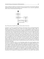
Fig. 3. Data aggregation.
Broadcast (GRAB) (Ye et al., 2005), and Energy Aware Routing (EAR) (Raghavendra et al.,
2004); (Shah & Rabaey, 2002).
DRP targets energy efﬁciency by exploiting in-network aggregation (multiple data items are
aggregated as they are forwarded by sensor nodes). Fig. 3 shows in-network data aggregation
where se nsor node I aggregates sensed data from source nodes A, B, and C, sensor node
J aggregates sensed data from source nodes D and E, and sensor node K aggregates sensed
data from source nodes F, G, and H. The sensor node L aggregates the sensed data from sensor
nodes I, J, and K, and transmits the aggregated data to the sink node. DRP uses reverse path
forwarding where data reports (packets containing sensed data in response to query) ﬂow in
the reverse direction of the query propagation to reach the sink.
Directed diffusion targets energy efﬁciency, scalability, and robustness under network
dynamics using reverse path forwarding. Directed diffusion builds a shared mesh to deliver

data from multipl e sources to multiple sinks. The sink node disseminates the query, a process
referred to as interest propagation (Fig. 4(a)). When a sensor node receives a query from a
neighboring node, the sensor node sets up a vector called the gradient from itself to the
neighboring node and directs future data ﬂows on this gradient (Fig. 4(b)). The sink node
receives an initial batch of data reports along multiple paths and uses a mechanism called
reinforcement to select a path with the best forwarding quality (Fig. 4(c)). To handle network
dynamics such as sensor node failures, each data source ﬂoods data reports period ically at
lower rates to maintain alternate paths. Directed diffusion challenges include formation of
initial gradients and wasted energy due to redundant data ﬂows to maintain alternate p aths.
GRAd optimizes data forwarding and us es cost-ﬁeld based forwarding where the cost metric
is based on the hop count (i.e., sensor nodes closer to the sink node have smaller costs and
those farther away have higher costs). The sink node ﬂoods a REQUEST message and the data
source broadcasts the d ata report containing the requested sensed information. The neighbors
with smaller costs forward the report to the sink node. GRAd drawbacks include wasted
energy due to redundant data report copies reaching the sink node.
GRAB optimizes data forwarding and uses cost-ﬁeld based for warding where the cost metric
denotes the total energy required to send a p acket to the sink node. GRAB was designed for
harsh environments with high channel error rate and frequent sensor node failures. GRAB
controls redundancy by controlling the width (number of routes from the source sensor node
Optimization Approaches in Wireless Sensor Networks 321
packet (Stojmenovi´c, 2005). Experiments conducted on Rene Motes (Culler et al., 2002) for a
trafﬁc load comprising of s ent messages every 1-10 seconds revealed that a IEEE 802.11-based
MAC consumed 2x to 6x more energy than S-MAC (Ye et al., 2004).
T-MAC adjusts the duty cycle dynamically for power efﬁcient operation. T-MAC allows a
variable sleep-sense duty cycle as opposed to the ﬁxed duty cycle used in S-MAC (e.g., 10%
sense and 90% sleep). The dynamic duty cycle further reduces the idle listening period. The
sensor node switches to s leep mode when there is no activation event ( e.g., data reception,
timer expiration, communication activity sensing, or impending data reception knowledge
through neighbors’ RTS/CTS) for a predeter mined period of time. Experimental results
obtained from T-MAC protocol implementation on OMNeT++ (Varga, 2001) to model EYES

sensor nodes (EYES, 2010) revealed that under homogeneous load (sensor nodes sent packets
with 20- to 100-byte payloads to their neighbors at random), both T-MAC and S-MAC yielded
98% energy savings as compared to CSMA whereas T-MAC o utperformed S-MAC by 5x
under variable load (Raghavendra et al., 2004).
B-MAC adjusts the duty cycle for power conservation using channel assessment information.
B-MAC duty cycles the radio through a pe riodic channel sampling mechanism k nown as low
power listening (LPL). Each time a sensor node wakes up, the sensor node turns on the radio
and checks for channel activity. If the sensor node detects activity, the sensor node powers
up and stays awake for the time required to receive an incoming packet. If no packet is
received, indicating inaccurate activity detection, a time out forces the sensor node to sleep
mode. B-MAC requires an accurate clear channel assessment to achieve low power operation.
Experimental results obtained from B-MAC and S-MAC implementation on TinyOS using
Mica2 motes revealed that B-MAC power consumption was within 25% of S-MAC for low
throughputs (below 45 bits per second) whereas B-MAC outperformed S-MAC by 60% for
higher throughputs. Results indicated that B-MAC performed better than S-MAC fo r latencies
under 6 seconds whereas S-MAC yielded lower power consumption as latency approached
10 seconds (Polastre et al., 2004).
5. Network-level Data Dissemination and Routing Protocol Optimizations
One commonality across diverse WSN application domains is the sensor node’s task to sense
and collect data about a phenomenon and transmit the data to the sink node. To meet
application requirements, this data dissemination requires energy-efﬁcient routing protocols
to establish communication paths between the sensor nodes and the sink. Typically harsh
operating environments coupled with stringent resource and energy constraints make data
dissemination and routing challenging for WSNs. Ideally, data dissemination and routing
protocols should target energy efﬁciency, robustness, and s calability. To achieve these
optimization objectives, routing protocols adjust transmission power, routing strategies, and
leverage either single-hop or multi-hop routing. In this section, we discuss protocols, which
optimize data dissemination and routing in WSNs.
5.1 Query Dissemination Optimizations
Query dissemination (transmission of a sensed d ata query/request from a sink node to a

sensor node) and data forwarding (transmission of sensed data from a sensor node to a sink
node) requires routing layer optimizations. Protocols that optimize query dissemination and
data forwarding include Declarative Routing Protocol (DRP) (Cofﬁn et al., 2000), di rected
diffusion (Intanagonwiwat et al., 2003), GRAdient Routing (GR Ad) ( Po or, 2010), GRAdient
Fig. 3. Data aggregation.
Broadcast (GRAB) (Ye et al., 2005), and Energy Aware Routing (EAR) (Raghavendra et al.,
2004); (Shah & Rabaey, 2002).
DRP targets energy efﬁciency by exploiting in-network aggregation (multiple data items are
aggregated as they are forwarded by sensor nodes). Fig. 3 shows in-network data aggregation
where se nsor node I aggregates sensed data from source nodes A, B, and C, sensor node
J aggregates sensed data from source nodes D and E, and sensor node K aggregates sensed
data from source nodes F, G, and H. The sensor node L aggregates the sensed data from sensor
nodes I, J, and K, and transmits the aggregated data to the sink node. DRP uses reverse path
forwarding where data reports (packets containing sensed data in response to query) ﬂow in
the reverse direction of the query propagation to reach the sink.
Directed diffusion targets energy efﬁciency, scalability, and robustness under network
dynamics using reverse path forwarding. Directed diffusion builds a shared mesh to deliver
data from multipl e sources to multiple sinks. The sink node disseminates the query, a process
referred to as interest propagation (Fig. 4(a)). When a sensor nod e receives a query from a
neighboring node, the sensor node sets up a vector called the gradient from itself to the
neighboring node and directs future data ﬂows on this gradient (Fig. 4(b)). The sink node
receives an initial batch of data reports along multiple paths and uses a mechanism called
reinforcement to select a path with the best forwarding quality (Fig. 4(c)). To handle network
dynamics such as sensor node failures, each data source ﬂoods data reports period ically at
lower rates to maintain alternate paths. Directed diffusion challenges include formation of
initial gradients and wasted energy due to redundant data ﬂows to maintain alternate paths.
GRAd optimizes data forwarding and uses cost-ﬁeld based for warding where the cost metric
is based on the hop count (i.e., sensor nodes closer to the sink node have smaller costs and
those farther away have higher costs). The sink node ﬂoods a REQUEST message and the data
source broadcasts the d ata report containing the requested sensed information. The neighbors

with smaller costs forward the report to the si nk node. GRAd drawbacks include wasted
energy due to redundant data report copies reaching the sink node.
GRAB optimizes data forwarding and us es cost-ﬁeld based forwarding where the cost metric
denotes the total energy required to send a packet to the sink node. GRAB was designed for
harsh environments with high channel error rate and frequent sensor node failures. GRAB
controls redundancy by controlling the width (number of routes from the source sensor node
Sustainable Wireless Sensor Networks322
Fig. 4. Directed diffusion: (a) Interest propagation; (b) Initial gradient setup; (c) Data delivery
along the reinforced path.
to the sink node) of the forwarding mesh but requires that sensor nodes make assumptions
about the energy required to transmit a data report to a neighboring node.
EAR optimizes data forwarding and uses cost-ﬁeld based forwarding where the cost
metric denotes energy per neighbor. EAR optimization objectives are load balancing and
energy conservation. EAR makes forwarding decisions probabilistically where the assigned
probability is inversely proportional to the neighbor energy cost so that paths consuming more
energy are used less frequently (Raghavendra et al., 2004).
5.2 Real-Time Constrained Optimizations
Critical WSN applications may have real-time requirements for sensed d ata d elivery
(e.g., a security/defense system monitoring enemy troops or a forest ﬁre detection
application). Failure to meet the real-time deadlines for these applications can have
catastrophic consequences. Routing protocols that consider the timing constraints for real-
time requirements include Real-time Architecture and Protocol (RAP) (Lu et al., 2002) and a
stateless protocol for real-time communication in sensor networks (SPEED) (He et al., 2003).
RAP provides real-time data delivery by considering the data report expiration time (time
after which the data is of little or no use) and the remaining distance the data report needs to
travel to reach the sink node. RAP calculates the desired velocity v
= d/t where d and t denote
the destination distance and packet lifetime, respectively. The desired velocity is updated at
each hop to reﬂect the data report’s urgency. A sensor node uses multiple ﬁrst-in-ﬁrst-out
(FIFO) queues where each queue accepts reports of velocities within a certain range and then

schedules transmissions according to a report’s degree of urgency (Raghavendra et al., 2004).
SPEED provides real-time data delivery and uses an exponentially weighted moving average
for delay calculation. Given a data report with velocity v, SPEED calculates the speed v
i
of the
report if the neighbor N
i
is selected as the next hop and then selects a neighbor with v
i
> v to
forward the report to (Rag havendra et al., 2004).
5.3 Network Topology Optimizations
Routing protocols can adjust radio transmission power to control network topology (based
on routing paths). Low-Energy Adaptive Clustering Hier archy (LEACH) (Heinzelman et al.,
2000) o p timi zes the network topology for reduced energy consumption by adjusting the
radio’s transmission power. LEACH uses a hybrid single-hop and multi-hop communication
paradigm. The sensor nodes use multi-hop communication to transmit data reports to a
cluster head (LEACH determines the cluster head using a randomized distributed algorithm).
The cluster head forwards data to the sink node using long-range radio transmission.
5.4 Resource Adaptive Optimizations
Routing protocols can adapt routing activities in accordance with available resources. Sensor
Protocols for Information via Negotiation (SPIN) (Kulik et al., 2002) optimizes performance
efﬁciency by using data negotiation and resource adaptation. In data negotiation, sensor
nodes associate metadata with nodes and exchange this metadata before actual data
transmission begins. The sensor node s interested in the data content, based on metadata,
request the actual data. This data negotiation ensures that data is sent only to interested nodes.
SPIN allows sensor nodes to adjust routing activities according to available energy resources.
At low energy levels, sensor nodes reduce or eliminate certain activities (e.g., forwarding of
metadata and data packets) (Sohraby et al., 2007).
6. Operating System-level Optimizations

A sensor node’s operating system (OS) presents optimization challenges because sensor node
operation falls between single-application devices that typically do not need an OS and
general-purpose devices with resources to run traditional embedded OSs. A sensor node’s OS
manages processor, radio, I/O buses, and Flash memory, and provides hardware abstraction
to application software, task coordination, power management, and networking services.
In this section, we discuss sever al optimizations provided by existing OSs for sensor nodes
(Sohraby et al., 2007).
6.1 Event-Driven Optimizations
Sensor nodes respond to events by controlling sensing and actuation activity. Since sensor
nodes are event-driven, it is important to optimize the OS for event handling. WSN OSs
optimized for event handling include TinyOS (TinyOS, 2010) and PicOS (Akhmetshina et al.,
2002).
TinyOS operates using an event-driven model (tasks are executed based on events). TinyOS
is written in the nesC programming language and allows application software to access
hardware directly. TinyOS’s advantages include simple OS code, energy efﬁciency, and a
small memory foot print. TinyOS challenges include introduced complexity in application
development and porting of existing C code to TinyOS.
PicOS is an event-driven OS written in C and designed for limited memory microcontrollers.
PicOS tasks are structured as a ﬁnite state machine (FSM) and state transitions are triggered
by events. PicOS is effective for reactive applications whose primary role is to react to events.
PicOS supports mul titaski ng and has small memory requirements but is not suitable for real-
time applications.
6.2 Dynamic Power Management
A sensor node’s OS can control hardware components to optimize power consumption.
Examples i nclude Operating System-directed Power Management (OSPM) (Sinha &
Chandrakasan, 2001) and MagnetOS (Barr & et al., 2002), each of which provide mechanisms
for dynamic power management. OSPM offers greedy-based dynamic power management,
which switches the sensor node to a sleep state when idle. Sleep states provide energy
conservation, however, transition to sleep state has the overhead of storing the processor
Optimization Approaches in Wireless Sensor Networks 323

Fig. 4. Directed diffusion: (a) Interest propagation; (b) Initial gradient setup; (c) Data delivery
along the reinforced path.
to the sink node) of the forwarding mesh but requires that sensor nodes make assumptions
about the energy required to transmit a data report to a neighboring node.
EAR optimizes data forwarding and uses cost-ﬁeld based forwarding where the cost
metric denotes energy per neighbor. EAR optimization objectives are load balancing and
energy conservation. EAR makes forwarding decisions probabilistically where the assigned
probability is inversely proportional to the neighbor energy cost so that paths consuming more
energy are used less frequently (Raghavendra et al., 2004).
5.2 Real-Time Constrained Optimizations
Critical WSN applications may have real-time requirements for sensed d ata d elivery
(e.g., a security/defense system monitoring enemy troops or a forest ﬁre detection
application). Failure to meet the real-time deadlines for these applications can have
catastrophic consequences. Routing protocols that consider the timing constraints for real-
time requirements include Real-time Architecture and Protocol (RAP) (Lu et al., 2002) and a
stateless protocol for real-time communication in sensor networks (SPEED) (He et al., 2003).
RAP provides real-time data delivery by considering the data report expiration time (time
after which the data is of little or no use) and the remaining distance the data report needs to
travel to reach the sink node. RAP calculates the desired velocity v
= d/t where d and t denote
the destination distance and packet lifetime, respectively. The desired velocity is updated at
each hop to reﬂect the data report’s urgency. A sensor node uses multiple ﬁrst-in-ﬁrst-out
(FIFO) queues where each queue accepts reports of velocities within a certain range and then
schedules transmissions according to a report’s degree of urgency (Raghavendra et al., 2004).
SPEED provides real-time data delivery and uses an exponentially weighted moving average
for delay calculation. Given a data report with velocity v, SPEED calculates the speed v
i
of the
report if the neighbor N
i

is selected as the next hop and then selects a neighbor with v
i
> v to
forward the report to (Rag havendra et al., 2004).
5.3 Network Topology Optimizations
Routing protocols can adjust radio transmission power to control network topology (based
on routing paths). Low-Energy Adaptive Clustering Hier archy (LEACH) (Heinzelman et al.,
2000) o p timi zes the network topology for reduced energy consumption by adjusting the
radio’s transmission power. LEACH uses a hybrid single-hop and multi-hop communication
paradigm. The sensor nodes use multi-hop communication to transmit data reports to a
cluster head (LEACH determines the cluster head using a randomized distributed algorithm).
The cluster head forwards data to the sink node using long-range radio transmission.
5.4 Resource Adaptive Optimizations
Routing protocols can adapt routing activities in accordance with available resources. Sensor
Protocols for Information via Negotiation (SPIN) (Kulik et al., 2002) optimizes performance
efﬁciency by using data negotiation and resource adaptation. In data negotiation, sensor
nodes associate metadata with nodes and exchange this metadata before actual data
transmission begins. The sensor node s interested in the data content, based on metadata,
request the actual data. This data negotiation ensures that data is sent only to interested nodes.
SPIN allows sensor nodes to adjust routing activities according to available energy resources.
At low energy levels, sensor nodes reduce or eliminate certain activities (e.g., forwarding of
metadata and data packets) (Sohraby et al., 2007).
6. Operating System-level Optimizations
A sensor node’s operating system (OS) presents optimization challenges because sensor node
operation falls between single-application devices that typically do not need an OS and
general-purpose devices with resources to run traditional embedded OSs. A sensor node’s OS
manages processor, radio, I/O buses, and Flash memory, and provides hardware abstraction
to application software, task coordination, power management, and networking services.
In this section, we discuss sever al optimizations provided by existing OSs for sensor nodes
(Sohraby et al., 2007).

6.1 Event-Driven Optimizations
Sensor nodes respond to events by controlling sensing and actuation activity. Since sensor
nodes are event-driven, it is important to optimize the OS for event handling. WSN OSs
optimized for event handling include TinyOS (TinyOS, 2010) and PicOS (Akhmetshina et al.,
2002).
TinyOS operates using an event-driven model (tasks are executed based on events). TinyOS
is written in the nesC programming language and allows application software to access
hardware directly. TinyOS’s advantages include simple OS code, energy efﬁciency, and a
small memory foot print. TinyOS challenges include introduced complexity in application
development and porting of existing C code to TinyOS.
PicOS is an event-driven OS written in C and designed for limited memory microcontrollers.
PicOS tasks are structured as a ﬁnite state machine (FSM) and state transitions are triggered
by events. PicOS is effective for reactive applications whose primary role is to react to events.
PicOS supports mul titaski ng and has small memory requirements but is not suitable for real-
time applications.
6.2 Dynamic Power Management
A sensor node’s OS can control hardware components to optimize power consumption.
Examples i nclude Operating System-directed Power Management (OSPM) (Sinha &
Chandrakasan, 2001) and MagnetOS (Barr & et al., 2002), each of which provide mechanisms
for dynamic power management. OSPM offers greedy-based dynamic power management,
which switches the sensor node to a sleep state when idle. Sleep states provide energy
conservation, however, transition to sleep state has the overhead of storing the processor
Sustainable Wireless Sensor Networks324
state and requires a ﬁnite amount of wakeup time. OSPM greedy-based adaptive sleep
mechanism disadvantages include wake up delay and potentially missing events during sleep
time. MagnetOS provides two online power-aware algorithms and an adaptive mechanism
for applications to effectively utilize the sensor node’s resources.
6.3 Fault-Tolerance
Since maintenance and repair of sensor nodes is typically not feasible after deployment, sensor
nodes require fault-tolerant mechanisms for reliable operation. MANTIS (Abrach & et al.,

2003) is a multithreaded OS that provides fault-tolerant isolation between applications by not
allowing a blocking task to prevent the execution of other tasks. In the absence of fault-tolerant
isolation, if one task executes a conditional loop whose logical condition is never satisﬁed,
then that task wil l execute in an inﬁnite loop blocking all other tasks. MANTIS facilitates
simple application development and allows dynamic reprogramming to update the sensor
node’s binary code. MANTIS offers a multimodal prototyping environment for testing WSN
applications by providing a remote shell and command server to enable inspection of the
sensor node’s memory and status remotely. MANTIS challenge s include context switch time,
stack memory overhead (since each thread requires one stack), and high energy consumption.
7. Dynamic Optimizations
Dynamic optimizations enable in-situ parameter tuning and empowers the sensor node to
adapt to changing application requirements and environmental stimuli throughout the sensor
node’s lifetime. Dynamic optimizations are important because application requirements
change over time and environmental stimuli/conditions may not be accurately predicted at
design time. Although some OS, M AC layer, and routing optimizations discussed in prior
sections of this chapter are dynamic in nature, in this section we present additional dynamic
optimization techniques for WSNs.
7.1 Dynamic Voltage and Frequency Scaling
Dynamic voltage and frequency scaling (DVFS) adjusts a sensor node’s processor voltage
and frequency to optimize energy consumption. DVFS trades off performance for reduced
energy consumption by co nsidering that the peak computation (instruction execution) rate is
much higher than the application’s average throughput requirement and that sensor nod es
are based on CMOS logic, which has a voltage dependent maximum operating frequency.
Min et al. (M in et al., 2000) demonstrated that a DVFS s ystem containing a voltage scheduler
running in tandem with the operating system’s task scheduler resulted in a 60% reduction
in energy consumption. Yuan et al. (Yuan & Qu, 2002) studied a DVFS system for sensor
nodes that required the sensor nodes to insert additional information (e.g., packet length,
expected processing time, and deadli ne) into the data packet’s header. The receiving sensor
node utilized this information to select an appropriate processor voltage and frequency to
minimize the overall energy consumption.

7.2 Software-based Dynamic Optimizations
Software can provide dy namic optimizations using techniques such as duty cycling, batching,
hierarchy, and redundancy reduction. Sof tware can control the duty cycle so that sensor
nodes are powered in a cyclic manner to reduce the average power draw. In batching,
multiple operations are buffered and then executed in a burst to reduce startup overhead cost.
Software can arrange operations in a hierarchy based on energy consumption and then invoke
low energy operations before high energy operations. Software can reduce redundancy by
compression, data aggregation, and/or message suppression. Kogekar et al. (Kogekar et al.,
2004) proposed an approach for software reconﬁguration in WSNs. The authors modeled the
WSN operation space (deﬁned by the WSN software comp onents’ models and application
requirements) and deﬁned reconﬁguration as the process of switching from one point in the
operation space to another.
7.3 Dynamic Network Reprogramming
Dynamic network reprogramming reprograms sensor nodes to change/modify tasks by
disseminating code in accordance with changing environmental stimuli. Since recollection
and reprogramming is not a feasible option for most sensor nodes, dynamic network
reprogramming enables the sensor nodes to perform different tasks. For example, a WSN
initially deployed for measuring relative humidity can measure temperature statistics after
dynamic reprogramming. The M ANTIS OS provides this dynamic reprogramming ability
(Section 6.3).
8. MDP-based Dynamic Optimizations
In this section, we extend our discussion of dynamic optimizations using an MDP-based
dynamic optimization (Munir & Gordon-Ross, 2009) as a speciﬁc example. MDP is suitable
for WSN dynamic optimizations because of MDP’s inherent ability to perform dynamic
decision making. We propose MDP as a method to perform parameter tuning-based dynamic
optimizations. Traditional microprocessor-based systems use DVFS for energy optimizations.
DVFS only provides a partial tuning for sensor nodes because sensor node s are distinct from
traditional systems i n that they have embedded sensors coupl ed with an embedded processor.
For example, the sensing frequency d ictates the amount of processed and communicated
data. We propose dynamic voltage, frequency, and sensing frequency scaling (DVFS2) to

provide enhanced optimization potential as compared to DVFS for WSNs. Our MDP-based
optimization focus es on DVFS2 but is equally applicable for extensive d esign spaces with
more tunable parameters (e.g., transmission power, packet transmiss ion interval, e tc.).
8.1 Dynamic Optimization Methodology
Fig. 5 depicts the process diagram for our dynamic optimization, which consists of three
logical domains: the application characterization domain, the communication domain, and
the sensor node tuning domain.
The application characterization domain refers to the WSN application’s
characterization/speciﬁcation where the application manager/designer (one who
manages/designs a WSN) deﬁnes various application metrics ( e.g., lifetime, throughput,
reliability, etc.) based on application requirements. The application manager/designer
also assigns weight factors to application metrics which sig nify the weightage or relative
importance of each application metric with respect to other metrics. The objective function or
reward function signiﬁes the overall reward (revenue) for given application requirements. The
application metrics along with associated weight factors represent the objective/reward function
parameters.
The communication domain (depicted by the sink node in Fig. 5) encompasses the
communication network between the application manager and the sensor nodes. The
application manager transmits the objective or reward function parameters to the sink node
via the communication domain which in turn relays these par ameters to the sensor nodes.
Optimization Approaches in Wireless Sensor Networks 325
state and requires a ﬁnite amount of wakeup time. OSPM greedy-based adaptive sleep
mechanism disadvantages include wake up delay and potentially missing events during sleep
time. MagnetOS provides two online power-aware algorithms and an adaptive mechanism
for applications to effectively utilize the sensor node’s resources.
6.3 Fault-Tolerance
Since maintenance and repair of sensor nodes is typically not feasible after deployment, sensor
nodes require fault-tolerant mechanisms for reliable operation. MANTIS (Abrach & et al.,
2003) is a multithreaded OS that provides fault-tolerant isolation between applications by not
allowing a blocking task to prevent the execution of other tasks. In the absence of fault-tolerant

isolation, if one task executes a conditional loop whose logical condition is never satisﬁed,
then that task wil l execute in an inﬁnite loop blocking all other tasks. MANTIS facilitates
simple application development and allows dynamic reprogramming to update the sensor
node’s binary code. MANTIS offers a multimodal prototyping environment for testing WSN
applications by providing a remote shell and command server to enable inspection of the
sensor node’s memory and status remotely. MANTIS challenge s include context switch time,
stack memory overhead (since each thread requires one stack), and high energy consumption.
7. Dynamic Optimizations
Dynamic optimizations enable in-situ parameter tuning and empowers the sensor node to
adapt to changing application requirements and environmental stimuli throughout the sensor
node’s lifetime. Dynamic optimizations are important because application requirements
change over time and environmental stimuli/conditions may not be accurately predicted at
design time. Although some OS, MAC layer, and routing optimizations discussed in prior
sections of this chapter are dynamic in nature, in this section we present additional dynamic
optimization techniques for WSNs.
7.1 Dynamic Voltage and Frequency Scaling
Dynamic voltage and frequency scaling (DVFS) adjusts a sensor node’s processor voltage
and frequency to optimize energy consumption. DVFS trades off performance for reduced
energy consumption by co nsidering that the peak computation (instruction execution) rate is
much higher than the application’s average throughput requirement and that sensor nod es
are based on CMOS logic, which has a voltage dependent maximum operating frequency.
Min et al. (M in et al., 2000) demonstrated that a DVFS s ystem containing a voltage scheduler
running in tandem with the operating system’s task scheduler resulted in a 60% reduction
in energy consumption. Yuan et al. (Yuan & Qu, 2002) studied a DVFS system for sensor
nodes that required the sensor nodes to insert additional information (e.g., packet length,
expected processing time, and deadli ne) into the data packet’s header. The receiving sensor
node utilized this information to select an appropriate processor voltage and frequency to
minimize the overall energy consumption.
7.2 Software-based Dynamic Optimizations
Software can provide dy namic optimizations using techniques such as duty cycling, batching,

hierarchy, and redundancy reduction. Sof tware can control the duty cycle so that sensor
nodes are powered in a cyclic manner to reduce the average power draw. In batching,
multiple operations are buffered and then executed in a burst to reduce startup overhead cost.
Software can arrange operations in a hierarchy based on energy consumption and then invoke
low energy operations before high energy operations. Software can reduce redundancy by
compression, data aggregation, and/or message suppression. Kogekar et al. (Kogekar et al.,
2004) proposed an approach for software reconﬁguration in WSNs. The authors modeled the
WSN operation space (deﬁned by the WSN software comp onents’ models and application
requirements) and deﬁned reconﬁguration as the process of switching from one point in the
operation space to another.
7.3 Dynamic Network Reprogramming
Dynamic network reprogramming reprograms sensor nodes to change/modify tasks by
disseminating code in accordance with changing environmental stimuli. Since recollection
and reprogramming is not a feasible option for most sensor nodes, dynamic network
reprogramming enables the sensor nodes to perform different tasks. For example, a WSN
initially deployed for measuring relative humidity can measure temperature statistics after
dynamic reprogramming. The M ANTIS OS provides this dynamic reprogramming ability
(Section 6.3).
8. MDP-based Dynamic Optimizations
In this section, we extend our discussion of dynamic optimizations using an MDP-based
dynamic optimization (Munir & Gordon-Ross, 2009) as a speciﬁc example. MDP is suitable
for WSN dynamic optimizations because of MDP’s inherent ability to perform dynamic
decision making. We propose MDP as a method to perform parameter tuning-based dynamic
optimizations. Traditional microprocessor-based systems use DVFS for energy optimizations.
DVFS only provides a partial tuning for sensor nodes because sensor node s are distinct from
traditional systems i n that they have embedded sensors coupl ed with an embedded processor.
For example, the sensing frequency d ictates the amount of processed and communicated
data. We propose dynamic voltage, frequency, and sensing frequency scaling (DVFS2) to
provide enhanced optimization potential as compared to DVFS for WSNs. Our MDP-based
optimization focus es on DVFS2 but is equally applicable for extensive d esign spaces with

more tunable parameters (e.g., transmission power, packet transmiss ion interval, e tc.).
8.1 Dynamic Optimization Methodology
Fig. 5 depicts the process diagram for our dynamic optimization, which consists of three
logical domains: the application characterization domain, the communication domain, and
the sensor node tuning domain.
The application characterization domain refers to the WSN application’s
characterization/speciﬁcation where the application manager/designer (one who
manages/designs a WSN) deﬁnes various application metrics ( e.g., lifetime, throughput,
reliability, etc.) based on application requirements. The application manager/designer
also assigns weight factors to application metrics which sig nify the weightage or relative
importance of each application metric with respect to other metrics. The objective function or
reward function signiﬁes the overall reward (revenue) for given application requirements. The
application metrics along with associated weight factors represent the objective/reward function
parameters.
The communication domain (depicted by the sink node in Fig. 5) encompasses the
communication network between the application manager and the sensor nodes. The
application manager transmits the objective or reward function parameters to the sink node
via the communication domain which in turn relays these par ameters to the sensor nodes.
Sustainable Wireless Sensor Networks326
Fig. 5. Process diagram for parameter tuning-based dynamic optimizations for WSNs.
The sensor node tuning domain consists of sensor nodes and performs sensor node parameter
tuning. Each sensor node contains a dynamic optimization controller, which orchestrates the
dynamic optimization process. The dynamic optimization controller module receives the
reward function parameters and invokes an online optimization algorithm to determine an
optimal or near-optimal sensor node state (tunable parameter value settings).
Our proposed methodology reacts to environmental stimuli via a dynamic proﬁler module,
which monitors environmental changes over time and captures unanticipated environmental
situations not predictable at design time. The dynamic proﬁler module proﬁles the proﬁling
statistics (e.g., wireless channel condition, number of packets dropped, battery energy, etc.).
The dynamic proﬁler module informs the dynamic optimization controller as well as the

application manager of the proﬁled statistics. The dynamic optimization controller processes
the proﬁling statistics to determine i f the current operating state meets the application
requirements. If the current operating state does not meet the application requirements,
the dynamic optimization controller reinvokes the online optimization alg orithm (e.g., MDP-
based or any other) to determine the new operating state. This feedback process continues to
ensure the selection of a good operating state to better meet application requirements in the
presence of changing environmental stimuli.
8.2 Dynamic Optimization Formulation
In this subsection, we formulate the constructs of our MDP-based dynamic optimization
(Munir & Gordon-Ross, 2009). Although we describe dynamic optimization constructs with
reference to MDP, our formulation provides insight into any other dynamic optimization
algorithm.
8.2.1 State Space
The state space S for our MDP-based dynamic optimization methodology given N tunable
parameters is deﬁned as:
where S
i
denotes the state space for tunable parameter i, ∀ i ∈ and ×
denotes the Cartesian product. The state space S consists of a total of I states as given
by the state space cardinality Each tunable parameter’s state space S
i
consists of n
tunable values:
where denotes the number of tunable values in S
i
. S is a set of N-tuples formed by taking
one tunable parameter value from each tunable parameter. A single N-tuple s
∈ S is given as:
Each N-tuple represents a sensor note state. We point out that some N-tuple s in S may not
be feasible (such as invalid combinations o f processor voltage and frequency) and can be

regarded as do not care tuples.
For example, given three tunable parameters, S can be written as:
S
= V
p
× F
p
× F
s
(4)
where V
p
, F
p
, and F
s
denote the state space for a sensor node’s processor voltage, processor
frequency, and sensing (sampling) frequency, respectively.
8.2.2 Decision Epochs and Actions
The decision epochs refe r to the points of time during a sensor node’s lifetime at which the
sensor node makes a decision regarding its operating state (i.e., whether to continue operating
in the current state or transition to another state). We consider a discrete time process where
time is divided into periods and a decision epoch correspo nds to the beginning of a period.
The sequence of decision epochs is represented as:
where the random variable N corresponds to the sensor node’s lifetime (each individual time
period in T can be denoted as time t).
At each decision epoch, a s ensor node’s action determines the next state to transition to gi ven
the current state. The sensor node action in state i
∈ S is deﬁned as:
where a

i,j
denotes the action taken at time t that causes the sensor node to transition to state j
at time t
+ 1 from the current state i. If a
i,j
= 1, the action is taken and if a
i,j
= 0, the action is
not taken.
Optimization Approaches in Wireless Sensor Networks 327
Fig. 5. Process diagram for parameter tuning-based dynamic optimizations for WSNs.
The sensor node tuning domain consists of sensor nodes and performs sensor node parameter
tuning. Each sensor node contains a dynamic optimization controller, which orchestrates the
dynamic optimization process. The dynamic optimization controller module receives the
reward function parameters and invokes an online optimization algorithm to determine an
optimal or near-optimal sensor node state (tunable parameter value settings).
Our proposed methodology reacts to environmental stimuli via a dynamic proﬁler module,
which monitors environmental changes over time and captures unanticipated environmental
situations not predictable at design time. The dynamic proﬁler module proﬁles the proﬁling
statistics (e.g., wireless channel condition, number of packets dropped, battery energy, etc.).
The dynamic proﬁler module informs the dynamic optimization controller as well as the
application manager of the proﬁled statistics. The dynamic optimization controller processes
the proﬁling statistics to determine i f the current operating state meets the application
requirements. If the current operating state does not meet the application requirements,
the dynamic optimization controller reinvokes the online optimization alg orithm (e.g., MDP-
based or any other) to determine the new operating state. This feedback process continues to
ensure the selection of a good operating state to better meet application requirements in the
presence of changing environmental stimuli.
8.2 Dynamic Optimization Formulation
In this subsection, we formulate the constructs of our MDP-based dynamic optimization

(Munir & Gordon-Ross, 2009). Although we describe dynamic optimization constructs with
reference to MDP, our formulation provides insight into any other dynamic optimization
algorithm.
8.2.1 State Space
The state space S for our MDP-based dynamic optimization methodology given N tunable
parameters is deﬁned as:
where S
i
denotes the state space for tunable parameter i, ∀ i ∈ and ×
denotes the Cartesian product. The state space S consists of a total of I states as given
by the state space cardinality Each tunable parameter’s state space S
i
consists of n
tunable values:
where denotes the number of tunable values in S
i
. S is a set of N-tuples formed by taking
one tunable parameter value from each tunable parameter. A single N-tuple s
∈ S is given as:
Each N-tuple represents a sensor note state. We point out that some N-tuple s in S may not
be feasible (such as invalid combinations of p roces sor voltage and frequency) and can be
regarded as do not care tuples.
For example, given three tunable parameters, S can be written as:
S
= V
p
× F
p
× F
s

(4)
where V
p
, F
p
, and F
s
denote the state space for a sensor node’s processor voltage, processor
frequency, and sensing (sampling) frequency, respectively.
8.2.2 Decision Epochs and Actions
The decision epochs refe r to the points of time during a sensor node’s lifetime at which the
sensor node makes a decision regarding its operating state (i.e., whether to continue operating
in the current state or transition to another state). We consider a discrete time process where
time is divided into periods and a decision epoch correspo nds to the beginning of a period.
The sequence of decision epochs is represented as:
where the random variable N corresponds to the sensor node’s lifetime (each individual time
period in T can be denoted as time t).
At each decision epoch, a s ensor node’s action determines the next state to transition to gi ven
the current state. The sensor node action in state i
∈ S is deﬁned as:
where a
i,j
denotes the action taken at time t that causes the sensor node to transition to state j
at time t
+ 1 from the current state i. If a
i,j
= 1, the action is taken and if a
i,j
= 0, the action is
not taken.

Sustainable Wireless Sensor Networks328
8.2.3 Policy and Performance Criterion
For each given state s ∈ S, a policy π determi nes whether an action a ∈ A
s
is taken or not at
a decision epoch. A performance criterion compares the performance of different policies. The
sensor node selects an action prescribed by a policy based on the sensor node’s current state.
The sensor node receives a reward r
(
X
t
, Y
t
)
as a result of selecting an action Y
t
at decision
epoch t where the random variable X
t
denotes the state at decis ion epoch t. The expected total
reward υ
π
N
(s) denotes the expected total reward over the decision making horizon N given a
speciﬁc policy π (Puterman, 2005); (Stevens-Navarro et al., 2008):
υ
π
N
(s) = lim
N→∞

E
π
s

E
N

N
∑
t=1
r(X
t
, Y
t
)

(7)
where E
π
s
represents the expected reward with respect to policy π and the initial state s (the
system state at the time of the expe cted reward calculation) and E
N
denotes the expected
reward with respect to the probability distribution of the random variable N. We can write (7)
as (Puterman, 2005):
υ
λ
N
(s) = E

π
s

∞
∑
t=1
λ
t−1
r(X
t
, Y
t
)

(8)
which gives the expected total discounted reward. We assume that the random variable N is
geometrically distributed with parameter λ and hence the distribution mean is 1/
(1 − λ)
(Stevens-Navarro et al., 2008). The parameter λ can be interpreted as a discount factor, which
measures the present value of one unit of reward received one period in the future. Thus,
υ
λ
N
(s) represents the expected total present value of the reward (income) stream obtained
using policy π (Puterman, 2005). Our objective is to ﬁnd a pol icy that maximizes the expected
total discounted reward i.e., a policy π
∗
is optimal if:
υ
π

∗
(s) ≥ υ
π
(s) ∀ π ∈ Π (9)
where Π denotes the set of admissible policies.
8.2.4 State Dynamics
The state dynamics of the system (sensor node) can be delineated by the state transition
probabilities of the embedded Markov chain. We formulate our sensor node policy as
a deterministic dynamic program (DDP) because the choice of an action deter mines the
subsequent state with certainty. Our sensor node DDP policy formulation uses a transfer
function to specify the next state. A transfer function deﬁnes a mapping τ
t
(s, a) from S × A
s
→
S, which speciﬁes the system state at time t + 1 when the sensor node selects action a ∈ A
s
in
state s at time t. To formulate our DDP as an MDP, we d eﬁne the transition probability function
as:
8.2.5 Reward Function
The reward function captures application metrics and sensor node characteristics. Our reward
function characterization considers the power consumption (which affects the sensor node
Fig. 6. Reward functions: (a) Power reward function f
p
(s, a); (b) Throughput reward function
f
t
(s, a); (c) D elay reward function f
d

(s, a).
lifetime), throughput, and delay application metrics. We deﬁne the reward function f
(s, a)
given the current sensor node state s and the sensor node’s s elected action a as:
where f
k
(s, a) and ω
k
denote the reward function and weight factor for the k
th
application
metric, respectively, given that there are m application metrics. Our objective function
characterization considers power, throughput, and delay (i.e., m
= 3) (additional application
metrics can be included) and is given as:
f
(s, a) = ω
p
f
p
(s, a) + ω
t
f
t
(s, a) + ω
d
f
d
(s, a) (12)
where f

p
(s, a) denotes the power reward function, f
t
(s, a) denotes the throughput reward
function, and f
d
(s, a) denotes the delay reward function (Fig. 6); ω
p
, ω
t
, and ω
d
represent the
weight factors for power, throughput, and delay, respectively.
We deﬁne linear reward f unctions for application metrics because an application metric
reward (objective function) typically varies linearly, or piecewise linearly, between the
minimum and maximum allowed values of the metric (Stevens-Navarro et al., 2008).
However, a non-linear characterization of reward functions is also possible and depends
upon the particular application. Our methodology works for any characterization of reward
function. We deﬁne the power reward function (Fig. 6(a)) in (11) as:
f
p
(s, a) =





1, 0
< p

a
≤ L
P
(U
P
− p
a
)/(U
P
− L
P
), L
P
< p
a
< U
P
0, p
a
≥ U
P
(13)
Optimization Approaches in Wireless Sensor Networks 329
8.2.3 Policy and Performance Criterion
For each given state s ∈ S, a policy π determi nes whether an action a ∈ A
s
is taken or not at
a decision epoch. A performance criterion compares the performance of different policies. The
sensor node selects an action prescribed by a policy based on the sensor node’s current state.
The sensor node receives a reward r

(
X
t
, Y
t
)
as a result of selecting an action Y
t
at decision
epoch t where the random variable X
t
denotes the state at decis ion epoch t. The expected total
reward υ
π
N
(s) denotes the expected total reward over the decision making horizon N given a
speciﬁc policy π (Puterman, 2005); (Stevens-Navarro et al., 2008):
υ
π
N
(s) = lim
N→∞
E
π
s

E
N

N

∑
t=1
r(X
t
, Y
t
)

(7)
where E
π
s
represents the expected reward with respect to policy π and the initial state s (the
system state at the time of the expe cted reward calculation) and E
N
denotes the expected
reward with respect to the probability distribution of the random variable N. We can write (7)
as (Puterman, 2005):
υ
λ
N
(s) = E
π
s

∞
∑
t=1
λ
t−1

r(X
t
, Y
t
)

(8)
which gives the expected total discounted reward. We assume that the random variable N is
geometrically distributed with parameter λ and hence the distribution mean is 1/
(1 − λ)
(Stevens-Navarro et al., 2008). The parameter λ can be interpreted as a discount factor, which
measures the present value of one unit of reward received one period in the future. Thus,
υ
λ
N
(s) represents the expected total present value of the reward (income) stream obtained
using policy π (Puterman, 2005). Our objective is to ﬁnd a pol icy that maximizes the expected
total discounted reward i.e., a policy π
∗
is optimal if:
υ
π
∗
(s) ≥ υ
π
(s) ∀ π ∈ Π (9)
where Π denotes the set of admissible poli ci es.
8.2.4 State Dynamics
The state dynamics of the system (sensor node) can be delineated by the state transition
probabilities of the embedded Markov chain. We formulate our sensor node policy as

a deterministic dynamic program (DDP) because the choice of an action deter mines the
subsequent state with certainty. Our sensor node DDP policy formulation uses a transfer
function to specify the next state. A transfer function deﬁnes a mapping τ
t
(s, a) from S × A
s
→
S, which speciﬁes the system state at time t + 1 when the sensor node selects action a ∈ A
s
in
state s at time t. To formulate our DDP as an MDP, we d eﬁne the transition probability function
as:
8.2.5 Reward Function
The reward function captures application metrics and sensor node characteristics. Our reward
function characterization considers the power consumption (which affects the sensor node
Fig. 6. Reward functions: (a) Power reward function f
p
(s, a); (b) Throughput reward function
f
t
(s, a); (c) D elay reward function f
d
(s, a).
lifetime), throughput, and delay application metrics. We deﬁne the reward function f
(s, a)
given the current sensor node state s and the sensor node’s s elected action a as:
where f
k
(s, a) and ω
k

denote the reward function and weight factor for the k
th
application
metric, respectively, given that there are m application metrics. Our objective function
characterization considers power, throughput, and delay (i.e., m
= 3) (additional application
metrics can be included) and is given as:
f
(s, a) = ω
p
f
p
(s, a) + ω
t
f
t
(s, a) + ω
d
f
d
(s, a) (12)
where f
p
(s, a) denotes the power reward function, f
t
(s, a) denotes the throughput reward
function, and f
d
(s, a) denotes the delay reward function (Fig. 6); ω
p

, ω
t
, and ω
d
represent the
weight factors for power, throughput, and delay, respectively.
We deﬁne linear reward f unctions for application metrics because an application metric
reward (objective function) typically varies linearly, or piecewise linearly, between the
minimum and maximum allowed values of the metric (Stevens-Navarro et al., 2008).
However, a non-linear characterization of reward functions is also possible and depends
upon the particular application. Our methodology works for any characterization of reward
function. We deﬁne the power reward function (Fig. 6(a)) in (11) as:
f
p
(s, a) =





1, 0
< p
a
≤ L
P
(U
P
− p
a
)/(U

P
− L
P
), L
P
< p
a
< U
P
0, p
a
≥ U
P
(13)
Sustainable Wireless Sensor Networks330
where p
a
denotes the power consumption of the current state given action a taken at time t and
the constant parameters L
P
and U
P
denote the minimum and maximum allowed /tolerated
sensor node power consumption, respectively. Similar equations can be written for f
t
(s, a)
and f
d
(s, a).
State transitioning incurs a cost associated with switching parameter values from the current

state to the next state (typically in the form of power and/or execution (time) overhead). We
deﬁne the transition cost function h
(s, a) as:
h
(s, a) =

H
i,a
if i = a
0 if i
= a
(14)
where H
i,a
denotes the transition cost to switch from the current state i to the next state as
determined by action a. Note that a sensor node incurs no transition cost if action a prescribes
that the next state is the same as the current state.
Hence, the overall reward function r
(s, a) given state s and action a at time t is:
r
(s, a) = f (s, a) − h(s, a) (15)
which accounts for the power, throughput, and delay application metrics as well as state
transition cost.
8.2.6 Optimality Equation
The optimality equation, also known as Bellman’s equation, for expected total discounted
reward criterion is given as (Puterman, 2005):
where υ(s) denotes the maximum expected total discounted reward. The salient properties of
the optimality equation are: the optimality equation has a unique solution; an optimal poli cy
exists given conditions on states, actions, rewards, and transition probabilities; the value of the
discounted MDP satisﬁes the optimality equation; and the optimality equation characterizes

stationary policies.
The solution of (16) gives the maximum expected total discounted reward υ
(s) and the MDP-
based optimal policy π
∗
(or π
MDP
), which gives the maximum υ(s). π
MDP
prescribes the
action a from action set A
s
given the current state s for all s ∈ S. There are several methods
to solve the optimality equation (16) such as value iteration, policy iteration, and linear
programming, however in this work we use the policy iteration algorithm. The details of
the policy iteration algorithm can be found in (Puterman, 2005).
8.3 Numerical Results
In this section, we compare the performance (based on exp ected total discounted reward
criterion) of our proposed MDP-based D V FS2 optimal policy π
∗
(π
MDP
) with several ﬁxed
heuristic policies using a representative WSN platform. We use the MATLAB MDP tool
box (Chadès et al., 2005) implementation of the pol icy iteration algorithm (Puterman, 2005)
to determine the MDP-based optimal policy. Given the reward function, sensor node state
parameters, and transition probabilities, (8) gives the expected total discounted reward. Our
reference WSN platform consists of eXtreme Scale Motes (XSM) sensor node s (Dutta et al.,
Parameter i
1

= [2.7, 2, 2] i
2
= [3, 4, 4] i
3
= [4, 6, 6] i
4
= [5.5, 8, 8]
p
i
10 units 15 units 30 units 55 units
t
i
4 units 8 units 12 units 16 units
d
i
26 units 14 units 8 units 6 units
Table 2. Power consumption p
i
, throughput t
i
, and delay d
i
parameters for wireless se nsor
node state i
= [V
p
, F
p
, F
s

] (V
p
is speciﬁed in vol ts, F
p
in MHz, and F
s
in KHz). Parameters are
speciﬁed as a multiple o f a base unit where one power unit is equal to 1 mW, one throughput
unit is equal to 0.5 MIPS, and one de lay unit is equal to 50 ms. Parameter values are based on
the XSM mote.
2005); (Dutta & Culler, 2005). The XSM motes have an average lifetime of 1,000 hours
of continuous operation with two AA alk ali ne batteries, which can deliver 6 Whr or an
average of 6 mW (Dutta et al., 2005). The XSM platform integrates an Atmel ATmega128L
microcontroller (ATMEL, 2009), a Chipcon CC1000 radio operating at 433 MHz, and a 4
Mbit serial ﬂash memory. The XSM motes contain infra red, magnetic, acoustic, photo, and
temperature s ensors. To represent sensor node operation, we analyze a sample application
domain that represents a typical security system or defense application (henceforth refer red
to as a security/defense system).
8.3.1 Fixed Heuristic Policies for Performance Comparisons
We consider the following four ﬁxed heuristic policies for comparison with our MD P policy:
• A ﬁxed heuristic policy π
POW
that always selects the state with the lowest power
consumption.
• A ﬁxed heuristic policy π
THP
that always selects the state with the highest throughput.
• A ﬁxed heuristic policy π
EQU
that spends an equal amount of time in each of the

available states.
• A ﬁxed heuristic policy π
PRF
that spends an unequal amount of time in each of the
available states based on a speciﬁed preference for each state. For example, given a
system with four possible states, the π
PRF
policy may s p end 40% of the time in the ﬁrs t
state, 20% of the time in the second state, 10% of the time in the third state, and 30% of
the time in the fourth state.
8.3.2 MDP Speciﬁcations
We compare different policies using the expected total discounted reward performance criterion.
The state transition probability for each sensor node state is given by (10). The sensor node’s
lifetime and the time between decision epochs are subjective and may be assigned by an
application manager according to application requirements. A sensor node’s mean lifetime
is given by 1/
(1 − λ) time units, which is the time between successive decision epochs (which
we assume to be 1 hour). For instance for λ
= 0.999, the s ensor node’ s mean lifetime is
1/
(1 − 0.999) = 1000 hours ≈ 42 days.
For our numerical results, we consider a sensor node capable of operating in four
different states (i.e., I
= 4 in (1)). Each state has a set of allowed actions
prescribing transitions to available states. For each allowed action a in a state, there
is a pair where r
a
speciﬁes the immediate reward obtained by taking action a
and p
a

denotes the probability of taking action a.

Sustainable Wireless Sensor Networks Part 10 docx

Tài liệu liên quan

Tài liệu bạn tìm kiếm đã sẵn sàng tải về