Climate Change and Variability Part 2 ppt

Bạn đang xem bản rút gọn của tài liệu. Xem và tải ngay bản đầy đủ của tài liệu tại đây (968.8 KB, 30 trang )

Climate Change and Variability18

regional temperature reconstructions show some agreement with the assumed low-
frequency variability in solar forcing of the last 12 centuries (Bard et al., 2000). The medieval
period, with high temperatures, had a general high solar activity, whereas the cold LIA was
dominated by lower solar activity (Ammann et al., 2007). The warming in the 20
th
century
coincides with an increase in solar forcing, although the warming trend has probably also
been amplified in the last decades by anthropogenic greenhouse gas emissions (IPCC, 2007).

4. Conclusion
The presently available palaeotemperature proxy data records do not support the
assumption that late 20
th
century temperatures exceeded those of the MWP in most regions,
although it is clear that the temperatures of the last few decades exceed those of any multi-
decadal period in the last 700–800 years. Previous conclusions (e.g., IPCC, 2007) in the
opposite direction have either been based on too few proxy records or been based on
instrumental temperatures spliced to the proxy reconstructions. It is also clear that
temperature changes, on centennial time-scales, occurred rather coherently in all the
investigated regions – Scandinavia, Siberia, Greenland, Central Europe, China, and North
America – with data coverage to enable regional reconstructions. Large-scale patterns as the
MWP, the LIA and the 20
th
century warming occur quite coherently in all the regional
reconstructions presented here but both their relative and absolute amplitude are not always
the same. Exceptional warming in the 10
th
century is seen in all six regional reconstructions.

Assumptions that, in particular, the MWP was restricted to the North Atlantic region can be
rejected. Generally, temperature changes during the past 12 centuries in the high latitudes
are larger than those in the lower latitudes and changes in annual temperatures also seem to
be larger than those of warm season temperatures. In order to truly assess the possible
global or hemispheric significance of the observed pattern, we need much more data. The
unevenly distributed palaeotemperature data coverage still seriously restricts our possibility
to set the observed 20
th
century warming in a global long-term perspective and investigate
the relative importance of natural and anthropogenic forcings behind the modern warming.

5. References
Alley, R.B., 2000: The Younger Dryas cold interval as viewed from Central Greenland.
Quaternary Science Reviews, 19: 213–226.
Ammann, C.M. and Wahl, E.R., 2007. The importance of the geophysical context in statistical
evaluations of climate reconstruction procedures. Climatic Change, 85: 71–88.
Ammann, C.M., Joos, F., Schimel, D.S., Otto-Bliesner, B.L., and Tomas, R.A., 2007: Solar
influence on climate during the past millennium: Results from transient
simulations with the NCAR Climate System Model. Proceedings of the National
Academy of Sciences, USA, 104, 3713–3718.
Andersen, K.K., Ditlevsen, P.D., Rasmussen, S.O., Clausen, H.B., Vinther, B.M., Johnsen, S.J.
and Steffensen, J.P., 2006: Retrieving a common accumulation record from
Greenland ice cores for the past 1800 years. Journal of Geophysical Research, 111:
D15106, doi:10.1029/2005JD006765.
Andreev, A. A., and Klimanov, V.A., 2000: Quantitative Holocene climatic reconstruction
from Arctic Russia. Journal of Paleolimnology, 24: 81–91.

Andreev, A.A., Klimanov, V.A., and Sulerzhitsky, L.D., 2001: Vegetation and climate history
of the Yana River lowland, Russia, during the last 6400 yr. Quaternary Science
Reviews, 20: 259–266.

Andreev, A.A., Tarasov, P.E., Siegert, C., Ebel, T., Klimanov, V.A., Melles, M., Bobrov, A.,
Dereviagin, A.Y., Lubinski, D., and Hubberten, H W., 2003: Late Pleistocene
vegetation and climate on the northern Taymyr Peninsula, Arctic Russia. Boreas,
32: 484–505.
Andreev, A.A., Tarasov, P.E., Klimanov, V.A., Melles, M., Lisitsyna, O.M., and Hubberten,
H W., 2004: Vegetation, climate changes around Lama Lake, Taymyr Peninsula,
Russia, during the Late Pleistocene and Holocene. Quaternatery International, 122:
69–84.
Andreev, A.A., Tarasov, P.E., Ilyashuk, B.P., Ilyashuk, E.A, Cremer, H., Hermichen, W D.,
Wisher, F., and Hubberten, H W., 2005: Holocene environmental history recorded
in Lake Lyadhej-To sediments, Polar Urals, Russia, Palaeogeography,
Palaeoclimatology, Palaeoecology, 223: 181–203.
Auer, I., Böhm, R., Jurkovic, A., Lipa, W., Orlik, A., Potzmann, R., Schöner, W., Ungersböck,
M., Matulla, C., Briffa, K., Jones, P.D., Efthymiadis, D., Brunetti, M., Nanni, T.,
Maugeri, M., Mercalli, L., Mestre, O., Moisselin, J M., Begert, M., Müller-
Westermeier, G., Kveton, V., Bochnicek, O., Stastny, P., Lapin, M., Szalai, S.,
Szentimrey, T., Cegnar, T., Dolinar, M., Gajic-Capka, M., Zaninovic, K.,
Majstorovic, Z., and Nieplova, E., 2007: HISTALP – Historical instrumental
climatological surface time series of the greater Alpine region 1760–2003.
Intentional Journal of Climatology 27: 17–46.
Barclay, D.J., Wiles, G.C., and Calkin, P.E. 2009. Tree-ring crossdates for a first millennium
AD advance of Tebenkof Glacier, southern Alaska. Quaternary Research, 71: 22–26.
Bard, E., Raisbeck, G., Yiou, F., and Jouzel, J., 2000: Solar irradiance during the last 1200
years based on cosmogenic nuclides. Tellus, 52B: 985–992.
Bjune, A.E., Seppä, H., and Birks, H.J.B., 2009: Quantitative summer-temperature
reconstructions for the last 2000 years based on pollen-stratigraphical data from
northern Fennoscandia. Journal of Paleolimnology, 41: 43–56.
Böhm, R., Jones, P.D., Hiebl, J., Frank, D., Brunetti, M., and Maugeri, M., 2010: The early
instrumental warm-bias: a solution for long Central European temperature series,
1760–2007. Climatic Change: in press.

Bradley, R.S., Briffa, K.R., Crowley, T.J., Hughes, M.K., Jones, P.D. and Mann, M.E., 2001:
The scope of medieval warming. Science, 292: 2011–2012.
Bradley, R.S., Hughes, M.K. and Diaz, H.F., 2003: Climate in medieval time. Science, 302:
404–405.
Briffa, K.R., 2000: Annual climate variability in the Holocene: interpreting the message of
ancient trees. Quaternary Science Reviews, 19: 87–105.
Broecker, W.S., 2001: Was the Medieval Warm Period global?. Science, 291: 1497–1499.
Brohan, P., Kennedy, J., Haris, I., Tett, S.F.B., and Jones, P.D., 2006: Uncertainty estimates in
regional and global observed temperature changes: a new dataset from 1850.
Journal of Geophysical Research, 111: D12106.
Chylek, P., Dubey, M.K., Lesins, G., 2006: Greenland warming of 1920–1930 and 1995–2005.
Geophysical Research Letters, 33: 10.1029/2006GL026510.
A regional approach to the Medieval Warm Period and the Little Ice Age 19

regional temperature reconstructions show some agreement with the assumed low-
frequency variability in solar forcing of the last 12 centuries (Bard et al., 2000). The medieval
period, with high temperatures, had a general high solar activity, whereas the cold LIA was
dominated by lower solar activity (Ammann et al., 2007). The warming in the 20
th
century
coincides with an increase in solar forcing, although the warming trend has probably also
been amplified in the last decades by anthropogenic greenhouse gas emissions (IPCC, 2007).

4. Conclusion
The presently available palaeotemperature proxy data records do not support the
assumption that late 20
th
century temperatures exceeded those of the MWP in most regions,
although it is clear that the temperatures of the last few decades exceed those of any multi-
decadal period in the last 700–800 years. Previous conclusions (e.g., IPCC, 2007) in the

opposite direction have either been based on too few proxy records or been based on
instrumental temperatures spliced to the proxy reconstructions. It is also clear that
temperature changes, on centennial time-scales, occurred rather coherently in all the
investigated regions – Scandinavia, Siberia, Greenland, Central Europe, China, and North
America – with data coverage to enable regional reconstructions. Large-scale patterns as the
MWP, the LIA and the 20
th
century warming occur quite coherently in all the regional
reconstructions presented here but both their relative and absolute amplitude are not always
the same. Exceptional warming in the 10
th
century is seen in all six regional reconstructions.
Assumptions that, in particular, the MWP was restricted to the North Atlantic region can be
rejected. Generally, temperature changes during the past 12 centuries in the high latitudes
are larger than those in the lower latitudes and changes in annual temperatures also seem to
be larger than those of warm season temperatures. In order to truly assess the possible
global or hemispheric significance of the observed pattern, we need much more data. The
unevenly distributed palaeotemperature data coverage still seriously restricts our possibility
to set the observed 20
th
century warming in a global long-term perspective and investigate
the relative importance of natural and anthropogenic forcings behind the modern warming.

5. References
Alley, R.B., 2000: The Younger Dryas cold interval as viewed from Central Greenland.
Quaternary Science Reviews, 19: 213–226.
Ammann, C.M. and Wahl, E.R., 2007. The importance of the geophysical context in statistical
evaluations of climate reconstruction procedures. Climatic Change, 85: 71–88.
Ammann, C.M., Joos, F., Schimel, D.S., Otto-Bliesner, B.L., and Tomas, R.A., 2007: Solar
influence on climate during the past millennium: Results from transient

simulations with the NCAR Climate System Model. Proceedings of the National
Academy of Sciences, USA, 104, 3713–3718.
Andersen, K.K., Ditlevsen, P.D., Rasmussen, S.O., Clausen, H.B., Vinther, B.M., Johnsen, S.J.
and Steffensen, J.P., 2006: Retrieving a common accumulation record from
Greenland ice cores for the past 1800 years. Journal of Geophysical Research, 111:
D15106, doi:10.1029/2005JD006765.
Andreev, A. A., and Klimanov, V.A., 2000: Quantitative Holocene climatic reconstruction
from Arctic Russia. Journal of Paleolimnology, 24: 81–91.

Andreev, A.A., Klimanov, V.A., and Sulerzhitsky, L.D., 2001: Vegetation and climate history
of the Yana River lowland, Russia, during the last 6400 yr. Quaternary Science
Reviews, 20: 259–266.
Andreev, A.A., Tarasov, P.E., Siegert, C., Ebel, T., Klimanov, V.A., Melles, M., Bobrov, A.,
Dereviagin, A.Y., Lubinski, D., and Hubberten, H W., 2003: Late Pleistocene
vegetation and climate on the northern Taymyr Peninsula, Arctic Russia. Boreas,
32: 484–505.
Andreev, A.A., Tarasov, P.E., Klimanov, V.A., Melles, M., Lisitsyna, O.M., and Hubberten,
H W., 2004: Vegetation, climate changes around Lama Lake, Taymyr Peninsula,
Russia, during the Late Pleistocene and Holocene. Quaternatery International, 122:
69–84.
Andreev, A.A., Tarasov, P.E., Ilyashuk, B.P., Ilyashuk, E.A, Cremer, H., Hermichen, W D.,
Wisher, F., and Hubberten, H W., 2005: Holocene environmental history recorded
in Lake Lyadhej-To sediments, Polar Urals, Russia, Palaeogeography,
Palaeoclimatology, Palaeoecology, 223: 181–203.
Auer, I., Böhm, R., Jurkovic, A., Lipa, W., Orlik, A., Potzmann, R., Schöner, W., Ungersböck,
M., Matulla, C., Briffa, K., Jones, P.D., Efthymiadis, D., Brunetti, M., Nanni, T.,
Maugeri, M., Mercalli, L., Mestre, O., Moisselin, J M., Begert, M., Müller-
Westermeier, G., Kveton, V., Bochnicek, O., Stastny, P., Lapin, M., Szalai, S.,
Szentimrey, T., Cegnar, T., Dolinar, M., Gajic-Capka, M., Zaninovic, K.,
Majstorovic, Z., and Nieplova, E., 2007: HISTALP – Historical instrumental

climatological surface time series of the greater Alpine region 1760–2003.
Intentional Journal of Climatology 27: 17–46.
Barclay, D.J., Wiles, G.C., and Calkin, P.E. 2009. Tree-ring crossdates for a first millennium
AD advance of Tebenkof Glacier, southern Alaska. Quaternary Research, 71: 22–26.
Bard, E., Raisbeck, G., Yiou, F., and Jouzel, J., 2000: Solar irradiance during the last 1200
years based on cosmogenic nuclides. Tellus, 52B: 985–992.
Bjune, A.E., Seppä, H., and Birks, H.J.B., 2009: Quantitative summer-temperature
reconstructions for the last 2000 years based on pollen-stratigraphical data from
northern Fennoscandia. Journal of Paleolimnology, 41: 43–56.
Böhm, R., Jones, P.D., Hiebl, J., Frank, D., Brunetti, M., and Maugeri, M., 2010: The early
instrumental warm-bias: a solution for long Central European temperature series,
1760–2007. Climatic Change: in press.
Bradley, R.S., Briffa, K.R., Crowley, T.J., Hughes, M.K., Jones, P.D. and Mann, M.E., 2001:
The scope of medieval warming. Science, 292: 2011–2012.
Bradley, R.S., Hughes, M.K. and Diaz, H.F., 2003: Climate in medieval time. Science, 302:
404–405.
Briffa, K.R., 2000: Annual climate variability in the Holocene: interpreting the message of
ancient trees. Quaternary Science Reviews, 19: 87–105.
Broecker, W.S., 2001: Was the Medieval Warm Period global?. Science, 291: 1497–1499.
Brohan, P., Kennedy, J., Haris, I., Tett, S.F.B., and Jones, P.D., 2006: Uncertainty estimates in
regional and global observed temperature changes: a new dataset from 1850.
Journal of Geophysical Research, 111: D12106.
Chylek, P., Dubey, M.K., Lesins, G., 2006: Greenland warming of 1920–1930 and 1995–2005.
Geophysical Research Letters, 33: 10.1029/2006GL026510.
Climate Change and Variability20

Cook, E.R., Esper, J. and D’Arrigo, R.D., 2004: Extra-tropical Northern Hemisphere land
temperature variability over the past 1000 years. Quaternary Science Reviews, 23:
2063–2074.
Cook, T.L., Bradley, R.S., Stoner, J.S. and Francus, P., 2009: Five thousand years of sediment

transfer in a high arctic watershed recorded in annually laminated sediments from
Lower Murray Lake, Ellesmere Island, Nunavut, Canada. Journal of
Paleolimnology, 41: 77–94.
Cremer, H., Wagner, B., Melles, M., and Hubberten, H W., 2001: The postglacial
environmental development of Raffles Sø, East Greenland: inferences from a 10,000
year diatom record. Journal of Paleolimnology, 26: 67–87.
Cronin, T. M., Dwyer, G.S., Kamiya, T., Schwede, S., and Willard, D.A., 2003: Medieval
Warm Period, Little Ice Age and 20th century temperature variability from
Chesapeake Bay. Global and Planetary Change, 36: 17–29.
Crowley, T.J., 2000: Causes of climate change over the past 1000 years. Science, 289: 270–277.
Crowley, T.J. and Lowery, T., 2000: How warm was the Medieval Warm Period? A comment
on “man-made versus natural climate change”. Ambio, 29: 51–54.
Crowley, T.J., Baum, S.K., Kim, K Y., Hegerl, G.C. and Hyde, W.T., 2003: Modeling ocean
heat content changes during the last millennium. Geophysical Research Letters, 30:
1932, doi:10.1029/2003GL017801.
Dahl-Jensen, D., Mosegaard, K., Gundestrup, N., Clow, G.D., Johnsen, S.J., Hansen, A.W.,
and Balling, N., 1998: Past temperatures directly from the Greenland Ice Sheet.
Science, 282: 268–271.
D’Arrigo, R., Jacoby, G., Frank, D., Pederson, N., Cook, E., Buckley, B., Nachin, B., Mijiddorj,
R., and Dugarjav, C., 2001: 1738 years of Mongolian temperature variability
inferred from a tree-ring width chronology of Siberian pine. Geophysical Research
Letters, 28: 543–546.
D’Arrigo, R., Wilson, R. and Jacoby, G., 2006: On the long-term context for late 20
th
century
warming. Journal of Geophysical Research, 111: D3, D03103.
Dansgaard, W., Johnsen S.J., Reeh N., Gundestrup, N., Clausen, H.B., and Hammer, C.U.,
1975: Climatic changes, Norsemen and modern man. Nature, 255: 24–28.
Esper, J., Cook, E.R. and Schweingruber, F.H., 2002a: Low-frequency signals in long tree-
ring chronologies for reconstructing past temperature variability. Science, 295:

2250–2253.
Esper, J., Schweingruber, F.H. and Winiger, M., 2002b: 1300 years of climatic history for
Western Central Asia inferred from tree-rings. The Holocene, 12: 267–277.
Esper, J., Frank, D.C., Wilson, R.J.S. and Briffa, K.R., 2005a: Effect of scaling and regression
on reconstructed temperature amplitude for the past millennium. Geophysical
Research Letters, 32: L07711.
Esper, J., Wilson, R.J.S., Frank, D.C., Moberg, A., Wanner, H. and Luterbacher, J., 2005b:
Climate: past ranges and future changes. Quaternary Science Reviews, 24: 2164–
2166.
Esper, J. and Frank, D.C., 2009: IPCC on heterogeneous Medieval Warm Period. Climatic
Change, 94: 267–273.

Filippi, M.L., Lambert, P., Hunziker, J., Kubler, B., and Bernasconi, S., 1999: Climatic and
anthropogenic influence on the stable isotope record from bulk carbonates and
ostracodes in Lake Neuchatel, Switzerland, during the last two millennia. Journal
of Paleolimnology, 21: 19–34.
Fisher, D.A., Koerner, R.M., Paterson, W.S.B., Dansgaard, W., Gundestrup, N. and Reeh, N.,
1983: Effect of wind scouring on climatic records from icecore oxygen isotope
profiles. Nature, 301: 205–209.
Fricke, H.C., O’Neil, J.R., and Lynnerup, N., 1995: Oxygen isotope composition of human
tooth enamel from medieval Greenland: Linking climate and society. Geology, 23:
869–872.
Gagen, M., McCarrol, D., and Hicks, S., 2006: The Millennium project: European climate of
the last. PAGES News, 14: 4.
Ge, Q., Zheng, J., Fang, X., Man, Z., Zhang, X., Zhang, P., and Wang, W C., 2003: Winter
half-year temperature reconstruction for the middle and lower reaches of the
Yellow River and Yangtze River, China, during the past 2000 years. The Holocene,
13: 933–940.
Ge, Q.S., Zheng, J Y., Hao, Z X., Shao, X M., Wang, W C., and Luterbacher, J., 2010:
Temperature variation through 2000 years in China: An uncertainty analysis of

reconstruction and regional difference. Geophysical Research Letters, 37:
10.1029/2009GL041281.
Grove, J.M., 1988. The Little Ice Age. London, Methuen: 498 pp.
Grudd, H., 2008: Torneträsk tree-ring width and density AD 500–2004: a test of climatic
sensitivity and a new 1500-year reconstruction of north Fennoscandian summers.
Climate Dynamics, 31: 843–857.
He, Y., Theakstone, W., Zhang, Z., Zhang, D., Yao, T., Chen, T., Shen, Y., and Pang, H., 2004:
Asynchronous Holocene climatic change across China. Quaternary Research, 61:
52–63.
Hegerl, G., Crowley, T., Allen, M., Hyde, W., Pollack, H., Smerdon, J. and Zorita, E., 2007:
Detection of human influence on a new, validated, 1500 year temperature
reconstruction. Journal of Climate, 20: 650–666.
Hu, F.S., Ito, E., Brown, T.A., Curry, B.B., and Engstrom, D.R., 2001: Pronounced climatic
variations in Alaska during the last two millennia. Proceedings of the National
Academy of Sciences, USA, 98: 10552–10556.
Hu, C., Henderson, G.M., Huang, J., Xie, S., Sun, Y., and Johnson, K.R. 2008: Quantification
of Holocene Asian monsoon rainfall from spatially separated cave records. Earth
and Planetary Science Letters, 266: 221–232.
Hughes, M.K. and Diaz, H.F., 1994: Was there a ‘medieval warm period’, and if so, where
and when?. Climatic Change, 26, 109–142.
IPCC, 2007: Climate Change 2007: The physical science basis. Contribution of working
group I to the fourth assessment report of the Intergovernmental Panel on Climate
Change [Solomon, S., Qin, D., Manning, M., Chen, Z., Marquis, M., Averyt, K.B.,
Tignor, M. and Miller, H.L. (eds.)]. Cambridge and New York: Cambridge
University Press: 996 pp.
Jennings, A.E., and Weiner, N.J., 1996: Environmental change in eastern Greenland during
the last 1300 years: evidence from foraminifera and lithofacies in Nansen Fjord,
68°N. The Holocene, 6: 179–191.
A regional approach to the Medieval Warm Period and the Little Ice Age 21

Cook, E.R., Esper, J. and D’Arrigo, R.D., 2004: Extra-tropical Northern Hemisphere land
temperature variability over the past 1000 years. Quaternary Science Reviews, 23:
2063–2074.
Cook, T.L., Bradley, R.S., Stoner, J.S. and Francus, P., 2009: Five thousand years of sediment
transfer in a high arctic watershed recorded in annually laminated sediments from
Lower Murray Lake, Ellesmere Island, Nunavut, Canada. Journal of
Paleolimnology, 41: 77–94.
Cremer, H., Wagner, B., Melles, M., and Hubberten, H W., 2001: The postglacial
environmental development of Raffles Sø, East Greenland: inferences from a 10,000
year diatom record. Journal of Paleolimnology, 26: 67–87.
Cronin, T. M., Dwyer, G.S., Kamiya, T., Schwede, S., and Willard, D.A., 2003: Medieval
Warm Period, Little Ice Age and 20th century temperature variability from
Chesapeake Bay. Global and Planetary Change, 36: 17–29.
Crowley, T.J., 2000: Causes of climate change over the past 1000 years. Science, 289: 270–277.
Crowley, T.J. and Lowery, T., 2000: How warm was the Medieval Warm Period? A comment
on “man-made versus natural climate change”. Ambio, 29: 51–54.
Crowley, T.J., Baum, S.K., Kim, K Y., Hegerl, G.C. and Hyde, W.T., 2003: Modeling ocean
heat content changes during the last millennium. Geophysical Research Letters, 30:
1932, doi:10.1029/2003GL017801.
Dahl-Jensen, D., Mosegaard, K., Gundestrup, N., Clow, G.D., Johnsen, S.J., Hansen, A.W.,
and Balling, N., 1998: Past temperatures directly from the Greenland Ice Sheet.
Science, 282: 268–271.
D’Arrigo, R., Jacoby, G., Frank, D., Pederson, N., Cook, E., Buckley, B., Nachin, B., Mijiddorj,
R., and Dugarjav, C., 2001: 1738 years of Mongolian temperature variability
inferred from a tree-ring width chronology of Siberian pine. Geophysical Research
Letters, 28: 543–546.
D’Arrigo, R., Wilson, R. and Jacoby, G., 2006: On the long-term context for late 20
th
century
warming. Journal of Geophysical Research, 111: D3, D03103.

Dansgaard, W., Johnsen S.J., Reeh N., Gundestrup, N., Clausen, H.B., and Hammer, C.U.,
1975: Climatic changes, Norsemen and modern man. Nature, 255: 24–28.
Esper, J., Cook, E.R. and Schweingruber, F.H., 2002a: Low-frequency signals in long tree-
ring chronologies for reconstructing past temperature variability. Science, 295:
2250–2253.
Esper, J., Schweingruber, F.H. and Winiger, M., 2002b: 1300 years of climatic history for
Western Central Asia inferred from tree-rings. The Holocene, 12: 267–277.
Esper, J., Frank, D.C., Wilson, R.J.S. and Briffa, K.R., 2005a: Effect of scaling and regression
on reconstructed temperature amplitude for the past millennium. Geophysical
Research Letters, 32: L07711.
Esper, J., Wilson, R.J.S., Frank, D.C., Moberg, A., Wanner, H. and Luterbacher, J., 2005b:
Climate: past ranges and future changes. Quaternary Science Reviews, 24: 2164–
2166.
Esper, J. and Frank, D.C., 2009: IPCC on heterogeneous Medieval Warm Period. Climatic
Change, 94: 267–273.

Filippi, M.L., Lambert, P., Hunziker, J., Kubler, B., and Bernasconi, S., 1999: Climatic and
anthropogenic influence on the stable isotope record from bulk carbonates and
ostracodes in Lake Neuchatel, Switzerland, during the last two millennia. Journal
of Paleolimnology, 21: 19–34.
Fisher, D.A., Koerner, R.M., Paterson, W.S.B., Dansgaard, W., Gundestrup, N. and Reeh, N.,
1983: Effect of wind scouring on climatic records from icecore oxygen isotope
profiles. Nature, 301: 205–209.
Fricke, H.C., O’Neil, J.R., and Lynnerup, N., 1995: Oxygen isotope composition of human
tooth enamel from medieval Greenland: Linking climate and society. Geology, 23:
869–872.
Gagen, M., McCarrol, D., and Hicks, S., 2006: The Millennium project: European climate of
the last. PAGES News, 14: 4.
Ge, Q., Zheng, J., Fang, X., Man, Z., Zhang, X., Zhang, P., and Wang, W C., 2003: Winter
half-year temperature reconstruction for the middle and lower reaches of the

Yellow River and Yangtze River, China, during the past 2000 years. The Holocene,
13: 933–940.
Ge, Q.S., Zheng, J Y., Hao, Z X., Shao, X M., Wang, W C., and Luterbacher, J., 2010:
Temperature variation through 2000 years in China: An uncertainty analysis of
reconstruction and regional difference. Geophysical Research Letters, 37:
10.1029/2009GL041281.
Grove, J.M., 1988. The Little Ice Age. London, Methuen: 498 pp.
Grudd, H., 2008: Torneträsk tree-ring width and density AD 500–2004: a test of climatic
sensitivity and a new 1500-year reconstruction of north Fennoscandian summers.
Climate Dynamics, 31: 843–857.
He, Y., Theakstone, W., Zhang, Z., Zhang, D., Yao, T., Chen, T., Shen, Y., and Pang, H., 2004:
Asynchronous Holocene climatic change across China. Quaternary Research, 61:
52–63.
Hegerl, G., Crowley, T., Allen, M., Hyde, W., Pollack, H., Smerdon, J. and Zorita, E., 2007:
Detection of human influence on a new, validated, 1500 year temperature
reconstruction. Journal of Climate, 20: 650–666.
Hu, F.S., Ito, E., Brown, T.A., Curry, B.B., and Engstrom, D.R., 2001: Pronounced climatic
variations in Alaska during the last two millennia. Proceedings of the National
Academy of Sciences, USA, 98: 10552–10556.
Hu, C., Henderson, G.M., Huang, J., Xie, S., Sun, Y., and Johnson, K.R. 2008: Quantification
of Holocene Asian monsoon rainfall from spatially separated cave records. Earth
and Planetary Science Letters, 266: 221–232.
Hughes, M.K. and Diaz, H.F., 1994: Was there a ‘medieval warm period’, and if so, where
and when?. Climatic Change, 26, 109–142.
IPCC, 2007: Climate Change 2007: The physical science basis. Contribution of working
group I to the fourth assessment report of the Intergovernmental Panel on Climate
Change [Solomon, S., Qin, D., Manning, M., Chen, Z., Marquis, M., Averyt, K.B.,
Tignor, M. and Miller, H.L. (eds.)]. Cambridge and New York: Cambridge
University Press: 996 pp.
Jennings, A.E., and Weiner, N.J., 1996: Environmental change in eastern Greenland during

the last 1300 years: evidence from foraminifera and lithofacies in Nansen Fjord,
68°N. The Holocene, 6: 179–191.
Climate Change and Variability22

Jensen, K.G., Kuijpers, A., Koç, N., and Heinemeier, J., 2004: Diatom evidence of
hydrografhic changes and ice conditions in Igaliku Fjord, South Greenland, during
the past 1500 years. The Holocene, 14: 152–164.
Jones, P.D., Briffa, K.R., Barnett, T.P. and Tett, S.F.B., 1998: High-resolution palaeoclimatic
records for the last millennium: interpretation, integration and comparison with
General Circulation Model control-run temperatures. The Holocene, 8: 455–471.
Jones, P.D., Osborn, T.J. and Briffa, K.R., 2001: The evolution of climate over the last
millennium. Science, 292: 662–667.
Jones, P.D. and Mann, M.E., 2004: Climate over past millennia. Reviews of Geophysics, 42:
RG2002.
Jones, P.D., Briffa, K.R., Osborn, T.J., Lough, J.M., van Ommen, T.D., Vinther, B.M.,
Luterbacher, J., Wahl, E.R., Zwiers, F.W., Mann, M.E., Schmidt, G.A., Ammann,
C.M., Buckley, B.M., Cobb, K.M., Esper, J., Goosse, H., Graham, N., Jansen, E.,
Kiefer, T., Kull, C., Küttel, M., Mosley-Thompson, E., Overpeck, J.T., Riedwyl, N.,
Schulz, M., Tudhope, A.W., Villalba, R., Wanner, H., Wolff, E. and Xoplaki, E.,
2009: High-resolution palaeoclimatology of the last millennium: A review of
current status and future prospects. The Holocene, 19: 3–49.
Juckes, M.N., Allen, M.R., Briffa, K.R., Esper, J., Hegerl, G.C., Moberg, A., Osborn, T.J. and
Weber, S.L., 2007: Millennial temperature reconstruction intercomparison and
evaluation. Climate of the Past, 3: 591–609.
Kaplan, M.R., Wolfe, A.P. and Miller, G.H., 2002: Holocene environmental variability in
southern Greenland inferred from lake sediments. Quaternary Research, 58: 149–
159.
Kaufman, D.S., Schneider, D.P., McKay, N.P., Ammann, C.M., Bradley, R.S., Briffa K.R.,
Miller, G.H., Otto-Bliesner, B.L., Overpeck, J.T., Vinther, B.M., Arctic Lakes 2k
Project Members (Abbott, M., Axford, Y., Bird, B., Birks, H.J.B., Bjune, A.E., Briner,

J., Cook, T., Chipman, M., Francus, P., Gajewski, K., Geirsdóttir, Á., Hu, F.S.,
Kutchko, B., Lamoureux, S., Loso, M., MacDonald, G., Peros, M., Porinchu, D.,
Schiff, C., Seppä, H. and Thomas, E.)., 2009. Recent warming reverses long-term
Arctic cooling. Science, 325: 1236–1239.
Korhola, A., Weckström, J., Holmström, L., and Erästö, P.A., 2000: A quantitative Holocene
climatic record from diatoms in northern Fennoscandia. Quaternary Research, 54:
284–294.
Lamb, H.H., 1977: Climate: Present, past and future 2. Climatic history and the future.
London, Methuen: 835 pp.
Larocque, I., Grosjean, M., Heiri, O., Bigler, C., and Blass, A., 2009: Comparison between
chironomid-inferred July temperatures and meteorological data AD 1850–2001
from varved Lake Silvaplana, Switzerland. Journal of Paleolimnology, 41: 329–342.
Lee, T.C.K., Zwiers, F.W., and Tsao, M., 2008: Evaluation of proxy-based millennial
reconstruction methods. Climate Dynamics, 31: 263–281.
Linderholm, H.W., and Gunnarson, B.E., 2005: Summer temperature variability in central
Scandinavia during the last 3600 years. Geografiska Annaler, 87A: 231–241.
Liu, Z., Henderson, A.C.G., and Huang, Y., 2006: Alkenone-based reconstruction of late-
Holocene surface temperature and salinity changes in Lake Qinghai, China.
Geophysical Research Letters, 33: 10.1029/2006GL026151.

Ljungqvist, F.C., 2009: Temperature proxy records covering the last two millennia: a tabular
and visual overview. Geografiska Annaler, 91A: 11–29.
Ljungqvist, F.C., 2010: An improved reconstruction of temperature variability in the extra-
tropical Northern Hemisphere during the last two millennia. Geografiska Annaler,
92A: in press.
Loehle, C., 2007: A 2000-year global temperature reconstruction based on non-treering
proxies. Energy & Environment, 18: 1049–1058.
Loehle, C., 2009: A mathematical analysis of the divergence problem in dendroclimatology.
Climatic Change, 94: 233–245.
Loso, M.G., 2009: Summer temperatures during the Medieval Warm Period and Little Ice

Age inferred from varved proglacial lake sediments in southern Alaska. Journal of
Paleolimnology, 41: 117–128.
Luckman, B.H., and Wilson, R.J.S., 2005: Summer temperatures in the Canadian Rockies
during the last millennium: a revised record. Climate Dynamics, 24: 131–144.
Mangini, A., Spötl, C., and Verdes, P., 2005: Reconstruction of temperature in the Central
Alps during the past 2000 yr from a δ
18
O stalagmite record. Earth and Planetary
Science Letters, 235: 741–751.
Mann, M.E., Bradley, R.S. and Hughes, M.K., 1998: Global-scale temperature patterns and
climate forcing over the past six centuries. Nature, 392: 779–787.
Mann, M.E., Bradley, R.S. and Hughes, M.K., 1999: Northern hemisphere temperatures
during the past millennium: inferences, uncertainties, and limitations. Geophysical
Research Letters, 26: 759–762.
Mann, M.E. and Jones, P.D., 2003: Global surface temperatures over the past two millennia.
Geophysical Research Letters, 30: 1820.
Mann, M.E., Cane, M.A., Zebiak, S.E. and Clement, A., 2005: Volcanic and Solar Forcing of
the Tropical Pacific over the Past 1000 Years. Journal of Climate, 18: 417–456.
Mann, M.E., Zhang, Z., Hughes, M.K., Bradley, R.S., Miller, S.K., Rutherford, S. and Ni, F.,
2008: Proxy-based reconstructions of hemispheric and global surface temperature
variations over the past two millennia. Proceedings of the National Academy of
Sciences, USA, 105: 13252–13257.
Mann, M.E., Zhang, Z., Rutherford, S., Bradley, R.S., Hughes, M.K., Shindell, D., Ammann,
C., Faluvegi, G., and Ni, F., 2009: Global signatures and dynamical origins of the
Little Ice Age and Medieval Climate Anomaly. Science, 326: 1256–1260.
Matthews, J.A., and Briffa, K.R., 2005: The ‘Little Ice Age’: Re-evaluation of an evolving
concept. Geografiska Annaler, 87A: 17–36.
Moberg, A., Sonechkln, D.M., Holmgren, K., Datsenko, N.M., and Karlén, W., 2005: Highly
variable Northern Hemisphere temperatures reconstructed from low- and high-
resolution proxy data. Nature, 433: 613–617.

Moros, M., Jensen, K.G., and Kuijpers, A., 2006: Mid- to late-Holocene hydrological and
climatic variability in Disko Bugt, central West Greenland. The Holocene, 16: 357–
67.
Møller, H.S., Jensen, K.G., Kuijpers, A., Aagaard-Sørensen, S., Seidenkrantz, M.S., Prins, M.,
Endler, R., and Mikkelsen, N., 2006: Late-Holocene environment and climatic
changes in Ameralik Fjord, southwest Greenland: evidence from the sedimentary
record. The Holocene, 16: 685–95.
A regional approach to the Medieval Warm Period and the Little Ice Age 23

Jensen, K.G., Kuijpers, A., Koç, N., and Heinemeier, J., 2004: Diatom evidence of
hydrografhic changes and ice conditions in Igaliku Fjord, South Greenland, during
the past 1500 years. The Holocene, 14: 152–164.
Jones, P.D., Briffa, K.R., Barnett, T.P. and Tett, S.F.B., 1998: High-resolution palaeoclimatic
records for the last millennium: interpretation, integration and comparison with
General Circulation Model control-run temperatures. The Holocene, 8: 455–471.
Jones, P.D., Osborn, T.J. and Briffa, K.R., 2001: The evolution of climate over the last
millennium. Science, 292: 662–667.
Jones, P.D. and Mann, M.E., 2004: Climate over past millennia. Reviews of Geophysics, 42:
RG2002.
Jones, P.D., Briffa, K.R., Osborn, T.J., Lough, J.M., van Ommen, T.D., Vinther, B.M.,
Luterbacher, J., Wahl, E.R., Zwiers, F.W., Mann, M.E., Schmidt, G.A., Ammann,
C.M., Buckley, B.M., Cobb, K.M., Esper, J., Goosse, H., Graham, N., Jansen, E.,
Kiefer, T., Kull, C., Küttel, M., Mosley-Thompson, E., Overpeck, J.T., Riedwyl, N.,
Schulz, M., Tudhope, A.W., Villalba, R., Wanner, H., Wolff, E. and Xoplaki, E.,
2009: High-resolution palaeoclimatology of the last millennium: A review of
current status and future prospects. The Holocene, 19: 3–49.
Juckes, M.N., Allen, M.R., Briffa, K.R., Esper, J., Hegerl, G.C., Moberg, A., Osborn, T.J. and
Weber, S.L., 2007: Millennial temperature reconstruction intercomparison and
evaluation. Climate of the Past, 3: 591–609.
Kaplan, M.R., Wolfe, A.P. and Miller, G.H., 2002: Holocene environmental variability in

southern Greenland inferred from lake sediments. Quaternary Research, 58: 149–
159.
Kaufman, D.S., Schneider, D.P., McKay, N.P., Ammann, C.M., Bradley, R.S., Briffa K.R.,
Miller, G.H., Otto-Bliesner, B.L., Overpeck, J.T., Vinther, B.M., Arctic Lakes 2k
Project Members (Abbott, M., Axford, Y., Bird, B., Birks, H.J.B., Bjune, A.E., Briner,
J., Cook, T., Chipman, M., Francus, P., Gajewski, K., Geirsdóttir, Á., Hu, F.S.,
Kutchko, B., Lamoureux, S., Loso, M., MacDonald, G., Peros, M., Porinchu, D.,
Schiff, C., Seppä, H. and Thomas, E.)., 2009. Recent warming reverses long-term
Arctic cooling. Science, 325: 1236–1239.
Korhola, A., Weckström, J., Holmström, L., and Erästö, P.A., 2000: A quantitative Holocene
climatic record from diatoms in northern Fennoscandia. Quaternary Research, 54:
284–294.
Lamb, H.H., 1977: Climate: Present, past and future 2. Climatic history and the future.
London, Methuen: 835 pp.
Larocque, I., Grosjean, M., Heiri, O., Bigler, C., and Blass, A., 2009: Comparison between
chironomid-inferred July temperatures and meteorological data AD 1850–2001
from varved Lake Silvaplana, Switzerland. Journal of Paleolimnology, 41: 329–342.
Lee, T.C.K., Zwiers, F.W., and Tsao, M., 2008: Evaluation of proxy-based millennial
reconstruction methods. Climate Dynamics, 31: 263–281.
Linderholm, H.W., and Gunnarson, B.E., 2005: Summer temperature variability in central
Scandinavia during the last 3600 years. Geografiska Annaler, 87A: 231–241.
Liu, Z., Henderson, A.C.G., and Huang, Y., 2006: Alkenone-based reconstruction of late-
Holocene surface temperature and salinity changes in Lake Qinghai, China.
Geophysical Research Letters, 33: 10.1029/2006GL026151.

Ljungqvist, F.C., 2009: Temperature proxy records covering the last two millennia: a tabular
and visual overview. Geografiska Annaler, 91A: 11–29.
Ljungqvist, F.C., 2010: An improved reconstruction of temperature variability in the extra-
tropical Northern Hemisphere during the last two millennia. Geografiska Annaler,
92A: in press.

Loehle, C., 2007: A 2000-year global temperature reconstruction based on non-treering
proxies. Energy & Environment, 18: 1049–1058.
Loehle, C., 2009: A mathematical analysis of the divergence problem in dendroclimatology.
Climatic Change, 94: 233–245.
Loso, M.G., 2009: Summer temperatures during the Medieval Warm Period and Little Ice
Age inferred from varved proglacial lake sediments in southern Alaska. Journal of
Paleolimnology, 41: 117–128.
Luckman, B.H., and Wilson, R.J.S., 2005: Summer temperatures in the Canadian Rockies
during the last millennium: a revised record. Climate Dynamics, 24: 131–144.
Mangini, A., Spötl, C., and Verdes, P., 2005: Reconstruction of temperature in the Central
Alps during the past 2000 yr from a δ
18
O stalagmite record. Earth and Planetary
Science Letters, 235: 741–751.
Mann, M.E., Bradley, R.S. and Hughes, M.K., 1998: Global-scale temperature patterns and
climate forcing over the past six centuries. Nature, 392: 779–787.
Mann, M.E., Bradley, R.S. and Hughes, M.K., 1999: Northern hemisphere temperatures
during the past millennium: inferences, uncertainties, and limitations. Geophysical
Research Letters, 26: 759–762.
Mann, M.E. and Jones, P.D., 2003: Global surface temperatures over the past two millennia.
Geophysical Research Letters, 30: 1820.
Mann, M.E., Cane, M.A., Zebiak, S.E. and Clement, A., 2005: Volcanic and Solar Forcing of
the Tropical Pacific over the Past 1000 Years. Journal of Climate, 18: 417–456.
Mann, M.E., Zhang, Z., Hughes, M.K., Bradley, R.S., Miller, S.K., Rutherford, S. and Ni, F.,
2008: Proxy-based reconstructions of hemispheric and global surface temperature
variations over the past two millennia. Proceedings of the National Academy of
Sciences, USA, 105: 13252–13257.
Mann, M.E., Zhang, Z., Rutherford, S., Bradley, R.S., Hughes, M.K., Shindell, D., Ammann,
C., Faluvegi, G., and Ni, F., 2009: Global signatures and dynamical origins of the
Little Ice Age and Medieval Climate Anomaly. Science, 326: 1256–1260.

Matthews, J.A., and Briffa, K.R., 2005: The ‘Little Ice Age’: Re-evaluation of an evolving
concept. Geografiska Annaler, 87A: 17–36.
Moberg, A., Sonechkln, D.M., Holmgren, K., Datsenko, N.M., and Karlén, W., 2005: Highly
variable Northern Hemisphere temperatures reconstructed from low- and high-
resolution proxy data. Nature, 433: 613–617.
Moros, M., Jensen, K.G., and Kuijpers, A., 2006: Mid- to late-Holocene hydrological and
climatic variability in Disko Bugt, central West Greenland. The Holocene, 16: 357–
67.
Møller, H.S., Jensen, K.G., Kuijpers, A., Aagaard-Sørensen, S., Seidenkrantz, M.S., Prins, M.,
Endler, R., and Mikkelsen, N., 2006: Late-Holocene environment and climatic
changes in Ameralik Fjord, southwest Greenland: evidence from the sedimentary
record. The Holocene, 16: 685–95.
Climate Change and Variability24

Naurzbaev, M.M., Vaganov, E.A., Sidorova, O.V. and Schweingruber, F.H., 2002: Summer
temperatures in eastern Taimyr inferred from a 2427-year late-Holocene tree-ring
chronology and earlier floating series. The Holocene, 12: 727–736.
Neukom, R., Luterbacher, J., Villalba, R., Küttel, M., Frank, D., Jones, P.D., Grosjean, M.,
Wanner, H., Aravena, J C., Black, D.E., Christie, D.A., D'Arrigo, R., Lara, A.,
Morales, M., Soliz-Gamboa, C., Srur, A., Urrutia, R., and von Gunten, L., 2010:
Multiproxy summer and winter surface air temperature field reconstructions for
southern South America covering the past centuries. Climate Dynamics: in press.
NRC (National Research Council), 2006: Surface temperature reconstructions for the last
2,000 years. Washington, DC: National Academies Press: 196 pp.
Osborn, T.J. and Briffa, K.R., 2006: The spatial extent of 20th-century warmth in the context
of the past 1200 years. Science, 311: 841–844.
Rosén, P., Segerström, U., Eriksson, L., and Renberg I., 2003: Do diatom, chironomid, and
pollen records consistently infer Holocene July air temperatures? A comparison
using sediment cores from four alpine lakes in Northern Sweden. Arctic, Antarctic
and Alpine Research, 35: 279–290.

Seidenkrantz, M S., Aagaard-Sørensen, S., Sulsbrück, H., Kuijpers, A., Jensen, K.G., and
Kunzendorf, H., 2007: Hydrography and climate of the last 4400 years in a SW
Greenland fjord: implications for Labrador Sea palaeoceanography. The Holocene,
17: 387–401.
Solomina, O., and Alverson, K., 2004: High latitude Eurasian paleoenvironments:
introduction and synthesis. Palaeogeography, Palaeoclimatology, Palaeoecology,
209: 1–18.
Soon, W., and Baliunas, S., 2003: Proxy climatic and environmental changes of the past 1000
years. Climate Research, 23: 89–110.
von Storch, H., Zorita, E., Jones, J.M., Dimitriev, Y., González-Rouco, F., and Tett, S.F.B.,
2004: Reconstructing past climate from noisy proxy data. Science, 306: 679–682.
Sundqvist, H.S., Holmgren, K., Moberg, A., Spötl, C., and Mangini, A., 2010: Stable isotopes
in a stalagmite from NW Sweden document environmental changes over the past
4000 years. Boreas, 39: 77–86.
Tan, M., Liu, T.S., Hou, J., Qin, X., Zhang, H., and Li, T., 2003: Cyclic rapid warming on
centennial-scale revealed by a 2650-year stalagmite record of warm season
temperature. Geophysical Research Letters, 30: 1617, doi:10.1029/2003GL017352.
Yang, B., Braeuning, A., Johnson, K.R., and Yafeng, S., 2002: General characteristics of
temperature variation in China during the last two millennia. Geophysical
Research Letters, 29: 1324.
Viau, A.E., Gajewski, K., Sawada, M.C., and Fines, P., 2006: Millennial-scale temperature
variations in North America during the Holocene. Journal of Geophysical Research,
111: D09102, doi:10.1029/2005JD006031.
Vinther, B.M., Andersen, K.K., Jones, P.D., Briffa, K.R., and Cappelen, J., 2006: Extending
Greenland temperature records into the late eighteenth century. Journal of
Geophysical Research, 11: D11105.
Wanner, H., Beer, J., Bütikofer, J. Crowley, T., Cubasch, U., Flückiger, J., Goosse, H.,
Grosjean, M., Joos, F., Kaplan, J.O., Küttel, M., Müller, S., Pentice, C. Solomina, O.,
Stocker, T., Tarasov, P., Wagner, M., and Widmann, M., 2008: Mid to late Holocene
climate change – an overview. Quaternary Science Reviews, 27: 1791–1828.

Wagner, B., and Melles, M., 2001: A Holocene seabird record from Raffles Sø sediments, East
Greenland, in response to climatic and oceanic changes. Boreas, 30: 228–39.
Velichko, A.A. (ed.), 1984: Late Quaternary Environments of the Soviet Union. University of
Minnesota Press, Minneapolis.
Velichko, A.A., Andrev, A.A., and Klimanov, V.A., 1997: Climate and vegetation dynamics
in the tundra and forest zone during the Late-Glacial and Holocene. Quaternary
International, 41: 71–96.
Vinther, B.M., Jones, P.D., Briffa, K.R., Clausen, H.B., Andersen, K.K., Dahl-Jensen, D., and
Johnsen, S.J., 2010: Climatic signals in multiple highly resolved stable isotope
records from Greenland. Quaternary Science Reviews, 29: 522–538.
Zhang, Q B., Cheng, G., Yao, T., Kang, X., and Huang, J., 2003: A 2,326-year tree-ring record
of climate variability on the northeastern Qinghai-Tibetan Plateau. Geophysical
Research Letters, 30: 10.1029/2003GL017425.
Zhang, Q., Gemmer, M., and Chen, J., 2008a. Climate changes and flood/drought risk in the
Yangtze Delta, China, during the past millennium. Quaternary International, 176–
177: 62–69.
Zhang, P., Cheng, H., Edwards, R.L., Chen, F., Wang, Y., Yang, X., Liu, J., Tan, M., Wang, X.,
Liu, J., An, C., Dai, Z., Zhou, J., Zhang, D., Jia, J., Jin, L., and Johnson, K.R. 2008b: A
test of climate, sun, and culture relationships from an 1810-Year Chinese cave
record. Science, 322: 940–942.

A regional approach to the Medieval Warm Period and the Little Ice Age 25

Naurzbaev, M.M., Vaganov, E.A., Sidorova, O.V. and Schweingruber, F.H., 2002: Summer
temperatures in eastern Taimyr inferred from a 2427-year late-Holocene tree-ring
chronology and earlier floating series. The Holocene, 12: 727–736.
Neukom, R., Luterbacher, J., Villalba, R., Küttel, M., Frank, D., Jones, P.D., Grosjean, M.,
Wanner, H., Aravena, J C., Black, D.E., Christie, D.A., D'Arrigo, R., Lara, A.,
Morales, M., Soliz-Gamboa, C., Srur, A., Urrutia, R., and von Gunten, L., 2010:

Multiproxy summer and winter surface air temperature field reconstructions for
southern South America covering the past centuries. Climate Dynamics: in press.
NRC (National Research Council), 2006: Surface temperature reconstructions for the last
2,000 years. Washington, DC: National Academies Press: 196 pp.
Osborn, T.J. and Briffa, K.R., 2006: The spatial extent of 20th-century warmth in the context
of the past 1200 years. Science, 311: 841–844.
Rosén, P., Segerström, U., Eriksson, L., and Renberg I., 2003: Do diatom, chironomid, and
pollen records consistently infer Holocene July air temperatures? A comparison
using sediment cores from four alpine lakes in Northern Sweden. Arctic, Antarctic
and Alpine Research, 35: 279–290.
Seidenkrantz, M S., Aagaard-Sørensen, S., Sulsbrück, H., Kuijpers, A., Jensen, K.G., and
Kunzendorf, H., 2007: Hydrography and climate of the last 4400 years in a SW
Greenland fjord: implications for Labrador Sea palaeoceanography. The Holocene,
17: 387–401.
Solomina, O., and Alverson, K., 2004: High latitude Eurasian paleoenvironments:
introduction and synthesis. Palaeogeography, Palaeoclimatology, Palaeoecology,
209: 1–18.
Soon, W., and Baliunas, S., 2003: Proxy climatic and environmental changes of the past 1000
years. Climate Research, 23: 89–110.
von Storch, H., Zorita, E., Jones, J.M., Dimitriev, Y., González-Rouco, F., and Tett, S.F.B.,
2004: Reconstructing past climate from noisy proxy data. Science, 306: 679–682.
Sundqvist, H.S., Holmgren, K., Moberg, A., Spötl, C., and Mangini, A., 2010: Stable isotopes
in a stalagmite from NW Sweden document environmental changes over the past
4000 years. Boreas, 39: 77–86.
Tan, M., Liu, T.S., Hou, J., Qin, X., Zhang, H., and Li, T., 2003: Cyclic rapid warming on
centennial-scale revealed by a 2650-year stalagmite record of warm season
temperature. Geophysical Research Letters, 30: 1617, doi:10.1029/2003GL017352.
Yang, B., Braeuning, A., Johnson, K.R., and Yafeng, S., 2002: General characteristics of
temperature variation in China during the last two millennia. Geophysical
Research Letters, 29: 1324.

Viau, A.E., Gajewski, K., Sawada, M.C., and Fines, P., 2006: Millennial-scale temperature
variations in North America during the Holocene. Journal of Geophysical Research,
111: D09102, doi:10.1029/2005JD006031.
Vinther, B.M., Andersen, K.K., Jones, P.D., Briffa, K.R., and Cappelen, J., 2006: Extending
Greenland temperature records into the late eighteenth century. Journal of
Geophysical Research, 11: D11105.
Wanner, H., Beer, J., Bütikofer, J. Crowley, T., Cubasch, U., Flückiger, J., Goosse, H.,
Grosjean, M., Joos, F., Kaplan, J.O., Küttel, M., Müller, S., Pentice, C. Solomina, O.,
Stocker, T., Tarasov, P., Wagner, M., and Widmann, M., 2008: Mid to late Holocene
climate change – an overview. Quaternary Science Reviews, 27: 1791–1828.

Wagner, B., and Melles, M., 2001: A Holocene seabird record from Raffles Sø sediments, East
Greenland, in response to climatic and oceanic changes. Boreas, 30: 228–39.
Velichko, A.A. (ed.), 1984: Late Quaternary Environments of the Soviet Union. University of
Minnesota Press, Minneapolis.
Velichko, A.A., Andrev, A.A., and Klimanov, V.A., 1997: Climate and vegetation dynamics
in the tundra and forest zone during the Late-Glacial and Holocene. Quaternary
International, 41: 71–96.
Vinther, B.M., Jones, P.D., Briffa, K.R., Clausen, H.B., Andersen, K.K., Dahl-Jensen, D., and
Johnsen, S.J., 2010: Climatic signals in multiple highly resolved stable isotope
records from Greenland. Quaternary Science Reviews, 29: 522–538.
Zhang, Q B., Cheng, G., Yao, T., Kang, X., and Huang, J., 2003: A 2,326-year tree-ring record
of climate variability on the northeastern Qinghai-Tibetan Plateau. Geophysical
Research Letters, 30: 10.1029/2003GL017425.
Zhang, Q., Gemmer, M., and Chen, J., 2008a. Climate changes and flood/drought risk in the
Yangtze Delta, China, during the past millennium. Quaternary International, 176–
177: 62–69.
Zhang, P., Cheng, H., Edwards, R.L., Chen, F., Wang, Y., Yang, X., Liu, J., Tan, M., Wang, X.,
Liu, J., An, C., Dai, Z., Zhou, J., Zhang, D., Jia, J., Jin, L., and Johnson, K.R. 2008b: A
test of climate, sun, and culture relationships from an 1810-Year Chinese cave

record. Science, 322: 940–942.

Climate Change and Variability26
Multi-months cycles observed in climatic data 27
Multi-months cycles observed in climatic data
Samuel Nicolay, Georges Mabille, Xavier Fettweis and M. Erpicum
0
Multi-months cycles observed in climatic data
Samuel Nicolay, Georges Mabille, Xavier Fettweis and M. Erpicum
University of Liège
Belgium
1. Introduction
Climatic variations happen at all time scales and since the origins of these variations are usu-
ally of very complex nature, climatic signals are indeed chaotic data. The identiﬁcation of the
cycles induced by the natural climatic variability is therefore a knotty problem, yet the know-
ing of these cycles is crucial to better understand and explain the climate (with interests for
weather forecasting and climate change projections). Due to the non-stationary nature of the
climatic time series, the simplest Fourier-based methods are inefﬁcient for such applications
(see e.g. Titchmarsh (1948)). This maybe explains why so few systematic spectral studies
have been performed on the numerous datasets allowing to describe some aspects of the cli-
mate variability (e.g. climatic indices, temperature data). However, some recent studies (e.g.
Matyasovszky (2009); Paluš & Novotná (2006)) show the existence of multi-year cycles in
some speciﬁc climatic data. This shows that the emergence of new tools issued from signal
analysis allows to extract sharper information from time series.
Here, we use a wavelet-based methodology to detect cycles in air-surface temperatures ob-
tained from worldwide weather stations, NCEP/NCAR reanalysis data, climatic indices and
some paleoclimatic data. This technique reveals the existence of universal rhythms associated
with the periods of 30 and 43 months. However, these cycles do not affect the temperature of
the globe uniformly. The regions under the inﬂuence of the AO/NAO indices are inﬂuenced
by a 30 months period cycle, while the areas related to the ENSO index are affected by a 43

months period cycle; as expected, the corresponding indices display the same cycle. We next
show that the observed periods are statistically relevant. Finally, we consider some mecha-
nisms that could induce such cycles. This chapter is based on the results obtained in Mabille
& Nicolay (2009); Nicolay et al. (2009; 2010).
2. Data
2.1 GISS temperature data
The Goddard Institute for Space Studies (GISS) provides several types of data.
The GISS temperature data (Hansen et al. (1999)) are made of temperatures measured in
weather stations coming from several sources: the National Climatic Data Center, the United
States Historical Climatology Network and the Scientiﬁc Committee on Antarctic Research.
These data are then reconstructed and “corrected” to give the GISS temperature data.
The temperatures from the Global Historical Climatology Network are also used to build tem-
perature anomalies on a 2
◦
× 2
◦
grid-box basis. These data are then gathered and “corrected”
to obtain hemispherical temperature data (HN-T for the Northern Hemisphere and HS-T for
the Southern Hemisphere) and global temperature data (GLB-T).
2
Climate Change and Variability28
2.2 CRU global temperature data
The Climate Research Unit of the East Anglia University (CRU) provides several time series
related to hemispherical and global temperature data (Jones et al (2001)). All these time
series are obtained from a 5
◦
× 5
◦
gridded dataset: CRUTEM3 gives the land air temperature
anomalies (CRUTEM3v is a variance-adjusted version of CRUTEM3), HadSST2 gives the sea-

surface temperature (SST) anomalies and HadCRUT3 combines land and marine temperature
anomalies (a variance-adjusted version of these signals is available as well). For each time
series, a Northern Hemispheric mean, a Southern Hemispheric mean and a global mean exist.
2.3 NCEP/NCAR reanalysis
The National Centers for Environmental Prediction (NCEP) and the National Center for At-
mospheric Research (NCAR) cooperate to collect climatic data: data obtained from weather
stations, buoys, ships, aircrafts, rawinsondes and satellite sounders are used as an input for a
model that leads to 2.5
◦
× 2.5
◦
datasets (humidity, windspeed, temperature, ), with 28 verti-
cal levels (Kalnay et al. (1996)). Only the near-surface air temperature data were selected in
this study.
2.4 Indices
The Arctic oscillation (AO) is an index obtained from sea-level pressure variations poleward
of 20N. Roughly speaking, the AO index is related to the strength of the Westerlies. There are
two different, yet similar, deﬁnitions of the AO index : the AO CPC (Zhou et al. (2001)) and
the AO JISAO.
The North Atlantic Oscillation (NAO) is constructed from pressure differences between the
Azores and Iceland (NAO CRU, Hurrel (1995)) or from the 500mb height anomalies over the
Northern Hemisphere (NAO CPC, Barnston & Livezey (1987)). This index also character-
izes the strength of the Westerlies for the North Atlantic region (Western Europe and Eastern
America).
The El Niño/Southern Oscillation (ENSO) is obtained from sea-surface temperature anoma-
lies in the equatorial zone (global-SST ENSO) or is constructed using six different variables,
namely the sea-level pressure, the east-west and north-south components of the surface winds,
the sea-surface temperature, the surface air temperature and the total amount of cloudiness
(Multivariate ENSO Index, MEI, Wolter & Timlin (1993; 1998)). This index is used to explain
sea-surface temperature anomalies in the equatorial regions.

The Southern Oscillation Index (SOI, Schwing et al. (2002)) is computed using the difference
between the monthly mean sea level pressure anomalies at Tahiti and Darwin.
The extratropical-based Northern Oscillation index (NOI) and the extratropical-based South-
ern Oscillation index (SOI*) are characterized from sea level pressure anomalies of the North
Paciﬁc (NOI) or the South Paciﬁc (SOI*). They reﬂect the variability in equatorial and extrat-
ropical teleconnections (Schwing et al. (2002)).
The Paciﬁc/North American (PNA, Barnston & Livezey (1987)) an North Paciﬁc (NP, Tren-
berth & Hurrell (1994)) indices reﬂect the air mass ﬂows over the north paciﬁc. The PNA
index is deﬁned over the whole Northern Hemisphere, while the NP index only takes into
account the region 30N–65N, 160E–140W.
The Paciﬁc Decadal Oscillation (PDO, Mantua et al (1997)) is derived from the leading princi-
pal component of the monthly sea-surface temperature anomalies in the North Paciﬁc Ocean,
poleward 20N.
3. Method
3.1 The continuous wavelet transform
The wavelet analysis has been developed (in its ﬁnal version) by J. Morlet and A. Grossman
(see Goupillaud et al. (1984); Kroland-Martinet et al. (1987)) in order to minimize the nu-
merical artifacts observed when processing seismic signals with conventional tools, such as
the Fourier transform. It provides a two-dimensional unfolding of a one-dimensional signal
by decomposing it into scale (playing the role of the inverse of the frequency) and time coefﬁ-
cients. These coefﬁcients are constructed through a function ψ, called the wavelet, by means
of dilatations and translations. For more details about the wavelet transform, the reader is
referred to Daubechies (1992); Keller (2004); Mallat (1999); Meyer (1989); Torresani (1995).
Let s be a (square integrable) signal; the continuous wavelet transform is the function W de-
ﬁned as
W
[s](t, a) =

s(x)
¯

ψ
(
x − t
a
)
dx
a
,
where
¯
ψ denotes the complex conjugate of ψ. The parameter a
> 0 is the scale (i.e. the dilata-
tion factor) and t the time translation variable. In order to be able to recover s from W
[s], the
wavelet ψ must be integrable, square integrable and satisfy the admissibility condition

|
ˆ
ψ
(ω)|
2
|ω|
dω < ∞,
where
ˆ
ψ denotes the Fourier transform of ψ. In particular, this implies that the mean of ψ is
zero,

ψ(x) dx = 0.
This explains the denomination of wavelet, since a zero-mean function has to oscillate.

The wavelet transform can be interpreted as a mathematical microscope, for which position
and magniﬁcation correspond to t and 1/a respectively, the performance of the optic being
determined by the choice of the lens ψ (see Freysz et al. (1990)).
The continuous wavelet transform has been successfully applied to numerous practical and
theoretical problems (see e.g. Arneodo et al. (2002); Keller (2004); Mallat (1999); Nicolay
(2006); Ruskai et al. (1992)).
3.2 Wavelets for frequency-based studies
One of the possible applications of the continuous wavelet transform is the investigation of
the frequency domain of a function. For more details about wavelet-based tools for frequency
analysis, the reader is referred to Mallat (1999); Nicolay (2006); Nicolay et al. (2009); Torresani
(1995).
Wavelets for frequency-based studies have to belong to the second complex Hardy space.
Such a wavelet is given by the Morlet wavelet ψ
M
whose Fourier transform is given by
ˆ
ψ
M
(ω) = exp(−
(
ω − Ω)
2
2
) − exp(−
ω
2
) exp(−
Ω
2
),

where Ω is called the central frequency; one generally chooses Ω
= π

2/ log2. For such a
wavelet, one directly gets
W
[cos(ω
0
x)] (t, a) =
1
2
exp
(iω
0
t)
ˆ
¯
ψ
M
(aω
0
).
Multi-months cycles observed in climatic data 29
2.2 CRU global temperature data
The Climate Research Unit of the East Anglia University (CRU) provides several time series
related to hemispherical and global temperature data (Jones et al (2001)). All these time
series are obtained from a 5
◦
× 5
◦

gridded dataset: CRUTEM3 gives the land air temperature
anomalies (CRUTEM3v is a variance-adjusted version of CRUTEM3), HadSST2 gives the sea-
surface temperature (SST) anomalies and HadCRUT3 combines land and marine temperature
anomalies (a variance-adjusted version of these signals is available as well). For each time
series, a Northern Hemispheric mean, a Southern Hemispheric mean and a global mean exist.
2.3 NCEP/NCAR reanalysis
The National Centers for Environmental Prediction (NCEP) and the National Center for At-
mospheric Research (NCAR) cooperate to collect climatic data: data obtained from weather
stations, buoys, ships, aircrafts, rawinsondes and satellite sounders are used as an input for a
model that leads to 2.5
◦
× 2.5
◦
datasets (humidity, windspeed, temperature, ), with 28 verti-
cal levels (Kalnay et al. (1996)). Only the near-surface air temperature data were selected in
this study.
2.4 Indices
The Arctic oscillation (AO) is an index obtained from sea-level pressure variations poleward
of 20N. Roughly speaking, the AO index is related to the strength of the Westerlies. There are
two different, yet similar, deﬁnitions of the AO index : the AO CPC (Zhou et al. (2001)) and
the AO JISAO.
The North Atlantic Oscillation (NAO) is constructed from pressure differences between the
Azores and Iceland (NAO CRU, Hurrel (1995)) or from the 500mb height anomalies over the
Northern Hemisphere (NAO CPC, Barnston & Livezey (1987)). This index also character-
izes the strength of the Westerlies for the North Atlantic region (Western Europe and Eastern
America).
The El Niño/Southern Oscillation (ENSO) is obtained from sea-surface temperature anoma-
lies in the equatorial zone (global-SST ENSO) or is constructed using six different variables,
namely the sea-level pressure, the east-west and north-south components of the surface winds,
the sea-surface temperature, the surface air temperature and the total amount of cloudiness

(Multivariate ENSO Index, MEI, Wolter & Timlin (1993; 1998)). This index is used to explain
sea-surface temperature anomalies in the equatorial regions.
The Southern Oscillation Index (SOI, Schwing et al. (2002)) is computed using the difference
between the monthly mean sea level pressure anomalies at Tahiti and Darwin.
The extratropical-based Northern Oscillation index (NOI) and the extratropical-based South-
ern Oscillation index (SOI*) are characterized from sea level pressure anomalies of the North
Paciﬁc (NOI) or the South Paciﬁc (SOI*). They reﬂect the variability in equatorial and extrat-
ropical teleconnections (Schwing et al. (2002)).
The Paciﬁc/North American (PNA, Barnston & Livezey (1987)) an North Paciﬁc (NP, Tren-
berth & Hurrell (1994)) indices reﬂect the air mass ﬂows over the north paciﬁc. The PNA
index is deﬁned over the whole Northern Hemisphere, while the NP index only takes into
account the region 30N–65N, 160E–140W.
The Paciﬁc Decadal Oscillation (PDO, Mantua et al (1997)) is derived from the leading princi-
pal component of the monthly sea-surface temperature anomalies in the North Paciﬁc Ocean,
poleward 20N.
3. Method
3.1 The continuous wavelet transform
The wavelet analysis has been developed (in its ﬁnal version) by J. Morlet and A. Grossman
(see Goupillaud et al. (1984); Kroland-Martinet et al. (1987)) in order to minimize the nu-
merical artifacts observed when processing seismic signals with conventional tools, such as
the Fourier transform. It provides a two-dimensional unfolding of a one-dimensional signal
by decomposing it into scale (playing the role of the inverse of the frequency) and time coefﬁ-
cients. These coefﬁcients are constructed through a function ψ, called the wavelet, by means
of dilatations and translations. For more details about the wavelet transform, the reader is
referred to Daubechies (1992); Keller (2004); Mallat (1999); Meyer (1989); Torresani (1995).
Let s be a (square integrable) signal; the continuous wavelet transform is the function W de-
ﬁned as
W
[s](t, a) =


s(x)
¯
ψ
(
x − t
a
)
dx
a
,
where
¯
ψ denotes the complex conjugate of ψ. The parameter a
> 0 is the scale (i.e. the dilata-
tion factor) and t the time translation variable. In order to be able to recover s from W
[s], the
wavelet ψ must be integrable, square integrable and satisfy the admissibility condition

|
ˆ
ψ
(ω)|
2
|ω|
dω < ∞,
where
ˆ
ψ denotes the Fourier transform of ψ. In particular, this implies that the mean of ψ is
zero,


ψ(x) dx = 0.
This explains the denomination of wavelet, since a zero-mean function has to oscillate.
The wavelet transform can be interpreted as a mathematical microscope, for which position
and magniﬁcation correspond to t and 1/a respectively, the performance of the optic being
determined by the choice of the lens ψ (see Freysz et al. (1990)).
The continuous wavelet transform has been successfully applied to numerous practical and
theoretical problems (see e.g. Arneodo et al. (2002); Keller (2004); Mallat (1999); Nicolay
(2006); Ruskai et al. (1992)).
3.2 Wavelets for frequency-based studies
One of the possible applications of the continuous wavelet transform is the investigation of
the frequency domain of a function. For more details about wavelet-based tools for frequency
analysis, the reader is referred to Mallat (1999); Nicolay (2006); Nicolay et al. (2009); Torresani
(1995).
Wavelets for frequency-based studies have to belong to the second complex Hardy space.
Such a wavelet is given by the Morlet wavelet ψ
M
whose Fourier transform is given by
ˆ
ψ
M
(ω) = exp(−
(
ω − Ω)
2
2
) − exp(−
ω
2
) exp(−
Ω

2
),
where Ω is called the central frequency; one generally chooses Ω
= π

2/ log2. For such a
wavelet, one directly gets
W
[cos(ω
0
x)] (t, a) =
1
2
exp
(iω
0
t)
ˆ
¯
ψ
M
(aω
0
).
Climate Change and Variability30
Since the maximum of
ˆ
ψ
M
(·ω

0
) is reached for a = Ω/ω
0
, if a
0
denotes this maximum, one
has ω
0
= Ω/a
0
. The continuous wavelet transform can thus be used in a way similar to the
windowed Fourier transform, the role of the frequency being played by the inverse of the
scale (times Ω).
There are two main differences between the wavelet transform and the windowed Fourier
transform. First, the scale a deﬁnes an adaptative window: the numerical support of the
function psi
(./a) is smaller for higher frequencies. Moreover, if the ﬁrst m moments of the
wavelet vanish, the associated wavelet transform is orthogonal to lower-degree polynomials,
i.e. W
[s + P] = W[s], where P is a polynomial of degree lower than m. In particular, trends do
not affect the wavelet transform.
In this study, we use a slightly modiﬁed version of the usual Morlet wavelet with exactly one
vanishing moment,
ˆ
ψ
(ω) = sin(
πω
2Ω
) exp(−
ω − Ω)

2
2
).
3.3 The scale spectrum
Most of the Fourier spectrum-based tools are rather inefﬁcient when dealing with non-stationary
signals (see e.g. Titchmarsh (1948)). The continuous wavelet spectrum provides a method that
is relatively stable for signals whose properties do not evolve too quickly: the so-called scale
spectrum. Let us recall that we are using a Morlet-like wavelet.
The scale spectrum of a signal s is
Λ
(a) = E|W[s](t, a)|,
where E denotes the mean over time t. Let us remark that this spectrum is not deﬁned in
terms of density. Nevertheless, such a deﬁnition is not devoid of physical meaning (see e.g.
Huang et al. (1998)). It can be shown that the scale spectrum is well adapted to detect cycles
in a signal, even if it is perturbed with a coloured noise or if it involves “pseudo-frequencies”
(see Nicolay et al. (2009)).
As an example, let us consider the function f
= f
1
+ f
2
+ , where f
1
(x) = 8 cos(2πx/12),
f
2
(x) = (0.6 +
log(x + 1)
16
) cos(

2π
30
x
(1 +
log(x + 1)
100
))
and () is an autoregressive model of the ﬁrst order (see e.g. Janacek (2001)),

n
= α
n−1
+ ση
n
,
where
(η) is a centered Gaussian white noise with unit variance and α = 0.862, σ = 2.82. The
parameters α and σ have been chosen in order to simulate the background noise observed
in the surface air temperature of the Bierset weather station (see Section 4). The function f
(see Fig. 1) has three components: an annual cycle f
1
, a background noise () and a third
component f
2
deﬁned through a cosine function whose phase and amplitude evolve; f
2
is
represented in Fig. 2. As we will see, such a component is detected in many climatic time
series. As shown in Fig. 3, the scale spectrum of f displays two maxima, associated with
the cycles of 12 months and 29.56 months respectively. The components f

1
and f
2
are thus
detected, despite the presence of the noise
(). Furthermore, the amplitudes associated with
f
1
and f
2
are also recovered.
-4
-2
0
2
4
6
8
10
12
14
0 120 240 360 480 600
[months]
Fig. 1. The function f simulating an air surface temperature time series. The abscissa represent
the months.
-0.8
-0.6
-0.4
-0.2
0

0.2
0.4
0.6
0.8
0 120 240 360 480 600
[months]
Fig. 2. The component f
2
(solid lines) of the function f , compared with the function
0.6 cos
(2πx /30) (dashed lines). The abscissa represent the months.
Unlike the Fourier transform, which takes into account sine or cosine waves that persisted
through the whole time span of the signal, the scale spectrum gives some likelihood for a
wave to have appeared locally. This method can thus be used to study non-stationary signals.
Multi-months cycles observed in climatic data 31
Since the maximum of
ˆ
ψ
M
(·ω
0
) is reached for a = Ω/ω
0
, if a
0
denotes this maximum, one
has ω
0
= Ω/a
0

. The continuous wavelet transform can thus be used in a way similar to the
windowed Fourier transform, the role of the frequency being played by the inverse of the
scale (times Ω).
There are two main differences between the wavelet transform and the windowed Fourier
transform. First, the scale a deﬁnes an adaptative window: the numerical support of the
function psi
(./a) is smaller for higher frequencies. Moreover, if the ﬁrst m moments of the
wavelet vanish, the associated wavelet transform is orthogonal to lower-degree polynomials,
i.e. W
[s + P] = W[s], where P is a polynomial of degree lower than m. In particular, trends do
not affect the wavelet transform.
In this study, we use a slightly modiﬁed version of the usual Morlet wavelet with exactly one
vanishing moment,
ˆ
ψ
(ω) = sin(
πω
2Ω
) exp(−
ω − Ω)
2
2
).
3.3 The scale spectrum
Most of the Fourier spectrum-based tools are rather inefﬁcient when dealing with non-stationary
signals (see e.g. Titchmarsh (1948)). The continuous wavelet spectrum provides a method that
is relatively stable for signals whose properties do not evolve too quickly: the so-called scale
spectrum. Let us recall that we are using a Morlet-like wavelet.
The scale spectrum of a signal s is
Λ

(a) = E|W[s](t, a)|,
where E denotes the mean over time t. Let us remark that this spectrum is not deﬁned in
terms of density. Nevertheless, such a deﬁnition is not devoid of physical meaning (see e.g.
Huang et al. (1998)). It can be shown that the scale spectrum is well adapted to detect cycles
in a signal, even if it is perturbed with a coloured noise or if it involves “pseudo-frequencies”
(see Nicolay et al. (2009)).
As an example, let us consider the function f
= f
1
+ f
2
+ , where f
1
(x) = 8 cos(2πx/12),
f
2
(x) = (0.6 +
log(x + 1)
16
) cos(
2π
30
x
(1 +
log(x + 1)
100
))
and () is an autoregressive model of the ﬁrst order (see e.g. Janacek (2001)),

n

= α
n−1
+ ση
n
,
where
(η) is a centered Gaussian white noise with unit variance and α = 0.862, σ = 2.82. The
parameters α and σ have been chosen in order to simulate the background noise observed
in the surface air temperature of the Bierset weather station (see Section 4). The function f
(see Fig. 1) has three components: an annual cycle f
1
, a background noise () and a third
component f
2
deﬁned through a cosine function whose phase and amplitude evolve; f
2
is
represented in Fig. 2. As we will see, such a component is detected in many climatic time
series. As shown in Fig. 3, the scale spectrum of f displays two maxima, associated with
the cycles of 12 months and 29.56 months respectively. The components f
1
and f
2
are thus
detected, despite the presence of the noise
(). Furthermore, the amplitudes associated with
f
1
and f
2

are also recovered.
-4
-2
0
2
4
6
8
10
12
14
0 120 240 360 480 600
[months]
Fig. 1. The function f simulating an air surface temperature time series. The abscissa represent
the months.
-0.8
-0.6
-0.4
-0.2
0
0.2
0.4
0.6
0.8
0 120 240 360 480 600
[months]
Fig. 2. The component f
2
(solid lines) of the function f , compared with the function
0.6 cos

(2πx /30) (dashed lines). The abscissa represent the months.
Unlike the Fourier transform, which takes into account sine or cosine waves that persisted
through the whole time span of the signal, the scale spectrum gives some likelihood for a
wave to have appeared locally. This method can thus be used to study non-stationary signals.
Climate Change and Variability32
0
1
2
3
4
5
6
7
8
6 12 30
[months]
Fig. 3. The scale spectrum Λ of f . The abscissa (logarithmic scale) represent the months.
Let us remark that the scale spectra computed in this work do not take into account values
that are subject to border effects.
4. Results
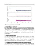
4.1 Scale spectra of global temperature records
The scale spectra of the global temperature data (CRUTEM3gl) display two extrema corre-
sponding to the existence of two cycles c
1
= 30 ± 3 months and c
2
= 43 ± 3 months. The
second cycle is also observed in the scale spectra of time series where the SST is taken into
account (HadCRUT3, HadCRUT3v, HadSST2 and GLB-T). The existence of c
1

in these data is
not so clear. The scale spectra of these series are shown in Fig. 4 and Fig. 5.
0.04
0.05
0.06
0.07
0.08
0.09
0.1
0.11
12 30 43
anomalies [K]
[months]
CRUTEM3gl
11 m
30.6 m41.8 m
0.02
0.03
0.04
0.05
0.06
0.07
0.08
12 30 43
[months]
HadSST2
10.1 m
30.6 m
41.8 m
Fig. 4. The scale spectra of global temperature records. Crutem3 (left panel) and HadSST2

(right panel).
0.02
0.03
0.04
0.05
0.06
0.07
0.08
12 30 43
anomalies [K]
[months]
HadCRUT3
10.1 m
30.6 m
41.8 m
0.02
0.03
0.04
0.05
0.06
0.07
0.08
0.09
12 30 43
[months]
GLB-T
10.8 m
29.6 m
41.8 m
Fig. 5. The scale spectra of global temperature records: HadCRUT3 (left panel) and GLB-T

(right panel).
When considering hemispheric data, c
1
and c
2
are still observed. The scale spectra of the
global temperature time series in the Northern Hemisphere display a maximum correspond-
ing to c
1
. This cycle is more clearly observed in the data where the SST is not taken into ac-
count (i.e. with CRUTEM3nh), while c
2
is more distinctly seen in the other time series (NH-T,
HadCrut3, HadSST2), as seen in Fig. 6 and Fig. 7. The spectra related to the Southern Hemi-
sphere still display a maximum corresponding to c
2
. For the CRU time series (HadCRUT3sh
and HadSST2sh), the observed cycle that is the closest to c
1
is about 25 months, while the
scale spectrum of the GISS data (SH-T) display a cycle c
1
as marked as the cycle c
2
. The scale
spectra of these series are shown in Fig. 8 and Fig. 9.
0.02
0.04
0.06
0.08

0.1
0.12
0.14
0.16
12 30 43
anomalies [K]
[months]
CRUTEM3nh
11.6 m
29.6 m
40.4 m
0.025
0.03
0.035
0.04
0.045
0.05
0.055
0.06
0.065
0.07
12 30 43
[months]
HadSST2 NH
12 m
28.6 m
41.9 m
Fig. 6. The scale spectra of Northern Hemisphere temperature records: Crutem3 (left panel)
and HadSST2 (right panel).
4.2 Scale spectra of local temperature records

In Nicolay et al. (2009), the scale spectra of a hundred near-surface air temperature time series
have been computed using GISS Surface Temperature Analysis data (only the most complete
data were chosen). The cycles detected in some weather stations are given by Fig. 10 and
Table 1 (the location, the amplitude of the cycles found and the associated class of climate
Multi-months cycles observed in climatic data 33
0
1
2
3
4
5
6
7
8
6 12 30
[months]
Fig. 3. The scale spectrum Λ of f . The abscissa (logarithmic scale) represent the months.
Let us remark that the scale spectra computed in this work do not take into account values
that are subject to border effects.
4. Results
4.1 Scale spectra of global temperature records
The scale spectra of the global temperature data (CRUTEM3gl) display two extrema corre-
sponding to the existence of two cycles c
1
= 30 ± 3 months and c
2
= 43 ± 3 months. The
second cycle is also observed in the scale spectra of time series where the SST is taken into
account (HadCRUT3, HadCRUT3v, HadSST2 and GLB-T). The existence of c
1

0.08
0.09
0.1
0.11
0.12
12 30 43
[months]
NH-T
11.6 m
29.6 m
41.8 m
Fig. 7. The scale spectra of Northern Hemisphere temperature records: HadCRUT3 (left panel)
and NH-T (right panel).
0.06
0.07
0.08
0.09
0.1
0.11
0.12
12 30 43
anomalies [K]
[months]
CRUTEM3sh
11.2 m
31.7 m
43.3 m
0.02
0.03
0.04

0.05
0.06
0.07
0.08
0.09
0.1
12 30 43
[months]
HadSST2 SH
10.8 m
24.9 m
43.3 m
Fig. 8. The scale spectra of Southern Hemisphere temperature records: CRUTEM3 (left panel)
and HadSST2 (right panel).
are also presented). These stations were selected in order to cover most of the typical climate
areas (see for Rudloff (1981) more details). As expected, the scale spectrum leads to a correct
estimation of the annual temperature amplitude (the difference between the mean tempera-
ture of the warmest and coldest months). The weather stations located in Europe and Siberia
are clearly affected by the cycle c
1
, while weather stations in areas such as California, Brazil,
Caribbean Sea and Hawaii are inﬂuenced by c
2
. The North American Weather stations time
series analysis shows the presence of both c
1
and c
2
. Roughly speaking, the temperature am-
plitudes induced by the cycles c

1
and c
2
represent about one tenth of the annual amplitude.
0.02
0.03
0.04
0.05
0.06
0.07
0.08
0.09
0.1
12 30 43
anomalies [K]
[months]
HadCRUT3 SH
10.8 m
24.9 m
43.3 m
0.03
0.04
0.05
0.06
0.07
0.08
0.09
12 30 43
[months]
SH-T

11.2 m
27.6 m 43.3 m
Fig. 9. The scale spectra of Southern Hemisphere temperature records: HadCRUT3 (left panel)
and SH-T (right panel).
Weather stations Lat. Long. Cycle (m) Cycle amp. An. amp. Classif.
Uccle (Belgium) 50.8
◦
N 4.3
◦
E 30.4 ± 2.7 0.4 K 15 K DO
Zaragoza (Spain) 41.6
◦
N 0.9
◦
W 28.4 ± 2.4 0.3 K 18 K BS
The Pas (Canada) 54.0
◦
N 101.1
◦
W 28.5 ± 2.6 0.6 K 38 K EC
44.8
± 2.4 0.8 K
Fairbanks (Alaska) 64.8
◦
N 147.9
◦
W 28.5 ± 2.5 0.8 K 40 K EC
40.4
± 2.5 0.8 K
Verhojansk (Siberia) 67.5

◦
N 133.4
◦
E 31.7 ± 2.5 0.8 K 64 K EC
Jakutsk (Siberia) 62.0
◦
N 129.7
◦
E 28.6 ± 2.4 0.8 K 60 K EC
San Francisco (California) 37.6
◦
N 122.4
◦
W 41.8 ± 2.7 0.3 K 8 K Cs
Lander (Wyoming) 42.8
◦
N 108.7
◦
W 41.8 ± 2.6 0.6 K 28 K DC
Manaus (Brazil) 3.1
◦
S 60.0
◦
W 43.3 ± 2.4 0.3 K 3 K Ar
Belo Horizonte (Brazil) 19.9
◦
S 43.9
◦
W 41.8 ± 2.4 0.5 K 4 K Aw
Tahiti (French Polynesia) 17.6

◦
S 149.6
◦
W 41.8 ± 2.5 0.2 K 3 K Ar
Lihue (Hawaii) 22.0
◦
N 159.3
◦
W 41.8 ± 2.5 0.3 K 4 K Ar
Colombo (Sri Lanka) 6.9
◦
N 79.9
◦
E 44.5 ± 2.6 0.2 K 2 K Ar
Minicoy (India) 8.3
◦
N 73.2
◦
E 41.8 ± 2.6 0.2 K 2 K Aw
Table 1. Cycles found in some world weather stations (the errors are estimated as in Nicolay
et al. (2009)). The stations were selected to represent the main climatic areas. For the class of
climates, see Rudloff (1981).
To show, that c
1
and c
2
affect the whole planet, the scale spectrum of each grid point of the
NCEP/NCAR reanalysis has been computed. As displayed in Fig. 11 and Fig. 12, 92% of the
Earth area is associated to at least one of these cycles. Fig. 11 shows that c
1

is mainly seen
in Alaska, Eastern Canada, Europe, Northern Asia and Turkey, while Fig. 12 reveals that c
2
is principally seen in Equatorial Paciﬁc, Northern America and Peru. Roughly speaking, the
cycle c
1
is observed in regions associated with the Arctic Oscillation, while c
2
is detected in
regions associated to the Southern Oscillation.
4.3 Scale spectra of atmospheric indices
Advection causes the transfer of air masses to neighboring regions, carrying their properties
such as air temperature. The climatic indices characterize these air mass movements.
Multi-months cycles observed in climatic data 35
0.03
0.035
0.04
0.045
0.05
0.055
0.06
0.065
0.07
0.075
0.08
0.085
12 30 43
anomalies [K]
[months]
HadCRUT3 NH

10.5 m
28.6 m
41.8 m
0.02
0.03
0.04
0.05
0.06
0.07
0.08
0.09
0.1
0.11
0.12
12 30 43
[months]
NH-T
11.6 m
29.6 m
41.8 m
Fig. 7. The scale spectra of Northern Hemisphere temperature records: HadCRUT3 (left panel)
and NH-T (right panel).
0.06
0.07
0.08
0.09
0.1
0.11
0.12
12 30 43

anomalies [K]
[months]
CRUTEM3sh
11.2 m
31.7 m
43.3 m
0.02
0.03
0.04
0.05
0.06
0.07
0.08
0.09
0.1
12 30 43
[months]
HadSST2 SH
10.8 m
24.9 m
43.3 m
Fig. 8. The scale spectra of Southern Hemisphere temperature records: CRUTEM3 (left panel)
and HadSST2 (right panel).
are also presented). These stations were selected in order to cover most of the typical climate
areas (see for Rudloff (1981) more details). As expected, the scale spectrum leads to a correct
estimation of the annual temperature amplitude (the difference between the mean tempera-
ture of the warmest and coldest months). The weather stations located in Europe and Siberia
are clearly affected by the cycle c
1
, while weather stations in areas such as California, Brazil,

Caribbean Sea and Hawaii are inﬂuenced by c
2
. The North American Weather stations time
series analysis shows the presence of both c
1
and c
2
. Roughly speaking, the temperature am-
plitudes induced by the cycles c
1
and c
2
represent about one tenth of the annual amplitude.
0.02
0.03
0.04
0.05
0.06
0.07
0.08
0.09
0.1
12 30 43
anomalies [K]
[months]
HadCRUT3 SH
10.8 m
24.9 m
43.3 m
0.03

0.04
0.05
0.06
0.07
0.08
0.09
12 30 43
[months]
SH-T
11.2 m
27.6 m 43.3 m
Fig. 9. The scale spectra of Southern Hemisphere temperature records: HadCRUT3 (left panel)
and SH-T (right panel).
Weather stations Lat. Long. Cycle (m) Cycle amp. An. amp. Classif.
Uccle (Belgium) 50.8
◦
N 4.3
◦
E 30.4 ± 2.7 0.4 K 15 K DO
Zaragoza (Spain) 41.6
◦
N 0.9
◦
W 28.4 ± 2.4 0.3 K 18 K BS
The Pas (Canada) 54.0
◦
N 101.1
◦
W 28.5 ± 2.6 0.6 K 38 K EC
44.8

± 2.4 0.8 K
Fairbanks (Alaska) 64.8
◦
N 147.9
◦
W 28.5 ± 2.5 0.8 K 40 K EC
40.4
± 2.5 0.8 K
Verhojansk (Siberia) 67.5
◦
N 133.4
◦
E 31.7 ± 2.5 0.8 K 64 K EC
Jakutsk (Siberia) 62.0
◦
N 129.7
◦
E 28.6 ± 2.4 0.8 K 60 K EC
San Francisco (California) 37.6
◦
N 122.4
◦
W 41.8 ± 2.7 0.3 K 8 K Cs
Lander (Wyoming) 42.8
◦
N 108.7
◦
W 41.8 ± 2.6 0.6 K 28 K DC
Manaus (Brazil) 3.1
◦

S 60.0
◦
W 43.3 ± 2.4 0.3 K 3 K Ar
Belo Horizonte (Brazil) 19.9
◦
S 43.9
◦
W 41.8 ± 2.4 0.5 K 4 K Aw
Tahiti (French Polynesia) 17.6
◦
S 149.6
◦
W 41.8 ± 2.5 0.2 K 3 K Ar
Lihue (Hawaii) 22.0
◦
N 159.3
◦
W 41.8 ± 2.5 0.3 K 4 K Ar
Colombo (Sri Lanka) 6.9
◦
N 79.9
◦
E 44.5 ± 2.6 0.2 K 2 K Ar
Minicoy (India) 8.3
◦
N 73.2
◦
E 41.8 ± 2.6 0.2 K 2 K Aw
Table 1. Cycles found in some world weather stations (the errors are estimated as in Nicolay
et al. (2009)). The stations were selected to represent the main climatic areas. For the class of

climates, see Rudloff (1981).
To show, that c
1
and c
2
affect the whole planet, the scale spectrum of each grid point of the
NCEP/NCAR reanalysis has been computed. As displayed in Fig. 11 and Fig. 12, 92% of the
Earth area is associated to at least one of these cycles. Fig. 11 shows that c
1
is mainly seen
in Alaska, Eastern Canada, Europe, Northern Asia and Turkey, while Fig. 12 reveals that c
2
is principally seen in Equatorial Paciﬁc, Northern America and Peru. Roughly speaking, the
cycle c
1
is observed in regions associated with the Arctic Oscillation, while c
2
is detected in
regions associated to the Southern Oscillation.
4.3 Scale spectra of atmospheric indices
Advection causes the transfer of air masses to neighboring regions, carrying their properties
such as air temperature. The climatic indices characterize these air mass movements.
Climate Change and Variability36
0.1
0.15
0.2
0.25
0.3
0.35
0.4

0.45
0.5
0.55
0.6
30 43 64
[K]
[months]
Uccle
30.4 m
0.45
0.5
0.55
0.6
0.65
0.7
0.75
0.8
30 43 64
[months]
The Pas
28.6 m
44.8 m
0.3
0.4
0.5
0.6
0.7
0.8
0.9
1

30 43 64
[K]
[months]
Verhojansk
31.7 m
0.2
0.22
0.24
0.26
0.28
0.3
0.32
0.34
0.36
0.38
0.4
30 43 64
[months]
San Francisco
41.9 m
0.12
0.14
0.16
0.18
0.2
0.22
0.24
0.26
0.28
0.3

30 43 64
[K]
[months]
Manaus
43.3 m
0.05
0.1
0.15
0.2
0.25
0.3
0.35
0.4
30 43 64
[months]
Lihue
41.8 m
Fig. 10. Scale spectra of near-surface air temperature time series: Uccle (Belgium), The Pas
(Canada), Verhojansk (Siberia), San Francisco (California), Manaus (Brazil), Lihue (Hawaii).
The cycles detected in the main climatic indices are reported in Table 2. Almost all these
indices display a cycle corresponding to c
1
, the notable exceptions being the NP, PNA and
global-SST ENSO indices. The cycle c
2
is observed in the AO (CPC), NP, PDO, PNA and SOI*
indices, as well as the indices related to the Southern Oscillation (such as the ENSO indices).
The scale spectra of these indices are shown in Fig. 13, 14, 15 and 16.
Fig. 11. NCEP/NCAR reanalysis data. The grid points where a cycle corresponding to c
1

has
been detected are coloured.
Fig. 12. NCEP/NCAR reanalysis data. The grid points where a cycle corresponding to c
2
has
been detected are coloured.
Index cycle c
1
cycle c
2
AO (CPC) 34 ± 2.6 43 ± 2.5
QBO 29
± 2
Global-SST ENSO 45
± 2.1
MEI ENSO 30
± 2.1 45 ± 2.1
NAO (CPC) 34
± 2.1
NAO (CRU) 34
± 2.1
NOI 32
± 2.3
NP 43
± 2.4
PDO 26
± 2.4 40 ± 2.3
PNA 45
± 2.4
SOI 30

± 2.2
SOI* 30
± 2.5 44 ± 2.6
Table 2. Cycles found in the main climatic indices (the errors are estimated as in Nicolay et al.
(2009)).
Multi-months cycles observed in climatic data 37
0.1
0.15
0.2
0.25
0.3
0.35
0.4
0.45
0.5
0.55
0.6
30 43 64
[K]
[months]
Uccle
30.4 m
0.45
0.5
0.55
0.6
0.65
0.7
0.75
0.8

30 43 64
[months]
The Pas
28.6 m
44.8 m
0.3
0.4
0.5
0.6
0.7
0.8
0.9
1
30 43 64
[K]
[months]
Verhojansk
31.7 m
0.2
0.22
0.24
0.26
0.28
0.3
0.32
0.34
0.36
0.38
0.4
30 43 64

[months]
San Francisco
41.9 m
0.12
0.14
0.16
0.18
0.2
0.22
0.24
0.26
0.28
0.3
30 43 64
[K]
[months]
Manaus
43.3 m
0.05
0.1
0.15
0.2
0.25
0.3
0.35
0.4
30 43 64
[months]
Lihue
41.8 m

Fig. 10. Scale spectra of near-surface air temperature time series: Uccle (Belgium), The Pas
(Canada), Verhojansk (Siberia), San Francisco (California), Manaus (Brazil), Lihue (Hawaii).
The cycles detected in the main climatic indices are reported in Table 2. Almost all these
indices display a cycle corresponding to c
1
, the notable exceptions being the NP, PNA and
global-SST ENSO indices. The cycle c
2
is observed in the AO (CPC), NP, PDO, PNA and SOI*
indices, as well as the indices related to the Southern Oscillation (such as the ENSO indices).
The scale spectra of these indices are shown in Fig. 13, 14, 15 and 16.
Fig. 11. NCEP/NCAR reanalysis data. The grid points where a cycle corresponding to c
1
has
been detected are coloured.
Fig. 12. NCEP/NCAR reanalysis data. The grid points where a cycle corresponding to c
2
has
been detected are coloured.
Index cycle c
1
cycle c
2
AO (CPC) 34 ± 2.6 43 ± 2.5
QBO 29
± 2
Global-SST ENSO 45
± 2.1
MEI ENSO 30
± 2.1 45 ± 2.1

NAO (CPC) 34
± 2.1
NAO (CRU) 34
± 2.1
NOI 32
± 2.3
NP 43
± 2.4
PDO 26
± 2.4 40 ± 2.3
PNA 45
± 2.4
SOI 30
± 2.2
SOI* 30
± 2.5 44 ± 2.6
Table 2. Cycles found in the main climatic indices (the errors are estimated as in Nicolay et al.
(2009)).
Climate Change and Variability38
0.05
0.1
0.15
0.2
0.25
0.3
0.35
0.4
0.45
0.5
12 30 43 64

[months]
AO (CPC)
12 m
34 m
43.3 m
5
10
15
20
25
30
35
40
45
50
12 30 43 64
[months]
NAM
12 m
34 m
0.1
0.15
0.2
0.25
0.3
0.35
0.4
12 30 43 64
[months]
NAO (CPC)

11 m
34 m
0.1
0.2
0.3
0.4
0.5
0.6
0.7
12 30 43 64
[months]
NAO (CRU)
9.75 m
24.9 m
34 m
Fig. 13. Scale spectra of the climatic indices related to the Northern Atlantic Oscillation.
4.4 A statistical validation for the observed cycles
Although many evidences attest the validity of the method described above, a question nat-
urally remains: Is there a high probability that the maxima observed in the scale spectra oc-
curred by pure chance?
In Nicolay et al. (2010), to check if the cycles observed in the time series can be trusted,
the scale spectra of the NCEP/NCAR reanalysis data have been compared with the spectra
of signals made of an autoregressive model of the ﬁrst order (AR(1) model, see e.g. Janacek
(2001)), in which maxima could occur fortuitously. Such processes are observed in many
climatic and geophysical data (see e.g. Allen & Robertson (1996); Percival & Walden (1993))
and are well suited for the study of climatic time series (see e.g. Mann & Lees (1996); Mann et
al. (2007)).
An artiﬁcial signal
(y
n

) can be associated to the temperature time series (x
n
) of a grid point of
the NCEP/NCAR reanalysis data as follows:
• One ﬁrst computes the climatological anomaly time series
(δ
n
) of (x
n
), i.e. for each
month, the mean temperature is calculated from the whole signal and the so-obtained
monthly-sampled signal
(m
n
) is subtracted to (x
n
), δ
n
= x
n
− m
n
.
• The anomaly time series
(δ
n
) is ﬁtted with an AR(1) model (
n
),


n
= α
n−1
+ ση
n
,
4
6
8
10
12
14
16
18
20
12 30 43 64
[months]
Global-SST ENSO
44.8 m
0.1
0.2
0.3
0.4
0.5
0.6
0.7
0.8
12 30 43 64
[months]
MEI ENSO

30.6 m
44.8 m
0.4
0.5
0.6
0.7
0.8
0.9
1
12 30 43 64
[months]
SOI
29.6 m
53.3 m
0.6
0.7
0.8
0.9
1
1.1
1.2
1.3
1.4
12 30 43 64
[months]
SOI*
9.1 m
29.6 m
44.8 m
0.7

0.8
0.9
1
1.1
1.2
1.3
12 30 43 64
[months]
NOI
10.5 m
19.5 m
31.7 m
55 m
0.1
0.15
0.2
0.25
0.3
0.35
0.4
0.45
0.5
12 30 43 64
[months]
PDO
11.6 m 25.7 m
40.4 m
Fig. 14. Scale spectra of the climatic indices related to the Southern Oscillation.
where η
n

is a Gaussian white noise with zero mean and unit variance (see e.g. Janacek
(2001)).
• The artiﬁcial signal
(y
n
) associated to (x
n
) is deﬁned by replacing (δ
n
) with (
n
), y
n
=
m
n
+ 
n
.
Let us remark that
(y
n
) is indeed a stochastic process; several simulations of the same signal
(x
n
) will thus yield different realizations.
Multi-months cycles observed in climatic data 39
0.05
0.1
0.15

0.2
0.25
0.3
0.35
0.4
0.45
0.5
12 30 43 64
[months]
AO (CPC)
12 m
34 m
43.3 m
5
10
15
20
25
30
35
40
45
50
12 30 43 64
[months]
NAM
12 m
34 m
0.1
0.15

0.2
0.25
0.3
0.35
0.4
12 30 43 64
[months]
NAO (CPC)
11 m
34 m
0.1
0.2
0.3
0.4
0.5
0.6
0.7
12 30 43 64
[months]
NAO (CRU)
9.75 m
24.9 m
34 m
Fig. 13. Scale spectra of the climatic indices related to the Northern Atlantic Oscillation.
4.4 A statistical validation for the observed cycles
Although many evidences attest the validity of the method described above, a question nat-
urally remains: Is there a high probability that the maxima observed in the scale spectra oc-
curred by pure chance?
In Nicolay et al. (2010), to check if the cycles observed in the time series can be trusted,
the scale spectra of the NCEP/NCAR reanalysis data have been compared with the spectra

of signals made of an autoregressive model of the ﬁrst order (AR(1) model, see e.g. Janacek
(2001)), in which maxima could occur fortuitously. Such processes are observed in many
climatic and geophysical data (see e.g. Allen & Robertson (1996); Percival & Walden (1993))
and are well suited for the study of climatic time series (see e.g. Mann & Lees (1996); Mann et
al. (2007)).
An artiﬁcial signal
(y
n
) can be associated to the temperature time series (x
n
) of a grid point of
the NCEP/NCAR reanalysis data as follows:
• One ﬁrst computes the climatological anomaly time series
(δ
n
) of (x
n
), i.e. for each
month, the mean temperature is calculated from the whole signal and the so-obtained
monthly-sampled signal
(m
n
) is subtracted to (x
n
), δ
n
= x
n
− m
n

.
• The anomaly time series
(δ
n
) is ﬁtted with an AR(1) model (
n
),

n
= α
n−1
+ ση
n
,
4
6
8
10
12
14
16
18
20
12 30 43 64
[months]
Global-SST ENSO
44.8 m
0.1
0.2
0.3

0.4
0.5
0.6
0.7
0.8
12 30 43 64
[months]
MEI ENSO
30.6 m
44.8 m
0.4
0.5
0.6
0.7
0.8
0.9
1
12 30 43 64
[months]
SOI
29.6 m
53.3 m
0.6
0.7
0.8
0.9
1
1.1
1.2
1.3

1.4
12 30 43 64
[months]
SOI*
9.1 m
29.6 m
44.8 m
0.7
0.8
0.9
1
1.1
1.2
1.3
12 30 43 64
[months]
NOI
10.5 m
19.5 m
31.7 m
55 m
0.1
0.15
0.2
0.25
0.3
0.35
0.4
0.45
0.5

12 30 43 64
[months]
PDO
11.6 m 25.7 m
40.4 m
Fig. 14. Scale spectra of the climatic indices related to the Southern Oscillation.
where η
n
is a Gaussian white noise with zero mean and unit variance (see e.g. Janacek
(2001)).
• The artiﬁcial signal
(y
n
) associated to (x
n
) is deﬁned by replacing (δ
n
) with (
n
), y
n
=
m
n
+ 
n
.
Let us remark that
(y
n

) is indeed a stochastic process; several simulations of the same signal
(x
n
) will thus yield different realizations.
Climate Change and Variability40
0.1
0.15
0.2
0.25
0.3
0.35
0.4
0.45
0.5
12 30 43 64
[months]
PNA (CPC)
11.2 m
19.5 m
29.6 m
44.8 m
5
10
15
20
25
30
35
40
45

12 30 43 64
[months]
PNA (JISAO)
10.1 m
18.2 m
44.4 m
Fig. 15. Scale spectra of the PNA indices.
0.2
0.3
0.4
0.5
0.6
0.7
0.8
0.9
1
1.1
1.2
30 43 64
[months]
NP
43.3 m
10
15
20
25
30
35
40
45

50
12 30 43 64
[months]
EOF3 (JISAO)
8.8 m
19.5 m
29.6 m
53.3 m
Fig. 16. Scale spectra of other climatic indices.
To check if the cycles c
1
and c
2
appearing in the time series did not occur by pure chance, the
subsequent methodology can be applied to each temperature time series
(x
n
) of the NCEP/NCAR
reanalysis data:
• N
= 10, 000 realizations (y
n
) of (x
n
) are computed.
• The distribution of the highest local maximum y
M
of the scale spectrum of the data in
the range of 26 to 47 months is estimated from these artiﬁcial signals, i.e. one computes
the distribution of

y
M
= sup
26≤a≤47
˜
Λ
(a),
where
˜
Λ is the scale spectrum of a realization
(y
n
).
• The probability P to obtain a maximum of higher amplitude than the one correspond-
ing to c
1
or c
2
observed in the scale spectrum of (x
n
) is ﬁnally computed, using the
distribution previously obtained.
It is shown in Nicolay et al. (2010) that such a methodology yields reliable data. The probabil-
ity values concerning c
1
and c
2
are displayed in Fig. 17 and Fig. 18 respectively. The coloured
area correspond to regions where the cycle is signiﬁcant. These ﬁgures show that most of the
cycles associated with c

1
and c
2
can be considered as signiﬁcant. The cycle observed in the cli-
matic indices are also signiﬁcant, since one always get P
< 0.1 (see Mabille & Nicolay (2009);
Nicolay et al. (2010)).
Finally, let us remark that c
1
and c
2
can also be detected through the Fourier transform, if the
time series are preprocessed in order to free the corresponding spectrum from the dominating
cycle corresponding to one year (for more details, see Nicolay et al. (2010)).
Fig. 17. The probability values associated with c
1
(NCEP/NCAR reanalysis data). The cycles
observed in a zone corresponding to the colour white are not signiﬁcant.
Fig. 18. The probability values associated with c
2
(NCEP/NCAR reanalysis data). The cycles
observed in a zone corresponding to the colour white are not signiﬁcant.
5. Discussion and conclusions
The wavelet-based tool introduced in Sect. 3.1 provides a methodology for detecting cycles in
non-stationary signals. Its application to climatic time series has led to the detection of two
statistically signiﬁcant periods of 30 and 43 months respectively.
When looking at the global temperature time series, since most of the lands are situated on the
Northern Hemisphere, the cycle c
1
seems to be inﬂuenced by the continents, while the cycle c

2
appears to be more inﬂuenced by the oceans. However, considering that only a small number
Multi-months cycles observed in climatic data 41
0.1
0.15
0.2
0.25
0.3
0.35
0.4
0.45
0.5
12 30 43 64
[months]
PNA (CPC)
11.2 m
19.5 m
29.6 m
44.8 m
5
10
15
20
25
30
35
40
45
12 30 43 64
[months]

PNA (JISAO)
10.1 m
18.2 m
44.4 m
Fig. 15. Scale spectra of the PNA indices.
0.2
0.3
0.4
0.5
0.6
0.7
0.8
0.9
1
1.1
1.2
30 43 64
[months]
NP
43.3 m
10
15
20
25
30
35
40
45
50
12 30 43 64

[months]
EOF3 (JISAO)
8.8 m
19.5 m
29.6 m
53.3 m
Fig. 16. Scale spectra of other climatic indices.
To check if the cycles c
1
and c
2
appearing in the time series did not occur by pure chance, the
subsequent methodology can be applied to each temperature time series
(x
n
) of the NCEP/NCAR
reanalysis data:
• N
= 10, 000 realizations (y
n
) of (x
n
) are computed.
• The distribution of the highest local maximum y
M
of the scale spectrum of the data in
the range of 26 to 47 months is estimated from these artiﬁcial signals, i.e. one computes
the distribution of
y
M

= sup
26≤a≤47
˜
Λ
(a),
where
˜
Λ is the scale spectrum of a realization
(y
n
).
• The probability P to obtain a maximum of higher amplitude than the one correspond-
ing to c
1
or c
2
observed in the scale spectrum of (x
n
) is ﬁnally computed, using the
distribution previously obtained.
It is shown in Nicolay et al. (2010) that such a methodology yields reliable data. The probabil-
ity values concerning c
1
and c
2
are displayed in Fig. 17 and Fig. 18 respectively. The coloured
area correspond to regions where the cycle is signiﬁcant. These ﬁgures show that most of the
cycles associated with c
1
and c

2
can be considered as signiﬁcant. The cycle observed in the cli-
matic indices are also signiﬁcant, since one always get P
< 0.1 (see Mabille & Nicolay (2009);
Nicolay et al. (2010)).
Finally, let us remark that c
1
and c
2
can also be detected through the Fourier transform, if the
time series are preprocessed in order to free the corresponding spectrum from the dominating
cycle corresponding to one year (for more details, see Nicolay et al. (2010)).
Fig. 17. The probability values associated with c
1
(NCEP/NCAR reanalysis data). The cycles
observed in a zone corresponding to the colour white are not signiﬁcant.
Fig. 18. The probability values associated with c
2
(NCEP/NCAR reanalysis data). The cycles
observed in a zone corresponding to the colour white are not signiﬁcant.
5. Discussion and conclusions
The wavelet-based tool introduced in Sect. 3.1 provides a methodology for detecting cycles in
non-stationary signals. Its application to climatic time series has led to the detection of two
statistically signiﬁcant periods of 30 and 43 months respectively.
When looking at the global temperature time series, since most of the lands are situated on the
Northern Hemisphere, the cycle c
1
seems to be inﬂuenced by the continents, while the cycle c
2
appears to be more inﬂuenced by the oceans. However, considering that only a small number

Climate Change and Variability Part 2 ppt

Tài liệu liên quan

Tài liệu bạn tìm kiếm đã sẵn sàng tải về