Climate Change and Variability Part 3 ppt

Climate Change and Variability48
satellite-based monthly precipitation product and a merged, short-record (1998-2006) 1
o
1
o

TRMM (3B43) monthly rainfall product (not shown). The basin-mean rainfall is computed
over a domain of 15
o
S-22.5
o
N, 15
o
-35
o
W. Finally, P
ITCZ
, Lat
ITCZ
, and P
dm
are determined by
subtracting their corresponding mean seasonal cycles.
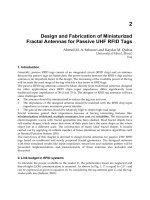
Time series for these three indices are depicted in Fig. 2. Rainfall changes during these two
seasons are comparable calibrated by either P
ITCZ
or P
dm
. However, the ITCZ does not
change much its mean latitudes during JJA, in contrast to evident fluctuations during MAM.

Thus the major rainfall changes during JJA are related to the variability of the ITCZ strength
and/or the basin-mean rainfall. This probably implies a lack of forcing mechanism on the
ITCZ location during JJA. Past studies suggested that the Atlantic interhemispheric SST
mode, though a dominant factor of the ITCZ position during MAM, becomes secondary
during JJA (e.g., Sutton et al., 2000; Gu & Adler, 2006).

Fig. 2. Time series of (a) the domain-mean rainfall (P
dm
), (b) the ITCZ strength (P
ITCZ
), and
(c) the ITCZ latitudes (Lat
ITCZ
) during JJA (solid) and MAM (dash-dot).

Simultaneous correlations between SST anomalies with P
ITCZ
and Lat
ITCZ
are estimated
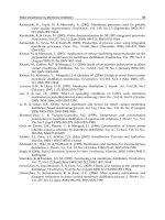
during both seasons (Fig. 3). During JJA, the major high-correlation area of SST anomalies
with P
ITCZ
is located west of about 120
o
W in the tropical central-eastern Pacific, and the
correlations between SST anomalies and Lat
ITCZ
are generally weak in the tropical Pacific.
Within the tropical Atlantic, significant, positive correlations with P

ITCZ
roughly cover the
entire basin from 20
o
S to 20
o
N. It is of interest to note that the same sign correlation is found
both north and south of the equator, suggesting a coherent, local forcing of rainfall
variability during JJA. Furthermore, evident negative correlations between SST anomalies
and Lat
ITCZ
are seen within the deep tropics especially along and south of the equator. These
confirm the weakening effect of the interhemispheric SST gradient mode during JJA (e.g.,
Sutton et al., 2000).
During MAM, the ITCZ strength is strongly correlated to SST anomalies in both the
equatorial Pacific and Atlantic (e.g., Nobre & Shukla, 1996; Sutton et al., 2000; Chiang et al.,
2002). However, the significant negative correlations tend to appear along the equator in the
central-eastern equatorial Pacific (east of 180
o
W) and along the western coast of South
America, quite different than during JJA. Roughly similar correlation patterns can also be
observed for Lat
ITCZ
in the tropical Pacific. Within the tropical Atlantic basin, P
ITCZ
tends to
be correlated with SST anomalies along and south of the equator, but the high correlation
area shrinks into a much smaller one compared with that during JJA. The lack of high
(negative) correlation north of the equator further confirms that the interhemispheric SST
mode strongly impacts the ITCZ locations (Fig. 3d), but has a minor effect on the ITCZ

strength (e.g., Nobre & Shukla, 1996).


Fig. 3. Correlations of SST anomalies with (a, c) the ITCZ strength (P
ITCZ
) and (b, d) the ITCZ
latitude (Lat
ITCZ
) during (a, b) MAM and (c, d) JJA. The 5% significance level is 0.4 based on
23 degrees of freedom (dofs).

During these two seasons there are also two major large areas of high correlation for both
P
ITCZ
and Lat
ITCZ
in the tropical western Pacific, though with different spatial features: One
is along the South Pacific Convergence Zone (SPCZ), another is north of 10
o
N. These two
features are probably associated with the ENSO effect and other factors, and not directly
related to the changes in the tropical Atlantic, which are supported by weak regressed SST
anomalies (not shown).
Summer-Time Rainfall Variability in the Tropical Atlantic 49
satellite-based monthly precipitation product and a merged, short-record (1998-2006) 1
o
1
o

TRMM (3B43) monthly rainfall product (not shown). The basin-mean rainfall is computed

over a domain of 15
o
S-22.5
o
N, 15
o
-35
o
W. Finally, P
ITCZ
, Lat
ITCZ
, and P
dm
are determined by
subtracting their corresponding mean seasonal cycles.
Time series for these three indices are depicted in Fig. 2. Rainfall changes during these two
seasons are comparable calibrated by either P
ITCZ
or P
dm
. However, the ITCZ does not
change much its mean latitudes during JJA, in contrast to evident fluctuations during MAM.
Thus the major rainfall changes during JJA are related to the variability of the ITCZ strength
and/or the basin-mean rainfall. This probably implies a lack of forcing mechanism on the
ITCZ location during JJA. Past studies suggested that the Atlantic interhemispheric SST
mode, though a dominant factor of the ITCZ position during MAM, becomes secondary
during JJA (e.g., Sutton et al., 2000; Gu & Adler, 2006).

Fig. 2. Time series of (a) the domain-mean rainfall (P

dm
), (b) the ITCZ strength (P
ITCZ
), and
(c) the ITCZ latitudes (Lat
ITCZ
) during JJA (solid) and MAM (dash-dot).

Simultaneous correlations between SST anomalies with P
ITCZ
and Lat
ITCZ
are estimated
during both seasons (Fig. 3). During JJA, the major high-correlation area of SST anomalies
with P
ITCZ
is located west of about 120
o
W in the tropical central-eastern Pacific, and the
correlations between SST anomalies and Lat
ITCZ
are generally weak in the tropical Pacific.
Within the tropical Atlantic, significant, positive correlations with P
ITCZ
roughly cover the
entire basin from 20
o
S to 20
o
N. It is of interest to note that the same sign correlation is found

both north and south of the equator, suggesting a coherent, local forcing of rainfall
variability during JJA. Furthermore, evident negative correlations between SST anomalies
and Lat
ITCZ
are seen within the deep tropics especially along and south of the equator. These
confirm the weakening effect of the interhemispheric SST gradient mode during JJA (e.g.,
Sutton et al., 2000).
During MAM, the ITCZ strength is strongly correlated to SST anomalies in both the
equatorial Pacific and Atlantic (e.g., Nobre & Shukla, 1996; Sutton et al., 2000; Chiang et al.,
2002). However, the significant negative correlations tend to appear along the equator in the
central-eastern equatorial Pacific (east of 180
o
W) and along the western coast of South
America, quite different than during JJA. Roughly similar correlation patterns can also be
observed for Lat
ITCZ
in the tropical Pacific. Within the tropical Atlantic basin, P
ITCZ
tends to
be correlated with SST anomalies along and south of the equator, but the high correlation
area shrinks into a much smaller one compared with that during JJA. The lack of high
(negative) correlation north of the equator further confirms that the interhemispheric SST
mode strongly impacts the ITCZ locations (Fig. 3d), but has a minor effect on the ITCZ
strength (e.g., Nobre & Shukla, 1996).


Fig. 3. Correlations of SST anomalies with (a, c) the ITCZ strength (P
ITCZ
) and (b, d) the ITCZ
latitude (Lat

ITCZ
) during (a, b) MAM and (c, d) JJA. The 5% significance level is 0.4 based on
23 degrees of freedom (dofs).

During these two seasons there are also two major large areas of high correlation for both
P
ITCZ
and Lat
ITCZ
in the tropical western Pacific, though with different spatial features: One
is along the South Pacific Convergence Zone (SPCZ), another is north of 10
o
N. These two
features are probably associated with the ENSO effect and other factors, and not directly
related to the changes in the tropical Atlantic, which are supported by weak regressed SST
anomalies (not shown).
Climate Change and Variability50
4. The effects of three major SST modes
To further explore the relationships between rainfall anomalies in the tropical Atlantic and
SST variability, particularly during JJA, three major SST indices are constructed. Here,
Nino3.4, the mean SST anomalies within a domain of 5
o
S-5
o
N, 120
o
-170
o
W, is as usual used
to denote the interannual variability in the tropical Pacific. As in Gu & Adler (2006), the SST

anomalies within 3
o
S-3
o
N, 0-20
o
W are defined as Atl3 to represent the Atlantic Equatorial
Oscillation (e.g., Zebiak, 1993; Carton & Huang, 1994). SST variability in the tropical north
Atlantic is denoted by SST anomalies averaged within a domain of 5
o
-25
o
N, 15
o
-55
o
W
(TNA). In addition, another index (TNA1) is constructed for comparison by SST anomalies
averaged over a slightly smaller domain, 5
o
-20
o
N, 15
o
-55
o
W. We are not going to focus on
the interhemispheric SST mode here because during boreal summer this mode becomes
weak and does not impact much on the ITCZ (e.g., Sutton et al., 2000; Gu & Adler, 2006), and
the evident variability of the ITCZ is its strength rather than its preferred latitudes (Fig. 2).

Same procedures are applied to surface zonal winds in the western basin (5
o
S-5
o
N, 25
o
-
45
o
W) to construct a surface zonal wind index (U
WAtl
).
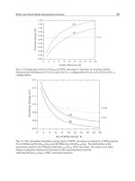
As discovered in past studies (e.g., Nobre & Shukla, 1996; Czaja, 2004), evident seasonal
preferences exist in these indices (Fig. 4). ENSO usually peaks during boreal winter. The
most intense variability in the tropical Atlantic appears during boreal spring and early
summer. The maxima of both TNA and TNA1 are in April, about three months later than
the strongest ENSO signals (e.g., Curtis & Hastenrath, 1995; Nobre & Shukla, 1996). Surface
zonal wind anomaly in the western equatorial region (U
WAtl
) attains its maximum in May,
followed by the most intense equatorial SST oscillation (Atl3) in June. Münnich & Neelin
(2005) suggested that there seems a chain reaction during this time period in the equatorial
Atlantic region. It is thus further arguable that the tropical western Atlantic (west of 20
o
W)
is a critical region passing and/or inducing climatic anomalies in the equatorial Atlantic
basin.

Fig. 4. Variances of various indices as a function of month. The variance of Nino 3.4 is scaled
by 2.

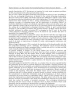
Fig. 5. Correlation coefficients between various indices as function of month. The 5%
significance level is 0.41 based on 21 dofs.

4.1 Relationships between various indices
Simultaneous correlations between SST indices are computed for each month (Fig. 5). The
Pacific Niño shows strong impact on the tropical Atlantic indices. Significant correlations
are found between Nino3.4 and TNA during February-April with a peak in March. The
negative correlation between Nino3.4 and Atl3 becomes statistically significant during
April-June, showing the impact of the ENSO on the Atlantic equatorial mode (e.g., Delecluse
et al., 1994; Latif & Grötzner, 2000). U
WAtl
is consistently, negatively correlated with Nino3.4
during April-July except in June when the correlation coefficient is slightly lower than the
5% significance level. Interestingly, there are two peak months (April and July) for the
correlation between U
WAtl
and Nino3.4 as discovered in Münnich & Neelin (2005). High
correlations between Atl3 and U
WAtl
occur during March-July. These correlation relations
tend to support that zonal wind anomalies at the surface in the western basin is a critical
part of the connection between the equatorial Pacific and the equatorial Atlantic. Münnich &
Neelin (2005) even showed a slightly stronger correlation relationship. Atl3 is also
significantly correlated to U
WAtl
in other several months, i.e., January, September, and
November, probably corresponding to the occasional appearance of the equatorial
oscillation event during boreal fall and winter (e.g., Wang, 2002; Gu & Adler, 2006).
Within the tropical Atlantic basin, the correlations between Atl3 and SST anomalies north of

the equator (TNA and TNA1) become positive and strong during late boreal summer,
particularly between Atl3 and TNA1 (above the 5% significance level during August-
October). As shown in Fig. 4, SST variations north of the equator become weaker during
boreal summer. Simultaneously the ITCZ and associated trade wind system move further to
the north. It thus seems possible to feel impact in the TNA/TNA1 region from the equatorial
region during this time period for surface wind anomalies-driven ocean transport (e.g., Gill,
1982).
Summer-Time Rainfall Variability in the Tropical Atlantic 51
4. The effects of three major SST modes
To further explore the relationships between rainfall anomalies in the tropical Atlantic and
SST variability, particularly during JJA, three major SST indices are constructed. Here,
Nino3.4, the mean SST anomalies within a domain of 5
o
S-5
o
N, 120
o
-170
o
W, is as usual used
to denote the interannual variability in the tropical Pacific. As in Gu & Adler (2006), the SST
anomalies within 3
o
S-3
o
N, 0-20
o
W are defined as Atl3 to represent the Atlantic Equatorial
Oscillation (e.g., Zebiak, 1993; Carton & Huang, 1994). SST variability in the tropical north
Atlantic is denoted by SST anomalies averaged within a domain of 5

o
-25
o
N, 15
o
-55
o
W
(TNA). In addition, another index (TNA1) is constructed for comparison by SST anomalies
averaged over a slightly smaller domain, 5
o
-20
o
N, 15
o
-55
o
W. We are not going to focus on
the interhemispheric SST mode here because during boreal summer this mode becomes
weak and does not impact much on the ITCZ (e.g., Sutton et al., 2000; Gu & Adler, 2006), and
the evident variability of the ITCZ is its strength rather than its preferred latitudes (Fig. 2).
Same procedures are applied to surface zonal winds in the western basin (5
o
S-5
o
N, 25
o
-
45
o

W) to construct a surface zonal wind index (U
WAtl
).
As discovered in past studies (e.g., Nobre & Shukla, 1996; Czaja, 2004), evident seasonal
preferences exist in these indices (Fig. 4). ENSO usually peaks during boreal winter. The
most intense variability in the tropical Atlantic appears during boreal spring and early
summer. The maxima of both TNA and TNA1 are in April, about three months later than
the strongest ENSO signals (e.g., Curtis & Hastenrath, 1995; Nobre & Shukla, 1996). Surface
zonal wind anomaly in the western equatorial region (U
WAtl
) attains its maximum in May,
followed by the most intense equatorial SST oscillation (Atl3) in June. Münnich & Neelin
(2005) suggested that there seems a chain reaction during this time period in the equatorial
Atlantic region. It is thus further arguable that the tropical western Atlantic (west of 20
o
W)
is a critical region passing and/or inducing climatic anomalies in the equatorial Atlantic
basin.

Fig. 4. Variances of various indices as a function of month. The variance of Nino 3.4 is scaled
by 2.

Fig. 5. Correlation coefficients between various indices as function of month. The 5%
significance level is 0.41 based on 21 dofs.

4.1 Relationships between various indices
Simultaneous correlations between SST indices are computed for each month (Fig. 5). The
Pacific Niño shows strong impact on the tropical Atlantic indices. Significant correlations
are found between Nino3.4 and TNA during February-April with a peak in March. The
negative correlation between Nino3.4 and Atl3 becomes statistically significant during

April-June, showing the impact of the ENSO on the Atlantic equatorial mode (e.g., Delecluse
et al., 1994; Latif & Grötzner, 2000). U
WAtl
is consistently, negatively correlated with Nino3.4
during April-July except in June when the correlation coefficient is slightly lower than the
5% significance level. Interestingly, there are two peak months (April and July) for the
correlation between U
WAtl
and Nino3.4 as discovered in Münnich & Neelin (2005). High
correlations between Atl3 and U
WAtl
occur during March-July. These correlation relations
tend to support that zonal wind anomalies at the surface in the western basin is a critical
part of the connection between the equatorial Pacific and the equatorial Atlantic. Münnich &
Neelin (2005) even showed a slightly stronger correlation relationship. Atl3 is also
significantly correlated to U
WAtl
in other several months, i.e., January, September, and
November, probably corresponding to the occasional appearance of the equatorial
oscillation event during boreal fall and winter (e.g., Wang, 2002; Gu & Adler, 2006).
Within the tropical Atlantic basin, the correlations between Atl3 and SST anomalies north of
the equator (TNA and TNA1) become positive and strong during late boreal summer,
particularly between Atl3 and TNA1 (above the 5% significance level during August-
October). As shown in Fig. 4, SST variations north of the equator become weaker during
boreal summer. Simultaneously the ITCZ and associated trade wind system move further to
the north. It thus seems possible to feel impact in the TNA/TNA1 region from the equatorial
region during this time period for surface wind anomalies-driven ocean transport (e.g., Gill,
1982).
Climate Change and Variability52
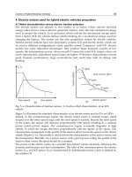
Lag-correlations between various SST indices are estimated to further our understanding of

the likely, casual relationships among them (Figs. 6, 7, and 8). The base months for SST
indices are chosen according to their respective peak months of variances (Fig. 4). The
strongest correlation between Atl3 in June and Nino3.4 is found when Nino3.4 leads Atl3 by
one month (Fig. 6), further confirming the remote forcing of ENSO on the Atlantic equatorial
mode (e.g., Latif & Grötzner, 2000). The 1-3 month leading, significant correlation of U
WAtl
to
Atl3 in June with a peak at one-month leading indicates that the equatorial oscillation is
mostly excited by surface zonal wind anomalies in the western basin likely through oceanic
dynamics (e.g., Zebiak, 1993; Carton & Huang, 1994; Delecluse et al., 1994; Latif & Grötzner,
2000).

Fig. 6. Lag-correlations between Atl3 in June with Nino3.4 and U
WAtl
, respectively. Positive
(negative) months indicate Atl3 leads (lags) Nino3.4 and U
WAtl
. The 5% significance level is
0.42 based on 20 dofs.

The lag-correlation between U
WAtl
in May and Nino3.4 is depicted in Fig. 7. The highest
correlation appears as Nino3.4 leads U
WAtl
by one-month, suggesting a strong impact from
the equatorial Pacific (e.g., Latif & Grötzner, 2000), and this impact probably being through
anomalous Walker circulation and not passing through the mid-latitudes.
North of the equator, TNA and TNA1 both peak in April (Fig. 4). Simultaneous correlations
between these two and Nino3.4 at the peak month are much weaker than when Nino3.4

leads them by at least one-month (Fig. 8). It is further noticed that the consistent high lag-
correlations are seen with Nino3.4 leading by 1-7 months. Significant correlations of TNA
and TNA1 in April with Nino3.4 can actually be found as Nino3.4 leads them up to 10
months (not shown). These highly consistent lag-relations suggest that the impact from the
equatorial Pacific on the tropical north Atlantic may go through two ways: the Pacific-
North-American (PNA) teleconnection and the anomalous Walker circulation (e.g., Nobre &
Shukla, 1996; Saravanan & Chang, 2000; Chiang et al., 2002), with the trade wind anomalies
being the critical means. Most previous studies generally emphasized the first means being
av
19
9

Fi
g
in
d

Fi
g
m
o
o
n
4.
2
T
a
T
N
ef

f
ailable durin
g
b
o
9
6).
g
. 7. Lag-correla
d
icate U
WAtl
lead
s
g
. 8. Lag-correlat
i
o
nths indicate T
N
n
20 dofs.

2
Spatial struct
u
a
bles 1 and 2 illu
s
N

A, and Nino3.
4
f
ectivel
y
impact
o
real winter and
tion between U
W
s
(la
g
s) Nino3.4.
T
i
ons between T
N
N
A and TNA1 le
a
u
res of three SS
T
s
trate the simult
a
4
) and two rain
f

rainfall variabili
t
sprin
g
(e.g., Cur
t
W
Atl
in Ma
y
wit
h
T
he 5% si
g
nifica
n
N
A and TNA1 in

a
d (la
g
) Nino3.4.

T
modes relate
d
a
neous correlati

o
f
all indices (P
IT
C
ty
in the tropic
a
t
is & Hastenrath,

h
Nino3.4. Posi
t
n
ce level is 0.42
b

April with Nin
o

The 5% si
g
nifica
variations
o
ns between the
t
C
Z

and Lat
ITCZ
).
T
a
l Atlantic (e.g.,
N

1995; Nobre &
S

t
ive (ne
g
ative)
m
b
ased on 20 dofs.

o
3.4. Positive (ne
g
nce level is 0.4
2
t
hree SST indice
s
T
he ENSO eve
n

N
obre & Shukla
,
S
hukla,
m
onths

g
ative)
2
based
s
(Atl3,
n
ts can
,
1996;
Summer-Time Rainfall Variability in the Tropical Atlantic 53
Lag-correlations between various SST indices are estimated to further our understanding of
the likely, casual relationships among them (Figs. 6, 7, and 8). The base months for SST
indices are chosen according to their respective peak months of variances (Fig. 4). The
strongest correlation between Atl3 in June and Nino3.4 is found when Nino3.4 leads Atl3 by
one month (Fig. 6), further confirming the remote forcing of ENSO on the Atlantic equatorial
mode (e.g., Latif & Grötzner, 2000). The 1-3 month leading, significant correlation of U
WAtl
to
Atl3 in June with a peak at one-month leading indicates that the equatorial oscillation is
mostly excited by surface zonal wind anomalies in the western basin likely through oceanic
dynamics (e.g., Zebiak, 1993; Carton & Huang, 1994; Delecluse et al., 1994; Latif & Grötzner,

2000).

Fig. 6. Lag-correlations between Atl3 in June with Nino3.4 and U
WAtl
, respectively. Positive
(negative) months indicate Atl3 leads (lags) Nino3.4 and U
WAtl
. The 5% significance level is
0.42 based on 20 dofs.

The lag-correlation between U
WAtl
in May and Nino3.4 is depicted in Fig. 7. The highest
correlation appears as Nino3.4 leads U
WAtl
by one-month, suggesting a strong impact from
the equatorial Pacific (e.g., Latif & Grötzner, 2000), and this impact probably being through
anomalous Walker circulation and not passing through the mid-latitudes.
North of the equator, TNA and TNA1 both peak in April (Fig. 4). Simultaneous correlations
between these two and Nino3.4 at the peak month are much weaker than when Nino3.4
leads them by at least one-month (Fig. 8). It is further noticed that the consistent high lag-
correlations are seen with Nino3.4 leading by 1-7 months. Significant correlations of TNA
and TNA1 in April with Nino3.4 can actually be found as Nino3.4 leads them up to 10
months (not shown). These highly consistent lag-relations suggest that the impact from the
equatorial Pacific on the tropical north Atlantic may go through two ways: the Pacific-
North-American (PNA) teleconnection and the anomalous Walker circulation (e.g., Nobre &
Shukla, 1996; Saravanan & Chang, 2000; Chiang et al., 2002), with the trade wind anomalies
being the critical means. Most previous studies generally emphasized the first means being
av
19

9

Fi
g
in
d

Fi
g
m
o
o
n
4.
2
T
a
T
N
ef
f
ailable durin
g
b
o
9
6).
g
. 7. Lag-correla
d

icate U
WAtl
lead
s
g
. 8. Lag-correlat
i
o
nths indicate T
N
n
20 dofs.

2
Spatial struct
u
a
bles 1 and 2 illu
s
N
A, and Nino3.
4
f
ectivel
y
impact
o
real winter and
tion between U
W

s
(la
g
s) Nino3.4.
T
i
ons between T
N
N
A and TNA1 le
a
u
res of three SS
T
s
trate the simult
a
4
) and two rain
f
rainfall variabili
t
sprin
g
(e.g., Cur
t
W
Atl
in Ma
y

wit
h
T
he 5% si
g
nifica
n
N
A and TNA1 in

a
d (la
g
) Nino3.4.

T
modes relate
d
a
neous correlati
o
f
all indices (P
IT
C
ty
in the tropic
a
t
is & Hastenrath,

h
Nino3.4. Posi
t
n
ce level is 0.42
b

April with Nin
o

The 5% si
g
nifica
variations
o
ns between the
t
C
Z
and Lat
ITCZ
).
T
a
l Atlantic (e.g.,
N

1995; Nobre &
S

t
ive (ne
g
ative)
m
b
ased on 20 dofs.

o
3.4. Positive (ne
g
nce level is 0.4
2
t
hree SST indice
s
T
he ENSO eve
n
N
obre & Shukla
,
S
hukla,
m
onths

g
ative)

2
based
s
(Atl3,
n
ts can
,
1996;
Climate Change and Variability54
Enfield & Mayer, 1997; Saravanan & Chang, 2000; Chiang et al., 2002; Giannini et al., 2004).
A higher correlation (-0.62) can even be obtained between Nino3.4 and P
dm
, implying a
basin-wide impact in the equatorial region. The correlation between Nino3.4 and Lat
ITCZ
is
relatively weak during JJA, in contrasting to a much stronger impact during MAM.
Significant correlations appear between Atl3, and P
ITCZ
and Lat
ITCZ
during JJA and MAM
(Tables 1 & 2). Even though the Atlantic equatorial warm/cold events are relatively weak
and the ITCZ tends to be located about eight degrees north of the equator during boreal
summer, the results suggest that the Atlantic Niño mode could still be a major factor
controlling the ITCZ strength.
For the effect of TNA, large seasonal differences exist in its correlations with the rainfall
indices (Tables 1 & 2). During JJA, TNA is significantly correlated with P
ITCZ
. During MAM,

however this correlation is much weaker. The correlation coefficient even changes sign
between these two seasons. On the other hand, TNA is significantly correlated to Lat
ITCZ

during MAM, but not during JJA.


Nino3.4 Atl3 TNA
P
ITCZ

-0.51 0.68 0.51
Lat
ITCZ
0.39
-0.65
0.04
Table 1. Correlation coefficients () between P
ITCZ
(mm day
-1
) and Lat
ITCZ
(degree), and
various SST indices during JJA. =0.40 is the 5% significance level based on (n-2=) 23 dofs.


Nino3.4 Atl3 TNA
P
ITCZ

-0.50 0.56
-0.18
Lat
ITCZ

0.57 -0.67 0.41
Table 2 Correlation coefficients () between P
ITCZ
(mm day
-1
) and Lat
ITCZ
(degree), and three
SST indices during MAM. =0.40 is the 5% significance level based on (n-2=) 23 dofs.

The modulations of the three major SST modes on the tropical Atlantic during JJA and
MAM are further quantified by computing the regressions based on their seasonal-mean
magnitudes normalized by their corresponding standard deviations.
Fig. 9 depicts the SST, surface wind, and precipitation associated with Atl3. During JJA, the
spatial patterns generally agree with shown in previous studies that primarily focused on
the peak months of the Atlantic equatorial mode (e.g., Ruiz-Barradas et al., 2000; Wang,
2002). Basin-wide warming is seen with the maximum SSTs along the equator and tends to
be in the eastern basin (Fig. 9b). Surface wind anomalies in general converge into the
maximum, positive SST anomaly zone. Accompanying strong cross-equatorial flows being
in the eastern equatorial region, anomalous westerlies are seen in the western basin
extending from the equator to about 15
o
N. These wind anomalies are related to the
equatorial warming (Figs. 5, 6), and also might be the major reason for the warming-up in

the TNA/TNA1 region. Off the coast of West Africa, there even exist weak southerly
anomalies between 10
o
-15
o
N. Positive rainfall anomalies are dominant in the entire basin,
corresponding to the warm SSTs. It is interesting to note that these rainfall anomalies tend to
be over the same area as the seasonal mean rainfall variances (Fig. 1). Particularly, over the
open ocean the maximum rainfall anomaly band is roughly sandwiched by the marine ITCZ
and the equatorial zone with maximum SST variability (Figs. 1c, 9b, and 9d), confirming the
strong modulations of the equatorial mode during this season (Fig. 2). During MAM,
positive SST anomalies already appear along the equator (Fig. 9a). However, in addition to
the SST anomalies along the equator, the most intense SST variability occurs right off the
west coast of Central Africa, reflecting the frequent appearance of the Benguela Niño
peaking in March-April (e.g., Florenchie et al., 2004). North of the equator, negative SST
anomalies, though very weak, can still be seen off the West African coast. This suggests that
the Atlantic Niño may effectively contribute to the interhemispheric SST mode peaking in
this season, particularly to its south lobe (Figs. 1b and 9a). Negative-positive rainfall
anomalies across the equator forming a dipolar structure are evident, specifically west of
20
o
W (Fig. 9c). In the Gulf of Guinea, positive rainfall anomalies, though much weaker than
in the western basin, can still be observed extending from the open ocean to the west coast
of Central Africa, roughly following strong positive SST anomalies.


Fig. 9. Regression onto Nino3.4 of SST and surface wind (a, b), and precipitation (c, d)
anomalies during JJA (a, c) and MAM (b, d).

The SST, surface wind, and rainfall anomalies associated with TNA are shown in Fig. 10.

Positive SST anomalies appear north of the equator during MAM, but become weaker
during JJA. Surface wind vectors converge into the warm SST region, resulting in the
decrease in the mean trade winds north of the equator. Cross-equatorial flow is strong
during MAM, implying TNA's contribution to the interhemispheric SST mode. On the other
hand, no evident SST anomalies appear along and south of the equator supporting that the
two lobes of the interhemispheric mode are probably not connected (e.g., Enfield et al.,
1999). A negative-positive rainfall dipolar feature occurs during MAM with much weaker
anomalies east of 20
o
W, consistent with previous studies (e.g., Nobre & Shukla, 1996; Ruiz-
Barradas et al., 2000; Chiang et al., 2002). During JJA, however only appears a single band of
positive rainfall anomalies between 5
o
-20
o
N, covering the northern portion of the mean
rainfall within the ITCZ and its variances (Figs. 1c, 1d, and 10d). Interestingly this band tilts
Summer-Time Rainfall Variability in the Tropical Atlantic 55
Enfield & Mayer, 1997; Saravanan & Chang, 2000; Chiang et al., 2002; Giannini et al., 2004).
A higher correlation (-0.62) can even be obtained between Nino3.4 and P
dm
, implying a
basin-wide impact in the equatorial region. The correlation between Nino3.4 and Lat
ITCZ
is
relatively weak during JJA, in contrasting to a much stronger impact during MAM.
Significant correlations appear between Atl3, and P
ITCZ
and Lat
ITCZ

during JJA and MAM
(Tables 1 & 2). Even though the Atlantic equatorial warm/cold events are relatively weak
and the ITCZ tends to be located about eight degrees north of the equator during boreal
summer, the results suggest that the Atlantic Niño mode could still be a major factor
controlling the ITCZ strength.
For the effect of TNA, large seasonal differences exist in its correlations with the rainfall
indices (Tables 1 & 2). During JJA, TNA is significantly correlated with P
ITCZ
. During MAM,
however this correlation is much weaker. The correlation coefficient even changes sign
between these two seasons. On the other hand, TNA is significantly correlated to Lat
ITCZ

during MAM, but not during JJA.



Nino3.4 Atl3 TNA
P
ITCZ

-0.51 0.68 0.51
Lat
ITCZ
0.39
-0.65
0.04
Table 1. Correlation coefficients () between P
ITCZ
(mm day

-1
) and Lat
ITCZ
(degree), and
various SST indices during JJA. =0.40 is the 5% significance level based on (n-2=) 23 dofs.



Nino3.4 Atl3 TNA
P
ITCZ

-0.50 0.56
-0.18
Lat
ITCZ

0.57 -0.67 0.41
Table 2 Correlation coefficients () between P
ITCZ
(mm day
-1
) and Lat
ITCZ
(degree), and three
SST indices during MAM. =0.40 is the 5% significance level based on (n-2=) 23 dofs.

The modulations of the three major SST modes on the tropical Atlantic during JJA and
MAM are further quantified by computing the regressions based on their seasonal-mean
magnitudes normalized by their corresponding standard deviations.

Fig. 9 depicts the SST, surface wind, and precipitation associated with Atl3. During JJA, the
spatial patterns generally agree with shown in previous studies that primarily focused on
the peak months of the Atlantic equatorial mode (e.g., Ruiz-Barradas et al., 2000; Wang,
2002). Basin-wide warming is seen with the maximum SSTs along the equator and tends to
be in the eastern basin (Fig. 9b). Surface wind anomalies in general converge into the
maximum, positive SST anomaly zone. Accompanying strong cross-equatorial flows being
in the eastern equatorial region, anomalous westerlies are seen in the western basin
extending from the equator to about 15
o
N. These wind anomalies are related to the
equatorial warming (Figs. 5, 6), and also might be the major reason for the warming-up in
the TNA/TNA1 region. Off the coast of West Africa, there even exist weak southerly
anomalies between 10
o
-15
o
N. Positive rainfall anomalies are dominant in the entire basin,
corresponding to the warm SSTs. It is interesting to note that these rainfall anomalies tend to
be over the same area as the seasonal mean rainfall variances (Fig. 1). Particularly, over the
open ocean the maximum rainfall anomaly band is roughly sandwiched by the marine ITCZ
and the equatorial zone with maximum SST variability (Figs. 1c, 9b, and 9d), confirming the
strong modulations of the equatorial mode during this season (Fig. 2). During MAM,
positive SST anomalies already appear along the equator (Fig. 9a). However, in addition to
the SST anomalies along the equator, the most intense SST variability occurs right off the
west coast of Central Africa, reflecting the frequent appearance of the Benguela Niño
peaking in March-April (e.g., Florenchie et al., 2004). North of the equator, negative SST
anomalies, though very weak, can still be seen off the West African coast. This suggests that
the Atlantic Niño may effectively contribute to the interhemispheric SST mode peaking in
this season, particularly to its south lobe (Figs. 1b and 9a). Negative-positive rainfall
anomalies across the equator forming a dipolar structure are evident, specifically west of

20
o
W (Fig. 9c). In the Gulf of Guinea, positive rainfall anomalies, though much weaker than
in the western basin, can still be observed extending from the open ocean to the west coast
of Central Africa, roughly following strong positive SST anomalies.


Fig. 9. Regression onto Nino3.4 of SST and surface wind (a, b), and precipitation (c, d)
anomalies during JJA (a, c) and MAM (b, d).

The SST, surface wind, and rainfall anomalies associated with TNA are shown in Fig. 10.
Positive SST anomalies appear north of the equator during MAM, but become weaker
during JJA. Surface wind vectors converge into the warm SST region, resulting in the
decrease in the mean trade winds north of the equator. Cross-equatorial flow is strong
during MAM, implying TNA's contribution to the interhemispheric SST mode. On the other
hand, no evident SST anomalies appear along and south of the equator supporting that the
two lobes of the interhemispheric mode are probably not connected (e.g., Enfield et al.,
1999). A negative-positive rainfall dipolar feature occurs during MAM with much weaker
anomalies east of 20
o
W, consistent with previous studies (e.g., Nobre & Shukla, 1996; Ruiz-
Barradas et al., 2000; Chiang et al., 2002). During JJA, however only appears a single band of
positive rainfall anomalies between 5
o
-20
o
N, covering the northern portion of the mean
rainfall within the ITCZ and its variances (Figs. 1c, 1d, and 10d). Interestingly this band tilts
Climate Change and Variability56
from northwest to southeast, tending to be roughly along the tracks of tropical storms. This

may reflect the impact of TNA on the Atlantic hurricane activity (e.g., Xie et al., 2005).


Fig. 10. Regression onto Atl3 of SST and surface wind (a, b), and precipitation (c, d)
anomalies during JJA (a, c) and MAM (b, d).

Fig. 11 illustrates the SST, surface wind, and rainfall regressed onto the seasonal mean
Nino3.4. During MAM, positive-negative SST anomalies occur in the tropical region,
shaping a dipolar structure accompanied by strong cross-equatorial surface winds.
Compared with Figs. 9a and 10a, it is likely that ENSO may contribute to both lobes of the
interhemispheric SST mode during this season (e.g., Chiang et al., 2002). Rainfall anomalies
tend to be in the western basin and manifest as dipolar as well. Compared with Figs. 9a and
9c, it is noticeable that along and south of the equator, ENSO shows a very similar impact
feature as the Atlantic equatorial mode except with the opposite sign. This enhances our
discussion about their relations (Figs. 5 and 6). During JJA, SST anomalies almost disappear
north of the equator. South of the equator, negative SST anomalies can still be seen but
become weaker, accompanied by much weaker equatorial wind anomalies. Rainfall
anomalies move to the north, as does the ITCZ. The dipolar feature can hardly be
discernible. Again, the rainfall anomalies show a very similar pattern as those related to Atl3
(Figs. 9d and 11d), though their signs are opposite. This seems to suggest that during JJA the
impact of ENSO on the tropical Atlantic may mostly go through its influence on the Atlantic
equatorial mode (Atl3).


Fig. 11. Regression onto TNA of SST and surface wind (a, b), and precipitation (c, d)
anomalies during JJA (a, c) and MAM (b, d).

Therefore, generally consistent with past results (e.g., Nobre & Shukla, 1996; Enfield &
Mayer, 1997; Saravanan & Chang, 2000; Chiang et al., 2002; Giannini et al. 2004), these three
SST modes all seem to influence rainfall variations in the tropical Atlantic, though through

differing means. However, strong inter-correlations have been shown above among these
SST indices and in past studies (e.g., Münnich & Neelin, 2005; Gu & Adler, 2006). Nino3.4 is
significantly correlated with Atl3 during both JJA (-0.46) and MAM (-0.53), and with TNA
(0.52) during MAM. Previous studies have demonstrated that the Pacific ENSO can
modulate SST in the tropical Atlantic through both mid-latitudes and anomalous Walker
circulation (e.g., Horel & Wallace, 1981; Chiang et al., 2002; Chiang & Sobel, 2002). While no
significant correlation between Nino3.4 and Atl3 was found in some previous studies (e.g.,
Enfield & Mayer, 1997), high correlations shown here are generally in agreement with others
(e.g., Delecluse et al., 1994; Latif & Grötzner, 2000). Thus, the correlations shown above,
particularly the effect of Nino3.4, may be complicated by the inter-correlations among the
SST indices. For instance, the high correlation between Nino3.4 and P
ITCZ
may primarily
result from their respective high correlations with Atl3 (Tables 1 & 2), and hence may not
actually indicate any effective, direct modulation of convection (P
ITCZ
) by the ENSO. It is
thus necessary to discriminate their effects from each other. Thus, linear correlations and
second-order partial correlations are estimated and further compared (Figs. 12 and 13). The
second-order correlation here represents the linear correlation between rainfall and one SST
index with the effects of other two SST indices removed (or hold constant) (Gu &Adler,
2009). With or without the effects of Nino3.4 and TNA, the spatial structures of correlation
with Atl3 do not vary much. With the impact of Nino3.4 and TNA removed, the Atl3 effect
Summer-Time Rainfall Variability in the Tropical Atlantic 57
from northwest to southeast, tending to be roughly along the tracks of tropical storms. This
may reflect the impact of TNA on the Atlantic hurricane activity (e.g., Xie et al., 2005).


Fig. 10. Regression onto Atl3 of SST and surface wind (a, b), and precipitation (c, d)
anomalies during JJA (a, c) and MAM (b, d).

Fig. 11 illustrates the SST, surface wind, and rainfall regressed onto the seasonal mean
Nino3.4. During MAM, positive-negative SST anomalies occur in the tropical region,
shaping a dipolar structure accompanied by strong cross-equatorial surface winds.
Compared with Figs. 9a and 10a, it is likely that ENSO may contribute to both lobes of the
interhemispheric SST mode during this season (e.g., Chiang et al., 2002). Rainfall anomalies
tend to be in the western basin and manifest as dipolar as well. Compared with Figs. 9a and
9c, it is noticeable that along and south of the equator, ENSO shows a very similar impact
feature as the Atlantic equatorial mode except with the opposite sign. This enhances our
discussion about their relations (Figs. 5 and 6). During JJA, SST anomalies almost disappear
north of the equator. South of the equator, negative SST anomalies can still be seen but
become weaker, accompanied by much weaker equatorial wind anomalies. Rainfall
anomalies move to the north, as does the ITCZ. The dipolar feature can hardly be
discernible. Again, the rainfall anomalies show a very similar pattern as those related to Atl3
(Figs. 9d and 11d), though their signs are opposite. This seems to suggest that during JJA the
impact of ENSO on the tropical Atlantic may mostly go through its influence on the Atlantic
equatorial mode (Atl3).


Fig. 11. Regression onto TNA of SST and surface wind (a, b), and precipitation (c, d)
anomalies during JJA (a, c) and MAM (b, d).

Therefore, generally consistent with past results (e.g., Nobre & Shukla, 1996; Enfield &
Mayer, 1997; Saravanan & Chang, 2000; Chiang et al., 2002; Giannini et al. 2004), these three
SST modes all seem to influence rainfall variations in the tropical Atlantic, though through
differing means. However, strong inter-correlations have been shown above among these
SST indices and in past studies (e.g., Münnich & Neelin, 2005; Gu & Adler, 2006). Nino3.4 is
significantly correlated with Atl3 during both JJA (-0.46) and MAM (-0.53), and with TNA
(0.52) during MAM. Previous studies have demonstrated that the Pacific ENSO can
modulate SST in the tropical Atlantic through both mid-latitudes and anomalous Walker

circulation (e.g., Horel & Wallace, 1981; Chiang et al., 2002; Chiang & Sobel, 2002). While no
significant correlation between Nino3.4 and Atl3 was found in some previous studies (e.g.,
Enfield & Mayer, 1997), high correlations shown here are generally in agreement with others
(e.g., Delecluse et al., 1994; Latif & Grötzner, 2000). Thus, the correlations shown above,
particularly the effect of Nino3.4, may be complicated by the inter-correlations among the
SST indices. For instance, the high correlation between Nino3.4 and P
ITCZ
may primarily
result from their respective high correlations with Atl3 (Tables 1 & 2), and hence may not
actually indicate any effective, direct modulation of convection (P
ITCZ
) by the ENSO. It is
thus necessary to discriminate their effects from each other. Thus, linear correlations and
second-order partial correlations are estimated and further compared (Figs. 12 and 13). The
second-order correlation here represents the linear correlation between rainfall and one SST
index with the effects of other two SST indices removed (or hold constant) (Gu &Adler,
2009). With or without the effects of Nino3.4 and TNA, the spatial structures of correlation
with Atl3 do not vary much. With the impact of Nino3.4 and TNA removed, the Atl3 effect
Climate Change and Variability58
only becomes slightly weaker during both JJA and MAM. Given a weak relationship
between Atl3 and TNA (0.17 during JJA and -0.16 during MAM; Enfield et al., 1999), this
correlation change is in general due to the Pacific ENSO.


Fig. 12. Correlation maps of seasonal-mean rainfall anomalies in the tropical Atlantic with
(a, d) Nino3.4, (b, e) Atl3, and (c, f) TNA during JJA (left) and MAM (right). The 5%
significance level is 0.4 based on 23 dofs.

During JJA, Nino3.4 and Atl3 have very limited impact on the TNA associated rainfall
anomalies, likely due to TNA’s weak correlation with both Nino3.4 (-0.06) and Atl3 (0.17).

The second-order partial correlation between TNA and P
ITCZ
slightly increases to 0.57. This
high correlation coefficient seems to be reasonable because the marine ITCZ is then directly
over the tropical North Atlantic (Fig. 1). During MAM, the effect of TNA on rainfall over the
tropical open ocean is generally weak. With the effects of Nino3.4 and Atl3 removed, the
large area of negative correlation in the western basin near South America shrinks into a
much smaller region.
Hence, the direct influence of ENSO through the anomalous Walker circulations could play
a role, but in general is confined in the western basin and over the northeastern South
American continent where the most intense deep convection and variations are located
during MAM (Fig. 1). During JJA, this kind of modulation of deep convection disappears
because the ITCZ moves to the north and stays away from the equator. The ENSO impact on
rainfall anomalies in the tropical Atlantic may hence primarily go through its effect on the
two local SST modes. In particular, its effect on Atl3 seems to be the only means during JJA
by means of modulating surface winds in the western basin (Figs. 6 and 7; e.g., Latif &
Grötzner, 2000; Münnich & Neelin, 2005). These wind anomalies are essential components
for the development of the Atlantic Niño mode (e.g., Zebiak, 1993; Latif & Grötzner, 2000).

Fig. 13. Partial-correlation maps of seasonal-mean rainfall anomalies in the tropical Atlantic
with (a, d) Nino3.4, (b, e) Atl3, and (c, f) TNA during JJA (left) and MAM (right). The
second-order partial correlations are estimated by limiting the effects of any two other
indices. The 5% significance level is 0.41 based on 21 dofs.

5. Summary and conclusions
Seasonal-mean rainfall in the tropical Atlantic during JJA shows intense interannual
variabilities, which are comparable with during MAM based on both the ITCZ strength and
the basin-mean rainfall. The latitudes of the marine ITCZ however do not vary much from-
Summer-Time Rainfall Variability in the Tropical Atlantic 59
only becomes slightly weaker during both JJA and MAM. Given a weak relationship

between Atl3 and TNA (0.17 during JJA and -0.16 during MAM; Enfield et al., 1999), this
correlation change is in general due to the Pacific ENSO.


Fig. 12. Correlation maps of seasonal-mean rainfall anomalies in the tropical Atlantic with
(a, d) Nino3.4, (b, e) Atl3, and (c, f) TNA during JJA (left) and MAM (right). The 5%
significance level is 0.4 based on 23 dofs.

During JJA, Nino3.4 and Atl3 have very limited impact on the TNA associated rainfall
anomalies, likely due to TNA’s weak correlation with both Nino3.4 (-0.06) and Atl3 (0.17).
The second-order partial correlation between TNA and P
ITCZ
slightly increases to 0.57. This
high correlation coefficient seems to be reasonable because the marine ITCZ is then directly
over the tropical North Atlantic (Fig. 1). During MAM, the effect of TNA on rainfall over the
tropical open ocean is generally weak. With the effects of Nino3.4 and Atl3 removed, the
large area of negative correlation in the western basin near South America shrinks into a
much smaller region.
Hence, the direct influence of ENSO through the anomalous Walker circulations could play
a role, but in general is confined in the western basin and over the northeastern South
American continent where the most intense deep convection and variations are located
during MAM (Fig. 1). During JJA, this kind of modulation of deep convection disappears
because the ITCZ moves to the north and stays away from the equator. The ENSO impact on
rainfall anomalies in the tropical Atlantic may hence primarily go through its effect on the
two local SST modes. In particular, its effect on Atl3 seems to be the only means during JJA
by means of modulating surface winds in the western basin (Figs. 6 and 7; e.g., Latif &
Grötzner, 2000; Münnich & Neelin, 2005). These wind anomalies are essential components
for the development of the Atlantic Niño mode (e.g., Zebiak, 1993; Latif & Grötzner, 2000).

Fig. 13. Partial-correlation maps of seasonal-mean rainfall anomalies in the tropical Atlantic

with (a, d) Nino3.4, (b, e) Atl3, and (c, f) TNA during JJA (left) and MAM (right). The
second-order partial correlations are estimated by limiting the effects of any two other
indices. The 5% significance level is 0.41 based on 21 dofs.

5. Summary and conclusions
Seasonal-mean rainfall in the tropical Atlantic during JJA shows intense interannual
variabilities, which are comparable with during MAM based on both the ITCZ strength and
the basin-mean rainfall. The latitudes of the marine ITCZ however do not vary much from-
Climate Change and Variability60
year-to-year during JJA, in contrasting to evident variations occurring during MAM. Hence
the summer-time rainfall variability is mostly manifested as the variations in the ITCZ
strength and the basin-mean rainfall.
Rainfall variations associated with the two local SST modes and ENSO are further
examined. The Atlantic Niño mode can effectively induce rainfall anomalies during JJA
through accompanying anomalous surface winds and SST. These rainfall anomalies are
generally located over the major area of rainfall variance. TNA can contribute to the rainfall
changes as well during this season, but its impact is mostly limited to the northern portion
of the ITCZ. The ENSO teleconnection mechanism may still play a role during boreal
summer, although it becomes much weaker than during boreal spring. It is noticed that the
ENSO-associated spatial patterns tend to be similar to those related to the Atlantic Niño
though with an opposite sign. This suggests that the impact of ENSO during JJA may go
through its influence on the Atlantic Niño mode.
During MAM, TNA shows an evident impact on rainfall changes specifically in the region
near and over the northeastern South America. The correlation/regression patterns are
generally consistent with those using the index representing the interhemispheric SST mode
(e.g., Ruiz-Barradas et al., 2000), though the TNA-associated SST anomalies are weak and
mostly north of the equator. This suggests a strong contribution of TNA to this
interhemispheric mode and also its independence from the SST oscillations south of the
equator (e.g., Enfield et al., 1999). Atl3 and Nino3.4 can contribute to the interhemispheric
SST mode too, in addition to their direct modulations of rainfall change in the basin.

Particularly in the western basin (west of 20
o
W), corresponding to evident oscillations of the
ITCZ locations, a dipolar feature of rainfall anomalies occurs in the regression maps for both
indices. Simultaneously appear strong surface wind anomalies with evident cross-equatorial
components.
To further explore the relationships among the two local SST modes and ENSO,
contemporaneous and lag correlations are estimated among various indices. ENSO shows
strong impact on the Atlantic equatorial region and the tropical north Atlantic. Significant,
simultaneous correlations between Nino3.4 and TNA are seen during February-April.
Significant lag-correlation of TNA at its peak month (April) with Nino3.4 one or several
months before further confirms that the impact from the tropical Pacific is a major
contributor during boreal spring (e.g., Chiang et al., 2000). Nino3.4 is highly correlated with
Atl3 during April-June. The correlations between Nino3.4 and zonal wind index in the west
basin (U
Watl
) also become high during April-July. Moreover the maximum correlation
between U
Watl
in May (peak month) and Nino3.4 is seen as Nino3.4 precedes it by one
month, indicating the remote modulations of wind anomalies. The Pacific ENSO can
effectively modulate convection and surface winds during boreal spring through both ways:
the PNA and the anomalous Walker cell (e.g., Nobre & Shukla, 1996; Chiang & Sobel, 2002).
Trade wind anomalies are a pathway for the SST oscillations north of the equator (e. g.,
Curtis & Hastenrath, 1995; Enfield & Mayer, 1997). Along and south of the equator,
convective and wind anomalies in the western basin are the critical means for the ENSO
impact. During JJA, the pathway from the mid-latitudes becomes impossible due to seasonal
changes in the large-scale mean flows, and the ITCZ moves away from the equator. Hence,
the ENSO impact on the tropical region is greatly limited. The lag-correlations between Atl3
at the peak month (June) and Nino3.4 and U

Watl
, respectively, tend to suggest that the
equatorial oscillation is excited by the preceding surface wind anomalies in the west basin
that are closely related to the ENSO. The lag and simultaneous correlations of Atl3 with
U
Watl
further confirm that it is a coupled mode to a certain extent. It is interesting to further
note that high positive correlations can be found between Atl3 and TNA/TNA1 during July-
October, implying that during JJA the Atlantic equatorial mode may have a much more
comprehensive impact, in addition to its influence on the ITCZ, than expected.
A second-order partial correlation analysis is further applied to discriminate the effects of
these three SST modes because of the existence of inter-correlations among them. With the
effects of Atl3 and TNA removed, ENSO only has a very limited direct impact on the open
ocean in the tropical Atlantic, and its impact is generally confined in the western basin and
over the northeastern South America.
Therefore, during JJA, the two local SST modes turn out to be more critical/essential for
rainfall variations in the tropical Atlantic. The effect of the Pacific ENSO on the tropical
Atlantic is in general through influencing the Atlantic Niño mode, and surface zonal wind
anomalies in the western basin are the viable means to realize this effect.

6. References
Adler, R.; & Coauthors (2003). The version 2 Global Precipitation Climatology Project
(GPCP) monthly precipitation analysis (1979-present). J. Hydrometeor, 4, 1147-1167.
Biasutti, M.; Battisti, D. & Sarachik, E. (2004). Mechanisms controlling the annual cycle of
precipitation in the tropical Atlantic sector in an atmospheric GCM. J. Climate, 17,
4708-4723.
Carton, J. & Huang, B. (1994). Warm events in the tropical Atlantic. J. Phys. Oceanogr., 24,
888-903.
Chen, Y. & Ogura, Y. (1982). Modulation of convective activity by large-scale flow patterns
observed in GATE. J. Atmos. Sci., 39, 1260-1279.

Chiang, J.; Kushnir, Y. & Zebiak, S. (2000). Interdecadal changes in eastern Pacific ITCZ
variability and its influence on the Atlantic ITCZ. Geophys. Res. Lett., 27, 3687-3690.
Chiang, J.; Kushnir, Y. & Giannini, A. (2002). Reconstructing Atlantic Intertropical
Convergence Zone variability: Influence of the local cross-equatorial sea surface
temperature gradient and remote forcing from the eastern equatorial Pacific. J.
Geophys. Res., 107(D1), 4004, doi:10.1029/2000JD000307.
Chiang, J. & Sobel, A. (2002). Tropical tropospheric temperature variations caused by ENSO
and their influence on the remote tropical climate. J. Climate, 15, 2616-2631.
Curtis, S. & Hastenrath, S. (1995). Forcing of anomalous sea surface temperature evolution
in the tropical Atlantic during Pacific warm events. J. Geophys. Res., 100, 15835-
15847.
Czaja, A. (2004). Why is North Tropical Atlantic SST variability stronger in boreal spring? J.
Climate, 17, 3017-3025.
Delecluse, P.; Servain, J., Levy, C., Arpe, K. & Bengtsson, L. (1994). On the connection
between the 1984 Atlantic warm event and the 1982-1983 ENSO. Tellus, 46A, 448-
464.
Enfield, D. & Mayer, D. (1997). Tropical Atlantic sea surface temperature variability and its
relation to El Niño-Southern Oscillation. J. Geophys. Res., 102, 929-945
Summer-Time Rainfall Variability in the Tropical Atlantic 61
year-to-year during JJA, in contrasting to evident variations occurring during MAM. Hence
the summer-time rainfall variability is mostly manifested as the variations in the ITCZ
strength and the basin-mean rainfall.
Rainfall variations associated with the two local SST modes and ENSO are further
examined. The Atlantic Niño mode can effectively induce rainfall anomalies during JJA
through accompanying anomalous surface winds and SST. These rainfall anomalies are
generally located over the major area of rainfall variance. TNA can contribute to the rainfall
changes as well during this season, but its impact is mostly limited to the northern portion
of the ITCZ. The ENSO teleconnection mechanism may still play a role during boreal
summer, although it becomes much weaker than during boreal spring. It is noticed that the
ENSO-associated spatial patterns tend to be similar to those related to the Atlantic Niño

though with an opposite sign. This suggests that the impact of ENSO during JJA may go
through its influence on the Atlantic Niño mode.
During MAM, TNA shows an evident impact on rainfall changes specifically in the region
near and over the northeastern South America. The correlation/regression patterns are
generally consistent with those using the index representing the interhemispheric SST mode
(e.g., Ruiz-Barradas et al., 2000), though the TNA-associated SST anomalies are weak and
mostly north of the equator. This suggests a strong contribution of TNA to this
interhemispheric mode and also its independence from the SST oscillations south of the
equator (e.g., Enfield et al., 1999). Atl3 and Nino3.4 can contribute to the interhemispheric
SST mode too, in addition to their direct modulations of rainfall change in the basin.
Particularly in the western basin (west of 20
o
W), corresponding to evident oscillations of the
ITCZ locations, a dipolar feature of rainfall anomalies occurs in the regression maps for both
indices. Simultaneously appear strong surface wind anomalies with evident cross-equatorial
components.
To further explore the relationships among the two local SST modes and ENSO,
contemporaneous and lag correlations are estimated among various indices. ENSO shows
strong impact on the Atlantic equatorial region and the tropical north Atlantic. Significant,
simultaneous correlations between Nino3.4 and TNA are seen during February-April.
Significant lag-correlation of TNA at its peak month (April) with Nino3.4 one or several
months before further confirms that the impact from the tropical Pacific is a major
contributor during boreal spring (e.g., Chiang et al., 2000). Nino3.4 is highly correlated with
Atl3 during April-June. The correlations between Nino3.4 and zonal wind index in the west
basin (U
Watl
) also become high during April-July. Moreover the maximum correlation
between U
Watl
in May (peak month) and Nino3.4 is seen as Nino3.4 precedes it by one

month, indicating the remote modulations of wind anomalies. The Pacific ENSO can
effectively modulate convection and surface winds during boreal spring through both ways:
the PNA and the anomalous Walker cell (e.g., Nobre & Shukla, 1996; Chiang & Sobel, 2002).
Trade wind anomalies are a pathway for the SST oscillations north of the equator (e. g.,
Curtis & Hastenrath, 1995; Enfield & Mayer, 1997). Along and south of the equator,
convective and wind anomalies in the western basin are the critical means for the ENSO
impact. During JJA, the pathway from the mid-latitudes becomes impossible due to seasonal
changes in the large-scale mean flows, and the ITCZ moves away from the equator. Hence,
the ENSO impact on the tropical region is greatly limited. The lag-correlations between Atl3
at the peak month (June) and Nino3.4 and U
Watl
, respectively, tend to suggest that the
equatorial oscillation is excited by the preceding surface wind anomalies in the west basin
that are closely related to the ENSO. The lag and simultaneous correlations of Atl3 with
U
Watl
further confirm that it is a coupled mode to a certain extent. It is interesting to further
note that high positive correlations can be found between Atl3 and TNA/TNA1 during July-
October, implying that during JJA the Atlantic equatorial mode may have a much more
comprehensive impact, in addition to its influence on the ITCZ, than expected.
A second-order partial correlation analysis is further applied to discriminate the effects of
these three SST modes because of the existence of inter-correlations among them. With the
effects of Atl3 and TNA removed, ENSO only has a very limited direct impact on the open
ocean in the tropical Atlantic, and its impact is generally confined in the western basin and
over the northeastern South America.
Therefore, during JJA, the two local SST modes turn out to be more critical/essential for
rainfall variations in the tropical Atlantic. The effect of the Pacific ENSO on the tropical
Atlantic is in general through influencing the Atlantic Niño mode, and surface zonal wind
anomalies in the western basin are the viable means to realize this effect.

6. References
Adler, R.; & Coauthors (2003). The version 2 Global Precipitation Climatology Project
(GPCP) monthly precipitation analysis (1979-present). J. Hydrometeor, 4, 1147-1167.
Biasutti, M.; Battisti, D. & Sarachik, E. (2004). Mechanisms controlling the annual cycle of
precipitation in the tropical Atlantic sector in an atmospheric GCM. J. Climate, 17,
4708-4723.
Carton, J. & Huang, B. (1994). Warm events in the tropical Atlantic. J. Phys. Oceanogr., 24,
888-903.
Chen, Y. & Ogura, Y. (1982). Modulation of convective activity by large-scale flow patterns
observed in GATE. J. Atmos. Sci., 39, 1260-1279.
Chiang, J.; Kushnir, Y. & Zebiak, S. (2000). Interdecadal changes in eastern Pacific ITCZ
variability and its influence on the Atlantic ITCZ. Geophys. Res. Lett., 27, 3687-3690.
Chiang, J.; Kushnir, Y. & Giannini, A. (2002). Reconstructing Atlantic Intertropical
Convergence Zone variability: Influence of the local cross-equatorial sea surface
temperature gradient and remote forcing from the eastern equatorial Pacific. J.
Geophys. Res., 107(D1), 4004, doi:10.1029/2000JD000307.
Chiang, J. & Sobel, A. (2002). Tropical tropospheric temperature variations caused by ENSO
and their influence on the remote tropical climate. J. Climate, 15, 2616-2631.
Curtis, S. & Hastenrath, S. (1995). Forcing of anomalous sea surface temperature evolution
in the tropical Atlantic during Pacific warm events. J. Geophys. Res., 100, 15835-
15847.
Czaja, A. (2004). Why is North Tropical Atlantic SST variability stronger in boreal spring? J.
Climate, 17, 3017-3025.
Delecluse, P.; Servain, J., Levy, C., Arpe, K. & Bengtsson, L. (1994). On the connection
between the 1984 Atlantic warm event and the 1982-1983 ENSO. Tellus, 46A, 448-
464.
Enfield, D. & Mayer, D. (1997). Tropical Atlantic sea surface temperature variability and its
relation to El Niño-Southern Oscillation. J. Geophys. Res., 102, 929-945
Climate Change and Variability62
Enfield, D.; Mestas-Nunez, A., Mayer, D. & and Cid-Serrano, L. (1999). How ubiquitous is

the dipole relationship in tropical Atlantic sea surface temperature? J. Geophys. Res.,
104, 7841-7848.
Florenchie, P.; Reason, C., Lutjeharms, J., Rouault, M., Roy, C. & Masson, S. (2004).
Evolution of interannual warm and cold events in the southeast Atlantic Ocean. J.
Climate, 17, 2318-2334.
Giannini, A.; Chiang, J., Cane, M., Kushnir, Y. & Seager, R. (2001). The ENSO teleconnection
to the tropical Atlantic Ocean: Contributions of the remote and local SSTs to rainfall
variability in the tropical Americas. J. Climate, 14, 4530-4544.
Giannini, A.; Saravanan, R. & Chang, P. (2004). The preconditioning role of tropical Atlantic
variability in the development of the ENSO teleconnection: Implication for the
predictability of Nordeste rainfall. Climate Dyn., 22, 839-855.
Gill, A. (1982). Atmosphere-Ocean Dynamics. Academic Press, 662pp.
Gu, G., & Adler, R. (2004). Seasonal evolution and variability associated with the West
African monsoon system. J. Climate, 17, 3364-3377.
Gu, G. & Adler, R. (2006). Interannual rainfall variability in the tropical Atlantic region. J.
Geophys. Res., 111, D02106, doi:10.1029/2005JD005944.
Gu, G. & Adler, R. (2009). Interannual Variability of Boreal Summer Rainfall in the
Equatorial Atlantic. Int. J. Climatol., 29, 175-184, doi: 10.1002/joc.1724.
Gu, G. & Zhang, C. (2001). A spectrum analysis of synoptic-scale disturbances in the ITCZ. J.
Climate, 14, 2725-2739.
Hastenrath, S. & Greischar, L. (1993). Circulation mechanisms related to northeast Brazil
rainfall anomalies. J. Geophys. Res., 98, 5093-5102.
Kalnay, E.; & Coauthors (1996). The NCEP/NCAR 40-year reanalysis project. Bull. Amer.
Meteor. Soc., 77, 437-471.
Lamb, P. (1978a). Large scale tropical Atlantic surface circulation patterns during recent sub-
Saharan weather anomalies. Tellus, 30, 240-251.
Lamb, P. (1978b). Case studies of tropical Atlantic surface circulation patterns during recent
sub-Saharan weather anomalies: 1967 and 1978. Mon. Wea. Rev., 106, 482-491.
Landsea, C.; Pielke Jr., R., Mesta-Nunez, A. & Knaff, J. (1999). Atlantic basin hurricanes:
Indices of climate changes. Climate Change, 42, 89-129.

Latif, M. & Grötzner, A. (2000). The equatorial Atlantic oscillation and its response to ENSO.
Climate Dyn., 16, 213-218.
Mitchell, T. & Wallace, J. (1992). The annual cycle in equatorial convection and sea surface
temperature. J. Climate, 5, 1140-1156.
Münnich, M. & Neelin, J. (2005). Seasonal influence of ENSO on the Atlantic ITCZ and
equatorial South America. Geophys. Res. Lett., 32, L21709,
doi:10.1029/2005GL023900.
Nobre, P. & Shukla, J. (1996). Variations of sea surface temperature, wind stress, and rainfall
over the tropical Atlantic and South America. J. Climate, 9, 2464-2479.
Reynolds, R.; Rayner, N., Smith, T., Stokes, D. & and Wang, W. (2002). An improved in situ
and satellite SST analysis for climate. J. Climate, 15, 1609-1625.
Ruiz-Barradas, A.; Carton, J. & Nigam, S. (2000). Structure of interannual-to-decadal climate
variability in the tropical Atlantic sector. J. Climate, 13, 3285-3297.
Saravanan, R. & Chang, P. (2000). Interaction between tropical Atlantic variability and El
Niño-Southern oscillation. J. Climate, 13, 2177-2194.
Sutton, R.; Jewson, S. & Rowell, D. (2000). The elements of climate variability in the tropical
Atlantic region. J. Climate, 13, 3261-3284.
Thorncroft, C. & Rowell, D. (1998). Interannual variability of African wave activity in a
general circulation model. Int. J. Climatol., 18, 1306-1323.
Wang, C. (2002). Atlantic climate variability and its associated atmospheric circulation cells.
J. Climate, 15, 1516-1536.
Xie, L.; Yan, T. & Pietrafesa, L. (2005). The effect of Atlantic sea surface temperature dipole
mode on hurricanes: Implications for the 2004 Atlantic hurricane season. Geophys.
Res. Lett., 32, L03701, doi:10.1029/2004GL021702.
Zebiak, S. (1993). Air-sea interaction in the equatorial Atlantic region. J. Climate, 6, 1567-1586.

Summer-Time Rainfall Variability in the Tropical Atlantic 63
Enfield, D.; Mestas-Nunez, A., Mayer, D. & and Cid-Serrano, L. (1999). How ubiquitous is
the dipole relationship in tropical Atlantic sea surface temperature? J. Geophys. Res.,
104, 7841-7848.

Florenchie, P.; Reason, C., Lutjeharms, J., Rouault, M., Roy, C. & Masson, S. (2004).
Evolution of interannual warm and cold events in the southeast Atlantic Ocean. J.
Climate, 17, 2318-2334.
Giannini, A.; Chiang, J., Cane, M., Kushnir, Y. & Seager, R. (2001). The ENSO teleconnection
to the tropical Atlantic Ocean: Contributions of the remote and local SSTs to rainfall
variability in the tropical Americas. J. Climate, 14, 4530-4544.
Giannini, A.; Saravanan, R. & Chang, P. (2004). The preconditioning role of tropical Atlantic
variability in the development of the ENSO teleconnection: Implication for the
predictability of Nordeste rainfall. Climate Dyn., 22, 839-855.
Gill, A. (1982). Atmosphere-Ocean Dynamics. Academic Press, 662pp.
Gu, G., & Adler, R. (2004). Seasonal evolution and variability associated with the West
African monsoon system. J. Climate, 17, 3364-3377.
Gu, G. & Adler, R. (2006). Interannual rainfall variability in the tropical Atlantic region. J.
Geophys. Res., 111, D02106, doi:10.1029/2005JD005944.
Gu, G. & Adler, R. (2009). Interannual Variability of Boreal Summer Rainfall in the
Equatorial Atlantic. Int. J. Climatol., 29, 175-184, doi: 10.1002/joc.1724.
Gu, G. & Zhang, C. (2001). A spectrum analysis of synoptic-scale disturbances in the ITCZ. J.
Climate, 14, 2725-2739.
Hastenrath, S. & Greischar, L. (1993). Circulation mechanisms related to northeast Brazil
rainfall anomalies. J. Geophys. Res., 98, 5093-5102.
Kalnay, E.; & Coauthors (1996). The NCEP/NCAR 40-year reanalysis project. Bull. Amer.
Meteor. Soc., 77, 437-471.
Lamb, P. (1978a). Large scale tropical Atlantic surface circulation patterns during recent sub-
Saharan weather anomalies. Tellus, 30, 240-251.
Lamb, P. (1978b). Case studies of tropical Atlantic surface circulation patterns during recent
sub-Saharan weather anomalies: 1967 and 1978. Mon. Wea. Rev., 106, 482-491.
Landsea, C.; Pielke Jr., R., Mesta-Nunez, A. & Knaff, J. (1999). Atlantic basin hurricanes:
Indices of climate changes. Climate Change, 42, 89-129.
Latif, M. & Grötzner, A. (2000). The equatorial Atlantic oscillation and its response to ENSO.
Climate Dyn., 16, 213-218.

Mitchell, T. & Wallace, J. (1992). The annual cycle in equatorial convection and sea surface
temperature. J. Climate, 5, 1140-1156.
Münnich, M. & Neelin, J. (2005). Seasonal influence of ENSO on the Atlantic ITCZ and
equatorial South America. Geophys. Res. Lett., 32, L21709,
doi:10.1029/2005GL023900.
Nobre, P. & Shukla, J. (1996). Variations of sea surface temperature, wind stress, and rainfall
over the tropical Atlantic and South America. J. Climate, 9, 2464-2479.
Reynolds, R.; Rayner, N., Smith, T., Stokes, D. & and Wang, W. (2002). An improved in situ
and satellite SST analysis for climate. J. Climate, 15, 1609-1625.
Ruiz-Barradas, A.; Carton, J. & Nigam, S. (2000). Structure of interannual-to-decadal climate
variability in the tropical Atlantic sector. J. Climate, 13, 3285-3297.
Saravanan, R. & Chang, P. (2000). Interaction between tropical Atlantic variability and El
Niño-Southern oscillation. J. Climate, 13, 2177-2194.
Sutton, R.; Jewson, S. & Rowell, D. (2000). The elements of climate variability in the tropical
Atlantic region. J. Climate, 13, 3261-3284.
Thorncroft, C. & Rowell, D. (1998). Interannual variability of African wave activity in a
general circulation model. Int. J. Climatol., 18, 1306-1323.
Wang, C. (2002). Atlantic climate variability and its associated atmospheric circulation cells.
J. Climate, 15, 1516-1536.
Xie, L.; Yan, T. & Pietrafesa, L. (2005). The effect of Atlantic sea surface temperature dipole
mode on hurricanes: Implications for the 2004 Atlantic hurricane season. Geophys.
Res. Lett., 32, L03701, doi:10.1029/2004GL021702.
Zebiak, S. (1993). Air-sea interaction in the equatorial Atlantic region. J. Climate, 6, 1567-1586.

Climate Change and Variability64
Tropical cyclones, oceanic circulation and climate 65
Tropical cyclones, oceanic circulation and climate
Lingling Liu
x

Tropical cyclones, oceanic
circulation and climate

Lingling Liu

Key Laboratory of Ocean Circulation and Waves,
Institute of Oceanology, Chinese Academy of Sciences, Qingdao,
China

1. Introduction
Tropical cyclone, also popular known as hurricane or typhoon, is a non-frontal synoptic
scale warm-core system characterized by a large low-pressure center. It forms over most of
the world’s tropical waters between about 5° and 22° latitude in an environment with
sufficient sea surface temperature (>26.5°C), moisture instability and weak vertical shear,
including North Indian, western North Pacific, eastern North Pacific, North Atlantic, South
Indian and western South Pacific (Fig.1). Environmental conditions in the eastern South
Pacific and South Atlantic are not favorable for the tropical cyclone’s genesis. Thus, so far
there has only been one documented tropical cyclone in the South Atlantic basin and it was
quite weak. Mostly for the purpose of providing useful warnings, tropical cyclones are
categorized according to their maximum wind speed. Tropical cyclones, with maximum
winds of 17ms
-1
or less, are known as tropical depressions; when their wind speeds are in
the range of 18 to 32 ms
-1
, inclusive, they are called tropical storms, whereas tropical
cyclones with maximum winds of 33 ms
-1
or greater are called hurricanes in the western
North Atlantic and eastern North Pacific regions, typhoons in the western North Pacific, and

severe tropical cyclones elsewhere.


Fig.1. The tracks and intensity of nearly 150 years of tropical cyclones.
(
4
Climate Change and Variability66
A tropical cyclone is driven principally by heat transfer from the ocean. Thus, the genesis
and development of the tropical cyclones and its variability of number and intensity are
influenced by the oceans importantly.
Meanwhile, a tropical cyclone can affect the thermal structure and currents of the upper
ocean. Beginning with the observations published by Leipper (1967), a number of studies
have been made in order to understand the various aspects of the ocean response to tropical
cyclones (e.g. Price, 1981; Black, 1983; Greatbatch, 1983; Ginis, 1995; Jacob et al., 2000) and
the tropical cyclone-ocean interaction (Chang & Anthes, 1979; Sutyrin & Khain, 1979; Ginis
et al., 1989). It became obvious that the tropical cyclones have a profound effect on the
uppermost 200-300m of the ocean, deepening the mixed layer by many tens of meters,
cooling the surface temperature by as much as 5°C, and causing near-inertial surface
currents of 1-2ms
-1
, detectable at depths up to at least 500m (Withee & Johnson, 1976).
However, most of the previous studies focused on the local response of the ocean to the
passing tropical cyclone. Relatively little is known about the influence of tropical cyclones
on the mean climatology. Emanuel (2001) estimated the oceanic heat transport induced by
tropical cyclone activity, comparable the observed peak meridional heat transport by the
Meridional Overturning Circulation (MOC) as estimated by Macdonald & Wunsch (1996),
suggesting that tropical cyclones may play an important role in driving the thermohaline
circulation and thereby in regulating climate.
As we known, the world’s oceans is an extremely important part of the Earth’s climate
control system because the world’s oceans carry roughly half of the net equator-to-pole heat

flux necessary to balance the meridional distribution of net radiative flux at the top of
atmosphere (Macdonald & Wunsch, 1996) and thus play a critical role in setting the global
temperature distribution. Furthermore, tropical cyclones threaten lives and property
because of their high winds, associated storm surge, excessive rain and flooding, and ability
to spawn tornadoes. Of all the natural phenomena that affect our planet, tropical cyclone,
which account for the majority of natural catastrophic losses in the developed world, is
among the most deadly and destructive. It is therefore of critical importance to understand
the mutual influence of the tropical cyclones, oceanic circulation and climate.
Our discussion here focuses on the role of tropical cyclones in regulating the general oceanic
circulation and climate, section 2, and the effects of the ocean on tropical cyclones, section 3.

2. The role of tropical cyclones in regulating oceanic circulation and climate
2.1 It's role in ENSO
El Niño/Southern Oscillation (ENSO) is a climate pattern that occurs across the tropical
Pacific Ocean on average every four years, but over a period which varies from two to seven
years. ENSO is composed of an oceanic component, called El Niño (or La Niña, depending
on its phase), which is defined as a warming or cooling of at least 0.5°C (0.9°F) averaged
over the east-central tropical Pacific Ocean, and an atmospheric component, Southern
Oscillation, which is characterized by changes in surface pressure in the tropical Western
Pacific. Measurements from satellite, ships, and buoys reveal El Niño to be a complex
phenomenon that affects ocean temperatures across virtually the entire tropical Pacific, also
affecting weather in other parts of the world. People are gradually interested in El Niño just
because it is usually accompanied with abnormality of global circulation (Horel & Wallace,
1981).
It has been recognized that tropical cyclones, strong nonlinear events in the low and
mid-latitudes in the weather system, can influence ENSO greatly. Most tropical cyclones
form on the side of the subtropical ridge closer to the equator, then move poleward past the
ridge axis before recurving into the main belt of the westerlies. It is well known that surface
westerlies on the equator are an essential part of the development of El Niño events. Several
studies have pointed out that a single tropical cyclone can also generate significant

equatorial westerlies (Harrison & Giese, 1991; kindle & Phoebus, 1995). Gao et al. (1988)
proposed a triggering mechanism of the near-equatorial cyclones on El Niño. They pointed
out that the near-equatorial tropical cyclones developing equatorward of 10°N can intensify
equatorial westerlies and produce Kelvin waves, which propagate to the South American
Coasts in about 2-3 months, inducing SST to rise there. According to their result, the
near-equatorial cyclones play an essential role in El Niño in its beginning, continuous, and
developing period.
Sobel & Camargo (2005) argued that western North Pacific tropical cyclones play an active
role in ENSO dynamics, by helping a warm event which is already taking place to persist or
strengthen. They proposed that tropical cyclones in the western North Pacific can produce
equatorial surface westerly anomalies near the dateline, and an associated SST increase in
the central and eastern Pacific. These signals are of the right sign to contribute to the
enhancement of a developing El Niño event.

2.2 Tropical cyclone-induced mechanical energy input and its variability
According to the new theory of oceanic general circulation, external sources of mechanical
energy are required to maintain the quasi-steady oceanic circulation. Wind stress and tidal
dissipation are the primary sources of mechanical energy. However, tropical cyclone, a
vitally important component of the atmospheric circulation system at low- and
mid-latitudes, may be an important mechanical energy source, which have been ignored
because in the commonly used low spatial resolution wind stress data, these strong
nonlinear events are smoothed out. Nillson (1995) estimated the energy input to the inertial
waves induced by tropical cyclones theoretically as 0.026 TW, while Shay & Jacob (2006)
estimated as 0.74TW using the averaged downward vertical energy flux of 2ergs cm
-2
s
-1

based on the observational data profile during the passage of the hurricane Gilbert.
Based on a hurricane-ocean coupled model (Schade & Emanuel, 1999), the mechanical

energy input to the world’s oceans induced by tropical cyclones was estimated (Liu et al.,
2008). As shown in Fig.1, tropical cyclones vary greatly in their location and strength and its
activity is different each year; thus, for the study of their contribution to the general oceanic
circulation and climate, the most objective approach is to estimate the annual mean
contribution from these storms. Then the energy input to the ocean induced by over 1500
tropical cyclones from 1984 to 2003 was calculated:
(a) One of the major forms of energy transfer from wind to the ocean is through surface
waves. The annual energy input to the surface waves induced by tropical cyclones averaged
from 1984 to 2003 is 1.62TW.
(b) The wind energy input to the surface currents, including both the geostrophic and
ageostrophic components, by tropical cyclones is 0.1TW.
(c) Tropical cyclones are excellent generators of near-inertial motions, which are the most
likely contributor to the subsurface turbulence, internal waves, and the subsurface
diapycnal mixing, because of their large wind stress that change on the inertial time scale.
Tropical cyclones, oceanic circulation and climate 67
A tropical cyclone is driven principally by heat transfer from the ocean. Thus, the genesis
and development of the tropical cyclones and its variability of number and intensity are
influenced by the oceans importantly.
Meanwhile, a tropical cyclone can affect the thermal structure and currents of the upper
ocean. Beginning with the observations published by Leipper (1967), a number of studies
have been made in order to understand the various aspects of the ocean response to tropical
cyclones (e.g. Price, 1981; Black, 1983; Greatbatch, 1983; Ginis, 1995; Jacob et al., 2000) and
the tropical cyclone-ocean interaction (Chang & Anthes, 1979; Sutyrin & Khain, 1979; Ginis
et al., 1989). It became obvious that the tropical cyclones have a profound effect on the
uppermost 200-300m of the ocean, deepening the mixed layer by many tens of meters,
cooling the surface temperature by as much as 5°C, and causing near-inertial surface
currents of 1-2ms
-1
, detectable at depths up to at least 500m (Withee & Johnson, 1976).
However, most of the previous studies focused on the local response of the ocean to the

passing tropical cyclone. Relatively little is known about the influence of tropical cyclones
on the mean climatology. Emanuel (2001) estimated the oceanic heat transport induced by
tropical cyclone activity, comparable the observed peak meridional heat transport by the
Meridional Overturning Circulation (MOC) as estimated by Macdonald & Wunsch (1996),
suggesting that tropical cyclones may play an important role in driving the thermohaline
circulation and thereby in regulating climate.
As we known, the world’s oceans is an extremely important part of the Earth’s climate
control system because the world’s oceans carry roughly half of the net equator-to-pole heat
flux necessary to balance the meridional distribution of net radiative flux at the top of
atmosphere (Macdonald & Wunsch, 1996) and thus play a critical role in setting the global
temperature distribution. Furthermore, tropical cyclones threaten lives and property
because of their high winds, associated storm surge, excessive rain and flooding, and ability
to spawn tornadoes. Of all the natural phenomena that affect our planet, tropical cyclone,
which account for the majority of natural catastrophic losses in the developed world, is
among the most deadly and destructive. It is therefore of critical importance to understand
the mutual influence of the tropical cyclones, oceanic circulation and climate.
Our discussion here focuses on the role of tropical cyclones in regulating the general oceanic
circulation and climate, section 2, and the effects of the ocean on tropical cyclones, section 3.

2. The role of tropical cyclones in regulating oceanic circulation and climate
2.1 It's role in ENSO
El Niño/Southern Oscillation (ENSO) is a climate pattern that occurs across the tropical
Pacific Ocean on average every four years, but over a period which varies from two to seven
years. ENSO is composed of an oceanic component, called El Niño (or La Niña, depending
on its phase), which is defined as a warming or cooling of at least 0.5°C (0.9°F) averaged
over the east-central tropical Pacific Ocean, and an atmospheric component, Southern
Oscillation, which is characterized by changes in surface pressure in the tropical Western
Pacific. Measurements from satellite, ships, and buoys reveal El Niño to be a complex
phenomenon that affects ocean temperatures across virtually the entire tropical Pacific, also
affecting weather in other parts of the world. People are gradually interested in El Niño just

because it is usually accompanied with abnormality of global circulation (Horel & Wallace,
1981).
It has been recognized that tropical cyclones, strong nonlinear events in the low and
mid-latitudes in the weather system, can influence ENSO greatly. Most tropical cyclones
form on the side of the subtropical ridge closer to the equator, then move poleward past the
ridge axis before recurving into the main belt of the westerlies. It is well known that surface
westerlies on the equator are an essential part of the development of El Niño events. Several
studies have pointed out that a single tropical cyclone can also generate significant
equatorial westerlies (Harrison & Giese, 1991; kindle & Phoebus, 1995). Gao et al. (1988)
proposed a triggering mechanism of the near-equatorial cyclones on El Niño. They pointed
out that the near-equatorial tropical cyclones developing equatorward of 10°N can intensify
equatorial westerlies and produce Kelvin waves, which propagate to the South American
Coasts in about 2-3 months, inducing SST to rise there. According to their result, the
near-equatorial cyclones play an essential role in El Niño in its beginning, continuous, and
developing period.
Sobel & Camargo (2005) argued that western North Pacific tropical cyclones play an active
role in ENSO dynamics, by helping a warm event which is already taking place to persist or
strengthen. They proposed that tropical cyclones in the western North Pacific can produce
equatorial surface westerly anomalies near the dateline, and an associated SST increase in
the central and eastern Pacific. These signals are of the right sign to contribute to the
enhancement of a developing El Niño event.

2.2 Tropical cyclone-induced mechanical energy input and its variability
According to the new theory of oceanic general circulation, external sources of mechanical
energy are required to maintain the quasi-steady oceanic circulation. Wind stress and tidal
dissipation are the primary sources of mechanical energy. However, tropical cyclone, a
vitally important component of the atmospheric circulation system at low- and
mid-latitudes, may be an important mechanical energy source, which have been ignored
because in the commonly used low spatial resolution wind stress data, these strong
nonlinear events are smoothed out. Nillson (1995) estimated the energy input to the inertial

waves induced by tropical cyclones theoretically as 0.026 TW, while Shay & Jacob (2006)
estimated as 0.74TW using the averaged downward vertical energy flux of 2ergs cm
-2
s
-1

based on the observational data profile during the passage of the hurricane Gilbert.
Based on a hurricane-ocean coupled model (Schade & Emanuel, 1999), the mechanical
energy input to the world’s oceans induced by tropical cyclones was estimated (Liu et al.,
2008). As shown in Fig.1, tropical cyclones vary greatly in their location and strength and its
activity is different each year; thus, for the study of their contribution to the general oceanic
circulation and climate, the most objective approach is to estimate the annual mean
contribution from these storms. Then the energy input to the ocean induced by over 1500
tropical cyclones from 1984 to 2003 was calculated:
(a) One of the major forms of energy transfer from wind to the ocean is through surface
waves. The annual energy input to the surface waves induced by tropical cyclones averaged
from 1984 to 2003 is 1.62TW.
(b) The wind energy input to the surface currents, including both the geostrophic and
ageostrophic components, by tropical cyclones is 0.1TW.
(c) Tropical cyclones are excellent generators of near-inertial motions, which are the most
likely contributor to the subsurface turbulence, internal waves, and the subsurface
diapycnal mixing, because of their large wind stress that change on the inertial time scale.
Climate Change and Variability68
The generation of inertial motions by tropical cyclones has been discussed in previous
studies (e.g. Price, 1981, 1983). The energy flux due to wind forcing associated with tropical
cyclones averaged from 1984 to 2003 is 0.03TW.
(d) Tropical cyclone-induced cooling in the upper ocean is a striking phenomenon, which
has been documented in many studies. Within the vicinity of a tropical cyclone, strong
winds blowing across the sea surface drive strong ocean currents in the mixed layer. The
vertical shear of the horizontal current at the base of mixed layer induces strong turbulence,

driving mixing of warm/old water across the mixed layer base (Emanuel, 2005). As a result,
sea surface temperature is cooled down. Most importantly, the warming of water below the
mixed layer raises the center of mass, and the gravitational potential energy (GPE) of the
water column is increased. According to the calculation, the annual mean GPE increase
induced by tropical cyclones averaged from 1984 to 2003 is 0.05TW.
The relationship between the increase of GPE and the energy input to the near-inertial
currents and the surface currents for each individual tropical cyclone over the past 20 years
are demonstrated in Fig. 2a and 2b, respectively. It is clearly seen that the near-inertial
energy input alone cannot account for the increase of the GPE when the hurricanes are
strong. The ratio of GPE increase to the wind energy input to the near-inertial currents and
the total surface currents versus normalized PDI (power dissipation index:
3
max
0
¸

life
T
PDI v dt ,
which indicates the strength of the tropical cyclones) are shown in Fig. 2c and 2d,
respectively. For weak tropical cyclones the increase of GPE is limited and it may be
dominated by the contribution from the near-inertial energy from the wind.


Fig.2. Relationship between the increase of GPE and the energy sources from the hurricanes:
(a) GPE vs near-inertial components; (b) GPE vs wind energy input to the surface currents;
(c) the ratio of GPE increase to near-inertial energy from the wind vs PDI; and (d) the ratio
of GPE increase to energy input from the wind input to the surface currents vs PDI. In the
upper panels the solid lines indicate best-fit power laws (Liu et al., 2008).

For hurricanes, however, the near-inertial energy from the wind can only supply a small
portion of the energy needed for GPE increase, and the remaining portion of energy should
be supplied by subinertial components of the wind energy input to the surface currents.
Therefore, when the hurricane is strong, wind energy input to the subinertial motion is not
totally dissipated in the mixed layer; instead, it contributes to the increase of GPE. Moreover,
the conversion rate of kinetic energy input from the wind to GPE also increases as the
strength of the hurricane increases.
The distribution of the energy input to the near-inertial motions from tropical cyclones averaged
from 1984 to 2003 is shown in Fig.3. It is readily seen that most of this energy is distributed in the
latitudinal band from 10° to 30°N in the western Pacific and in the North Atlantic, with
approximately half of the total energy being input into the western North Pacific (The
distribution of the other forms of energy generated from tropical cyclones has similar patterns).


Fig. 3. (right) Energy input to near-inertial motions induced by tropical cyclones averaged
from 1984 to 2003 (units: mW m
-2
); (left) the meridional distribution of the integrated energy.
(Liu et al., 2008)

According to the previous studies, the energy input induced by smoothed wind stress to the
surface geostrophic currents is estimated as 0.88TW (Wunsch, 1998), the energy input to surface
waves is 60TW (Wang & Huang, 2004a) and the energy input to Ekman layer is about 3TW,
including 0.5-0.7TW over the near-inertial frequency (Alford, 2003; Watanabe & Hibiya, 2002)
and 2.4TW over the subinertial range (Wang & Huang, 2004b). It seems that the energy input by
tropical cyclones is much smaller than that from smoothed wind field. However, it may also
have a non-ignorable role in the oceanic circulation and climate. Figure 4 shows the distribution
of the energy input to surface waves (induced by NCEP-NCAR wind field and tropical cyclones)
averaged from 1984 to 2003. The left panel is the meridional distribution of the zonally integrated
results, where the blue line is the energy input from the smoothed wind field and the red line is

the total energy input. From the meridional distribution, it is readily seen that the energy
generated by tropical cyclones greatly enhances the energy input at the midlatitude. In the
latitudinal band from 10° to 30°N, tropical cyclones account for 22% increase of the energy, and
in the western North Pacific, they account for 57% increase of energy, compared with results
calculated from smoothed wind data. Although the total amount of energy input by tropical
cyclones is much smaller than that by smoothed wind field, it may be more important for many
applications including ecology, fishery, and environmental studies since they occur during a
short time period at the midlatitude band where stratification is strong.
Tropical cyclones, oceanic circulation and climate 69
The generation of inertial motions by tropical cyclones has been discussed in previous
studies (e.g. Price, 1981, 1983). The energy flux due to wind forcing associated with tropical
cyclones averaged from 1984 to 2003 is 0.03TW.
(d) Tropical cyclone-induced cooling in the upper ocean is a striking phenomenon, which
has been documented in many studies. Within the vicinity of a tropical cyclone, strong
winds blowing across the sea surface drive strong ocean currents in the mixed layer. The
vertical shear of the horizontal current at the base of mixed layer induces strong turbulence,
driving mixing of warm/old water across the mixed layer base (Emanuel, 2005). As a result,
sea surface temperature is cooled down. Most importantly, the warming of water below the
mixed layer raises the center of mass, and the gravitational potential energy (GPE) of the
water column is increased. According to the calculation, the annual mean GPE increase
induced by tropical cyclones averaged from 1984 to 2003 is 0.05TW.
The relationship between the increase of GPE and the energy input to the near-inertial
currents and the surface currents for each individual tropical cyclone over the past 20 years
are demonstrated in Fig. 2a and 2b, respectively. It is clearly seen that the near-inertial
energy input alone cannot account for the increase of the GPE when the hurricanes are
strong. The ratio of GPE increase to the wind energy input to the near-inertial currents and
the total surface currents versus normalized PDI (power dissipation index:
3
max
0

¸

life
T
PDI v dt ,
which indicates the strength of the tropical cyclones) are shown in Fig. 2c and 2d,
respectively. For weak tropical cyclones the increase of GPE is limited and it may be
dominated by the contribution from the near-inertial energy from the wind.


Fig.2. Relationship between the increase of GPE and the energy sources from the hurricanes:
(a) GPE vs near-inertial components; (b) GPE vs wind energy input to the surface currents;
(c) the ratio of GPE increase to near-inertial energy from the wind vs PDI; and (d) the ratio
of GPE increase to energy input from the wind input to the surface currents vs PDI. In the
upper panels the solid lines indicate best-fit power laws (Liu et al., 2008).

For hurricanes, however, the near-inertial energy from the wind can only supply a small
portion of the energy needed for GPE increase, and the remaining portion of energy should
be supplied by subinertial components of the wind energy input to the surface currents.
Therefore, when the hurricane is strong, wind energy input to the subinertial motion is not
totally dissipated in the mixed layer; instead, it contributes to the increase of GPE. Moreover,
the conversion rate of kinetic energy input from the wind to GPE also increases as the
strength of the hurricane increases.
The distribution of the energy input to the near-inertial motions from tropical cyclones averaged
from 1984 to 2003 is shown in Fig.3. It is readily seen that most of this energy is distributed in the
latitudinal band from 10° to 30°N in the western Pacific and in the North Atlantic, with
approximately half of the total energy being input into the western North Pacific (The
distribution of the other forms of energy generated from tropical cyclones has similar patterns).

Fig. 3. (right) Energy input to near-inertial motions induced by tropical cyclones averaged
from 1984 to 2003 (units: mW m
-2
); (left) the meridional distribution of the integrated energy.
(Liu et al., 2008)

According to the previous studies, the energy input induced by smoothed wind stress to the
surface geostrophic currents is estimated as 0.88TW (Wunsch, 1998), the energy input to surface
waves is 60TW (Wang & Huang, 2004a) and the energy input to Ekman layer is about 3TW,
including 0.5-0.7TW over the near-inertial frequency (Alford, 2003; Watanabe & Hibiya, 2002)
and 2.4TW over the subinertial range (Wang & Huang, 2004b). It seems that the energy input by
tropical cyclones is much smaller than that from smoothed wind field. However, it may also
have a non-ignorable role in the oceanic circulation and climate. Figure 4 shows the distribution
of the energy input to surface waves (induced by NCEP-NCAR wind field and tropical cyclones)
averaged from 1984 to 2003. The left panel is the meridional distribution of the zonally integrated
results, where the blue line is the energy input from the smoothed wind field and the red line is
the total energy input. From the meridional distribution, it is readily seen that the energy
generated by tropical cyclones greatly enhances the energy input at the midlatitude. In the
latitudinal band from 10° to 30°N, tropical cyclones account for 22% increase of the energy, and
in the western North Pacific, they account for 57% increase of energy, compared with results
calculated from smoothed wind data. Although the total amount of energy input by tropical
cyclones is much smaller than that by smoothed wind field, it may be more important for many
applications including ecology, fishery, and environmental studies since they occur during a
short time period at the midlatitude band where stratification is strong.
Climate Change and Variability70

Fig. 4. (right) Distribution of energy input generated from smoothed wind field and tropical
cyclones to surface waves averaged from 1984 to 2003 (units: mW m
-2
) and (left) the

meridional distribution of the zonal integrated energy source. The blue line is the energy
input generated by smoothed wind stress, and the red line is the total energy input,
including contributions due to tropical cyclones. (Liu et al., 2008)

Emanuel (2001) argued that subtropical cyclones are one of the strongest time-varying
components in the atmospheric circulation. Accordingly, great changes in energy input to the
ocean induced by tropical cyclones are expected. Figure5 shows the decadal variability of the
normalized annual mean energy input to the ocean induced by tropical cyclones, the energy
input to the ocean based on the NCEP-NCAR wind stress dataset (Huang et al., 2006), the
normalized PDI and the normalized number of global tropical cyclones. The energy input from
tropical cyclones show strong interannual and decadal variability with an increasing rate of 16%
over the past 20 years, which is similar as the variability of the PDI, and the correlation coefficient
is 0.92. That is, the energy input induced by tropical cyclones depends upon the strong
hurricanes. Moreover, the energy input is also associated with the number of tropical cyclones in
each year, and the correlation coefficient is 0.33. In addition, it can be readily seen that the energy
input from tropical cyclones varies much more greatly than that from smoothed wind field,
which may have an important role in the climate variability.


Fig.5. The normalized annual-mean energy input to surface waves from hurricane (black
solid line), from the NCEP-NCAR wind stress dataset (blue dash-dot line), the normalized
PDI (red dashed line) and the number of tropical cyclones (magenta dotted line).
2.3 The mixed layer deepening induced by tropical cyclones
The strong activity of tropical cyclones can deepen the mixed layer at low- and
mid-latitudes. Huang et al. (2007) have shown that the mixed layer deepening at low and
middle latitudes can enhance the meridional pressure difference and thus the overturning
circulation and poleward heat flux, and at the same time, take less mechanical energy to
support to subsurface diapycnal mixing. Then a natural question is, how much do the
tropical cyclones contribute to the mixed layer deepening at low and mid-latitudes at the
global scale?

Owing to the strong wind associated with tropical cyclones, mixing in the ocean is greatly
enhanced, deepening the mixed layer. The mixed layer deepening for an individual tropical
cyclone is defined as the difference between the initial mixed layer depth and the maximal
mixed layer depth obtained from the model at a given station during the whole process of
the passing through of a tropical cyclone. However, there is a possibility that several tropical
cyclones passed through the same grid point within one year, each time the mixed layer
deepening is denoted as
j
dh . If there are N tropical cyclones that passed through this grid
in one year, the total mixed layer deepening at this grid is
1
N
j
j
dH dh



, and the
distribution in the world’s oceans is shown in Fig.6. The maximum mixed layer deepening
induced by tropical cyclones is on the order of 100m. It is readily seen that the mixed layer
deepening induced by tropical cyclones accumulates at low- and mid-latitude, which may
be much important for the meridional overturning circulation, and thus the climate.

Fig.6. Annual mean (accumulated) mixed layer deepening (m) induced by tropical cyclones
averaged from 1984 to 2003. (Liu et al., 2008)

In general, with the passing of a tropical cyclone, the mixed layer depth can be increased
remarkably. Furthermore, after the passing through of the tropical cyclone, the mixed layer
gradually relaxes back to the initial state. Woods (1985) have demonstrated that the mixed

layer deepening/shoaling process can play the most important critical roles in watermass
formation. The deepening of the mixed layer enables a mass exchange from the pycnocline,
leading to obduction, which indicates the irreversible mass flux from the permanent
pycnocline to the mixed layer; on the other hand, mixed layer retreating leaves water mass
behind, leading a mass flux from the mixed layer, and thus an enhancement of subduction,
which indicates the irreversible mass flux from the mixed layer to the permanet pycnocline.
Tropical cyclones, oceanic circulation and climate 71

Fig. 4. (right) Distribution of energy input generated from smoothed wind field and tropical
cyclones to surface waves averaged from 1984 to 2003 (units: mW m
-2
) and (left) the
meridional distribution of the zonal integrated energy source. The blue line is the energy
input generated by smoothed wind stress, and the red line is the total energy input,
including contributions due to tropical cyclones. (Liu et al., 2008)

Emanuel (2001) argued that subtropical cyclones are one of the strongest time-varying
components in the atmospheric circulation. Accordingly, great changes in energy input to the
ocean induced by tropical cyclones are expected. Figure5 shows the decadal variability of the
normalized annual mean energy input to the ocean induced by tropical cyclones, the energy
input to the ocean based on the NCEP-NCAR wind stress dataset (Huang et al., 2006), the
normalized PDI and the normalized number of global tropical cyclones. The energy input from
tropical cyclones show strong interannual and decadal variability with an increasing rate of 16%
over the past 20 years, which is similar as the variability of the PDI, and the correlation coefficient
is 0.92. That is, the energy input induced by tropical cyclones depends upon the strong
hurricanes. Moreover, the energy input is also associated with the number of tropical cyclones in
each year, and the correlation coefficient is 0.33. In addition, it can be readily seen that the energy
input from tropical cyclones varies much more greatly than that from smoothed wind field,
which may have an important role in the climate variability.

Fig.5. The normalized annual-mean energy input to surface waves from hurricane (black
solid line), from the NCEP-NCAR wind stress dataset (blue dash-dot line), the normalized
PDI (red dashed line) and the number of tropical cyclones (magenta dotted line).
2.3 The mixed layer deepening induced by tropical cyclones
The strong activity of tropical cyclones can deepen the mixed layer at low- and
mid-latitudes. Huang et al. (2007) have shown that the mixed layer deepening at low and
middle latitudes can enhance the meridional pressure difference and thus the overturning
circulation and poleward heat flux, and at the same time, take less mechanical energy to
support to subsurface diapycnal mixing. Then a natural question is, how much do the
tropical cyclones contribute to the mixed layer deepening at low and mid-latitudes at the
global scale?
Owing to the strong wind associated with tropical cyclones, mixing in the ocean is greatly
enhanced, deepening the mixed layer. The mixed layer deepening for an individual tropical
cyclone is defined as the difference between the initial mixed layer depth and the maximal
mixed layer depth obtained from the model at a given station during the whole process of
the passing through of a tropical cyclone. However, there is a possibility that several tropical
cyclones passed through the same grid point within one year, each time the mixed layer
deepening is denoted as
j
dh . If there are N tropical cyclones that passed through this grid
in one year, the total mixed layer deepening at this grid is
1
N
j
j
dH dh




, and the
distribution in the world’s oceans is shown in Fig.6. The maximum mixed layer deepening
induced by tropical cyclones is on the order of 100m. It is readily seen that the mixed layer
deepening induced by tropical cyclones accumulates at low- and mid-latitude, which may
be much important for the meridional overturning circulation, and thus the climate.

Fig.6. Annual mean (accumulated) mixed layer deepening (m) induced by tropical cyclones
averaged from 1984 to 2003. (Liu et al., 2008)

In general, with the passing of a tropical cyclone, the mixed layer depth can be increased
remarkably. Furthermore, after the passing through of the tropical cyclone, the mixed layer
gradually relaxes back to the initial state. Woods (1985) have demonstrated that the mixed
layer deepening/shoaling process can play the most important critical roles in watermass
formation. The deepening of the mixed layer enables a mass exchange from the pycnocline,
leading to obduction, which indicates the irreversible mass flux from the permanent
pycnocline to the mixed layer; on the other hand, mixed layer retreating leaves water mass
behind, leading a mass flux from the mixed layer, and thus an enhancement of subduction,
which indicates the irreversible mass flux from the mixed layer to the permanet pycnocline.