Sensor Fusion and its Applications Part 12 pot
Bạn đang xem bản rút gọn của tài liệu. Xem và tải ngay bản đầy đủ của tài liệu tại đây (1.08 MB, 30 trang )
Sensor Fusion and Its Applications324
It is stated (Ross, 2006) that generic multimodal sensor systems which integrate information
by fusion at an early processing stage are usually more efficient than those systems which
perform fusion at a later stage. Since input signals or features contain more information
about the physical data than score values at the output of classifiers, fusion at signal or
feature level is expected to provide better results. In general, fusion at feature level is critical
under practical considerations, because the dimensionality of different feature sets may not
be compatible. Therefore, the classifiers have the task to adapt the different dimensionalities
onto a common feature space. Fusion in the decision unit is considered to be rigid, due to
the availability of limited information and dimensionality.
Fusion Level
Signal Level
Feature Level
Symbol Level
Type of Fusion
Signals, Measurement
Data
Signal Descriptors,
Numerical Features
Symbols, Objects,
Classes, Decisions
Objectives
Signal and Parameter
Estimation
Feature Estimation,
Descriptor Estimation
Classification,
Pattern Recognition
Abstraction Level
low middle high
Applicable Data
Models
Random Variables,
Random Processes
Feature Vectors, Random
Variable Vectors
Probability
Distributions,
Membership
Functions
Fusion Conditions
(spatio-temporal)
Registration /
Synchronisation
(Alignment)
Feature Allocation
(Association)
Symbol Allocation
(Association)
Complexity
high middle low
Table 1. Fusion levels and their allocation methods (Beyerer, 2006)
3. General Approach for Security Printing Machines
Under practical considerations, many situations in real applications can occur where
information is not precise enough. This behaviour can be divided into two parts. The first
part describes the fact that the information itself is uncertain. In general, the rules and the
patterns describe a system in a vague way. This is because the system behaviour is too
complex to construct an exact model, e.g. of a dynamic banknote model. The second part
describes the fact that in real systems and applications many problems can occur, such as
signal distortions and optical distortions. The practice shows that decisions are taken even
on vague information and model imperfectness. Therefore, fuzzy methods are valuable for
system analysis.
3.1 Detection Principles for Securities
In the general approach, different methods of machine conditioning and print flaw detection
are combined, which can be used for vending or sorting machines as well as for printing
machines.
3.1.1 Visible Light-based Optical Inspection
Analysis of the behaviour of the printing press is preferably performed by modelling
characteristic behaviours of the printing press using appropriately located sensors to sense
operational parameters of the functional components of the printing press which are
exploited as representative parameters of the characteristic behaviours. These characteristic
behaviours comprise of:
1.
faulty or abnormal behaviour of the printing press, which leads to or is likely to
lead to the occurrence of printing errors; and/or
2.
defined behaviours (or normal behaviours) of the printing press, which leads to or
is likely to lead to good printing quality.
Further, characteristic behaviours of the printing press can be modelled with a view to
reduce false errors or pseudo-errors, i.e. errors that are falsely detected by the optical
inspection system as mentioned above, and optimise the so-called alpha and beta errors.
Alpha error is understood to be the probability to find bad sheets in a pile of good sheets,
while beta error is understood to be the probability to find good printed sheets in a pile of
bad printed sheets. According to (Lohweg, 2006), the use of a multi-sensor arrangement (i.e.
a sensing system with multiple measurement channels) efficiently allows reducing the alpha
and beta errors.
3.1.2 Detector-based Inspection
We have not exclusively used optical printing inspection methods, but also acoustical and
other measurements like temperature and pressure of printing machines. For the latter
cepstrum methods are implemented (Bogert, 1963). According to (Lohweg, 2006), the
inherent defects of optical inspection are overcome by performing an in-line analysis of the
behaviour of the printing press during the processing of the printed sheets. The monitored
machine is provided with multiple sensors which are mounted on functional components of
the printing press. As these sensors are intended to monitor the behaviour of the printing
press during processing of the printed substrates, the sensors must be selected appropriately
and be mounted on adequate functional machine components. The actual selection of
sensors and location thereof depend on the configuration of the printing press, for which the
behaviour is to be monitored. These will not be the same, for instance, for an intaglio
printing press, an offset printing press, a vending machine or a sorting machine as the
behaviours of these machines are not identical. It is not, strictly speaking, necessary to
provide sensors on each and every functional component of the machine. But also the
sensors must be chosen and located in such a way that sensing of operational parameters of
selected functional machine components is possible. This permits a sufficient, precise and
representative description of the various behaviours of the machine. Preferably, the sensors
should be selected and positioned in such a way as to sense and monitor operational
parameters which are virtually de-correlated. For instance, monitoring the respective
rotational speeds of two cylinders which are driven by a common motor is not being very
useful as the two parameters are directly linked to one another. In contrast, monitoring the
current, drawn by an electric motor used as a drive and the contact pressure between two
cylinders of the machine provides a better description of the behaviour of the printing press.
Furthermore, the selection and location of the sensors should be made in view of the actual
set of behaviour patterns one desires to monitor and of the classes of printing errors one
wishes to detect. As a general rule, it is appreciated that sensors might be provided on the
printing press in order to sense any combination of the following operational parameters:
1.
processing speed of the printing press, i.e. the speed at which the printing press
processes the printed substrates;
2.
rotational speed of a cylinder or roller of the printing press;
3.
current drawn by an electric motor driving cylinders of the printing unit of the
printing press;
Fuzzy-Pattern-Classier Based Sensor Fusion for Machine Conditioning 325
It is stated (Ross, 2006) that generic multimodal sensor systems which integrate information
by fusion at an early processing stage are usually more efficient than those systems which
perform fusion at a later stage. Since input signals or features contain more information
about the physical data than score values at the output of classifiers, fusion at signal or
feature level is expected to provide better results. In general, fusion at feature level is critical
under practical considerations, because the dimensionality of different feature sets may not
be compatible. Therefore, the classifiers have the task to adapt the different dimensionalities
onto a common feature space. Fusion in the decision unit is considered to be rigid, due to
the availability of limited information and dimensionality.
Fusion Level
Signal Level
Feature Level
Symbol Level
Type of Fusion
Signals, Measurement
Data
Signal Descriptors,
Numerical Features
Symbols, Objects,
Classes, Decisions
Objectives
Signal and Parameter
Estimation
Feature Estimation,
Descriptor Estimation
Classification,
Pattern Recognition
Abstraction Level
low middle high
Applicable Data
Models
Random Variables,
Random Processes
Feature Vectors, Random
Variable Vectors
Probability
Distributions,
Membership
Functions
Fusion Conditions
(spatio-temporal)
Registration /
Synchronisation
(Alignment)
Feature Allocation
(Association)
Symbol Allocation
(Association)
Complexity
high middle low
Table 1. Fusion levels and their allocation methods (Beyerer, 2006)
3. General Approach for Security Printing Machines
Under practical considerations, many situations in real applications can occur where
information is not precise enough. This behaviour can be divided into two parts. The first
part describes the fact that the information itself is uncertain. In general, the rules and the
patterns describe a system in a vague way. This is because the system behaviour is too
complex to construct an exact model, e.g. of a dynamic banknote model. The second part
describes the fact that in real systems and applications many problems can occur, such as
signal distortions and optical distortions. The practice shows that decisions are taken even
on vague information and model imperfectness. Therefore, fuzzy methods are valuable for
system analysis.
3.1 Detection Principles for Securities
In the general approach, different methods of machine conditioning and print flaw detection
are combined, which can be used for vending or sorting machines as well as for printing
machines.
3.1.1 Visible Light-based Optical Inspection
Analysis of the behaviour of the printing press is preferably performed by modelling
characteristic behaviours of the printing press using appropriately located sensors to sense
operational parameters of the functional components of the printing press which are
exploited as representative parameters of the characteristic behaviours. These characteristic
behaviours comprise of:
1.
faulty or abnormal behaviour of the printing press, which leads to or is likely to
lead to the occurrence of printing errors; and/or
2.
defined behaviours (or normal behaviours) of the printing press, which leads to or
is likely to lead to good printing quality.
Further, characteristic behaviours of the printing press can be modelled with a view to
reduce false errors or pseudo-errors, i.e. errors that are falsely detected by the optical
inspection system as mentioned above, and optimise the so-called alpha and beta errors.
Alpha error is understood to be the probability to find bad sheets in a pile of good sheets,
while beta error is understood to be the probability to find good printed sheets in a pile of
bad printed sheets. According to (Lohweg, 2006), the use of a multi-sensor arrangement (i.e.
a sensing system with multiple measurement channels) efficiently allows reducing the alpha
and beta errors.
3.1.2 Detector-based Inspection
We have not exclusively used optical printing inspection methods, but also acoustical and
other measurements like temperature and pressure of printing machines. For the latter
cepstrum methods are implemented (Bogert, 1963). According to (Lohweg, 2006), the
inherent defects of optical inspection are overcome by performing an in-line analysis of the
behaviour of the printing press during the processing of the printed sheets. The monitored
machine is provided with multiple sensors which are mounted on functional components of
the printing press. As these sensors are intended to monitor the behaviour of the printing
press during processing of the printed substrates, the sensors must be selected appropriately
and be mounted on adequate functional machine components. The actual selection of
sensors and location thereof depend on the configuration of the printing press, for which the
behaviour is to be monitored. These will not be the same, for instance, for an intaglio
printing press, an offset printing press, a vending machine or a sorting machine as the
behaviours of these machines are not identical. It is not, strictly speaking, necessary to
provide sensors on each and every functional component of the machine. But also the
sensors must be chosen and located in such a way that sensing of operational parameters of
selected functional machine components is possible. This permits a sufficient, precise and
representative description of the various behaviours of the machine. Preferably, the sensors
should be selected and positioned in such a way as to sense and monitor operational
parameters which are virtually de-correlated. For instance, monitoring the respective
rotational speeds of two cylinders which are driven by a common motor is not being very
useful as the two parameters are directly linked to one another. In contrast, monitoring the
current, drawn by an electric motor used as a drive and the contact pressure between two
cylinders of the machine provides a better description of the behaviour of the printing press.
Furthermore, the selection and location of the sensors should be made in view of the actual
set of behaviour patterns one desires to monitor and of the classes of printing errors one
wishes to detect. As a general rule, it is appreciated that sensors might be provided on the
printing press in order to sense any combination of the following operational parameters:
1.
processing speed of the printing press, i.e. the speed at which the printing press
processes the printed substrates;
2.
rotational speed of a cylinder or roller of the printing press;
3.
current drawn by an electric motor driving cylinders of the printing unit of the
printing press;
Sensor Fusion and Its Applications326
4.
temperature of a cylinder or roller of the printing press;
5.
pressure between two cylinders or rollers of the printing press;
6.
constraints on bearings of a cylinder or roller of the printing press;
7.
consumption of inks or fluids in the printing press; and/or
8.
position or presence of the processed substrates in the printing press (this latter
information is particularly useful in the context of printing presses comprising of
several printing plates and/or printing blankets as the printing behaviour changes
from one printing plate or blanket to the next).
Depending on the particular configuration of the printing press, it might be useful to
monitor other operational parameters. For example, in the case of an intaglio printing press,
monitoring key components of the so called wiping unit (Lohweg, 2006) has shown to be
particularly useful in order to derive a representative model of the behaviour of the printing
press, as many printing problems in intaglio printing presses are due to a faulty or abnormal
behaviour of the wiping unit.
In general, multiple sensors are combined and mounted on a production machine. One
assumption which is made in such applications is that the sensor signals should be de-
correlated at least in a weak sense. Although this strategy is conclusive, the main drawback
is based on the fact that even experts have only vague information about sensory cross
correlation effects in machines or production systems. Furthermore, many measurements
which are taken traditionally result in ineffective data simply because the measurement
methods are suboptimal.
Therefore, our concept is based on a prefixed data analysis before classifying data. The
classifier’s learning is controlled by the data analysis results. The general concept is based
on the fact that multi-sensory information can be fused with the help of a Fuzzy-Pattern-
Classifier chain, which is described in section 5.
4. Fuzzy Multi-sensor Fusion
It can hardly be said that information fusion is a brand new concept. As a matter of fact, it
has already been used by humans and animals intuitively. Techniques required for
information fusion include various subjects, including artificial intelligence (AI), control
theory, fuzzy logic, and numerical methods and so on. More areas are expected to join in
along with consecutive successful applications invented both in defensive and civilian
fields.
Multi-sensor fusion is the combination of sensory data or data derived from sensory data
and from disparate sources such that the resulting information is in some sense better than
for the case that the sources are used individually, assuming the sensors are combined in a
good way. The term ‘better’ in that case can mean more accurate, more complete, or more
reliable. The fusion procedure can be obtained from direct or indirect fusion.
Direct fusion is
the fusion of sensor data from some homogeneous sensors, such as acoustical sensors;
indirect fusion means the fused knowledge from prior information, which could come from
human inputs. As pointed out above, multi-sensor fusion serves as a very good tool to
obtain better and more reliable outputs, which can facilitate industrial applications and
compensate specialised industrial sub-systems to a large extent.
The primary objective of multivariate data analysis in fusion is to summarise large amounts
of data by means of relatively few parameters. The underlying theme behind many
multivariate techniques is reduction of features. One of these techniques is the Principal
Components Analysis (PCA), which is also known as the Karhunen-Loéve transform (KLT)
(Jolliffe, 2002).
Fuzzy-Pattern-Classification in particular is an effective way to describe and classify the
printing press behaviours into a limited number of classes. It typically partitions the input
space (in the present instance the variables – or operational parameters – sensed by the
multiple sensors provided on functional components of the printing press) into categories or
pattern classes and assigns a given pattern to one of those categories. If a pattern does not fit
directly within a given category, a so-called “goodness of fit” is reported. By employing
fuzzy sets as pattern classes, it is possible to describe the degree to which a pattern belongs
to one class or to another. By viewing each category as a fuzzy set and identifying a set of
fuzzy “if-then” rules as assignment operators, a direct relationship between the fuzzy set
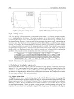
and pattern classification is realized. Figure 2 is a schematic sketch of the architecture of a
fuzzy fusion and classification system for implementing the machine behaviour analysis.
The operational parameters P
1
to P
n
sensed by the multi-sensor arrangement are optionally
preprocessed prior to feeding into the pattern classifier. Such preprocessing may in
particular include a spectral transformation of some of the signals output by the sensors.
Such spectral transformation will in particular be envisaged for processing the signal’s
representative of vibrations or noise produced by the printing press, such as the
characteristic noise or vibration patterns of intaglio printing presses.
Preprocessing
(e.g. spectral transforms)
Sensors
F
u
z
z
y
C
l
a
s
s
i
f
i
e
r
Decision
Unit
1
P
n
P
Fig. 2. Multi-sensor fusion approach based on Fuzzy-Pattern-Classifier modelling
5. Modelling by Fuzzy-Pattern-Classification
Fuzzy set theory, introduced first by Zadeh (Zadeh, 1965), is a framework which adds
uncertainty as an additional feature to aggregation and classification of data. Accepting
vagueness as a key idea in signal measurement and human information processing, fuzzy
membership functions are a suitable basis for modelling information fusion and
classification. An advantage in a fuzzy set approach is that class memberships can be trained
by measured information while simultaneously expert’s know-how can be taken into
account (Bocklisch, 1986).
Fuzzy-Pattern-Classification techniques are used in order to implement the machine
behaviour analysis. In other words, sets of fuzzy-logic rules are applied to characterize the
behaviours of the printing press and model the various classes of printing errors which are
likely to appear on the printing press. Once these fuzzy-logic rules have been defined, they
can be applied to monitor the behaviour of the printing press and identify a possible
correspondence with any machine behaviour which leads or is likely to lead to the
Fuzzy-Pattern-Classier Based Sensor Fusion for Machine Conditioning 327
4.
temperature of a cylinder or roller of the printing press;
5.
pressure between two cylinders or rollers of the printing press;
6.
constraints on bearings of a cylinder or roller of the printing press;
7.
consumption of inks or fluids in the printing press; and/or
8.
position or presence of the processed substrates in the printing press (this latter
information is particularly useful in the context of printing presses comprising of
several printing plates and/or printing blankets as the printing behaviour changes
from one printing plate or blanket to the next).
Depending on the particular configuration of the printing press, it might be useful to
monitor other operational parameters. For example, in the case of an intaglio printing press,
monitoring key components of the so called wiping unit (Lohweg, 2006) has shown to be
particularly useful in order to derive a representative model of the behaviour of the printing
press, as many printing problems in intaglio printing presses are due to a faulty or abnormal
behaviour of the wiping unit.
In general, multiple sensors are combined and mounted on a production machine. One
assumption which is made in such applications is that the sensor signals should be de-
correlated at least in a weak sense. Although this strategy is conclusive, the main drawback
is based on the fact that even experts have only vague information about sensory cross
correlation effects in machines or production systems. Furthermore, many measurements
which are taken traditionally result in ineffective data simply because the measurement
methods are suboptimal.
Therefore, our concept is based on a prefixed data analysis before classifying data. The
classifier’s learning is controlled by the data analysis results. The general concept is based
on the fact that multi-sensory information can be fused with the help of a Fuzzy-Pattern-
Classifier chain, which is described in section 5.
4. Fuzzy Multi-sensor Fusion
It can hardly be said that information fusion is a brand new concept. As a matter of fact, it
has already been used by humans and animals intuitively. Techniques required for
information fusion include various subjects, including artificial intelligence (AI), control
theory, fuzzy logic, and numerical methods and so on. More areas are expected to join in
along with consecutive successful applications invented both in defensive and civilian
fields.
Multi-sensor fusion is the combination of sensory data or data derived from sensory data
and from disparate sources such that the resulting information is in some sense better than
for the case that the sources are used individually, assuming the sensors are combined in a
good way. The term ‘better’ in that case can mean more accurate, more complete, or more
reliable. The fusion procedure can be obtained from direct or indirect fusion.
Direct fusion is
the fusion of sensor data from some homogeneous sensors, such as acoustical sensors;
indirect fusion means the fused knowledge from prior information, which could come from
human inputs. As pointed out above, multi-sensor fusion serves as a very good tool to
obtain better and more reliable outputs, which can facilitate industrial applications and
compensate specialised industrial sub-systems to a large extent.
The primary objective of multivariate data analysis in fusion is to summarise large amounts
of data by means of relatively few parameters. The underlying theme behind many
multivariate techniques is reduction of features. One of these techniques is the Principal
Components Analysis (PCA), which is also known as the Karhunen-Loéve transform (KLT)
(Jolliffe, 2002).
Fuzzy-Pattern-Classification in particular is an effective way to describe and classify the
printing press behaviours into a limited number of classes. It typically partitions the input
space (in the present instance the variables – or operational parameters – sensed by the
multiple sensors provided on functional components of the printing press) into categories or
pattern classes and assigns a given pattern to one of those categories. If a pattern does not fit
directly within a given category, a so-called “goodness of fit” is reported. By employing
fuzzy sets as pattern classes, it is possible to describe the degree to which a pattern belongs
to one class or to another. By viewing each category as a fuzzy set and identifying a set of
fuzzy “if-then” rules as assignment operators, a direct relationship between the fuzzy set
and pattern classification is realized. Figure 2 is a schematic sketch of the architecture of a
fuzzy fusion and classification system for implementing the machine behaviour analysis.
The operational parameters P
1
to P
n
sensed by the multi-sensor arrangement are optionally
preprocessed prior to feeding into the pattern classifier. Such preprocessing may in
particular include a spectral transformation of some of the signals output by the sensors.
Such spectral transformation will in particular be envisaged for processing the signal’s
representative of vibrations or noise produced by the printing press, such as the
characteristic noise or vibration patterns of intaglio printing presses.
Preprocessing
(e.g. spectral transforms)
Sensors
F
u
z
z
y
C
l
a
s
s
i
f
i
e
r
Decision
Unit
1
P
n
P
Fig. 2. Multi-sensor fusion approach based on Fuzzy-Pattern-Classifier modelling
5. Modelling by Fuzzy-Pattern-Classification
Fuzzy set theory, introduced first by Zadeh (Zadeh, 1965), is a framework which adds
uncertainty as an additional feature to aggregation and classification of data. Accepting
vagueness as a key idea in signal measurement and human information processing, fuzzy
membership functions are a suitable basis for modelling information fusion and
classification. An advantage in a fuzzy set approach is that class memberships can be trained
by measured information while simultaneously expert’s know-how can be taken into
account (Bocklisch, 1986).
Fuzzy-Pattern-Classification techniques are used in order to implement the machine
behaviour analysis. In other words, sets of fuzzy-logic rules are applied to characterize the
behaviours of the printing press and model the various classes of printing errors which are
likely to appear on the printing press. Once these fuzzy-logic rules have been defined, they
can be applied to monitor the behaviour of the printing press and identify a possible
correspondence with any machine behaviour which leads or is likely to lead to the
Sensor Fusion and Its Applications328
occurrence of printing errors. Broadly speaking, Fuzzy-Pattern-Classification is a known
technique that concerns the description or classification of measurements. The idea behind
Fuzzy-Pattern-Classification is to define the common features or properties among a set of
patterns (in this case the various behaviours a printing press can exhibit) and classify them
into different predetermined classes according to a determined classification model. Classic
modelling techniques usually try to avoid vague, imprecise or uncertain descriptive rules.
Fuzzy systems deliberately make use of such descriptive rules. Rather than following a
binary approach wherein patterns are defined by “right” or “wrong” rules, fuzzy systems
use relative “if-then” rules of the type “if
parameter alpha is equal to (greater than, …less
than)
value beta, then event A always (often, sometimes, never) happens”. Descriptors
“always”, “often”, “sometimes”, “never” in the above exemplary rule are typically
designated as “linguistic modifiers” and are used to model the desired pattern in a sense of
gradual truth (Zadeh, 1965; Bezdek, 2005). This leads to simpler, more suitable models
which are easier to handle and more familiar to human thinking. In the next sections we will
highlight some Fuzzy-Pattern-Classification approaches which are suitable for sensor fusion
applications.
5.1 Modified-Fuzzy-Pattern-Classification
The Modified-Fuzzy-Pattern-Classifier (MFPC) is a hardware optimized derivate of
Bocklisch’s Fuzzy-Pattern-Classifier (FPC) (Bocklisch, 1986). It should be worth mentioning
here that Hempel and Bocklisch (Hempel, 2010) showed that even non-convex classes can be
modelled within the framework of Fuzzy-Pattern-Classification. The ongoing research on
FPC for non-convex classes make the framework attractive for Support Vector Machine
(SVM) advocates.
Inspired from Eichhorn (Eichhorn, 2000), Lohweg et al. examined both, the FPC and the
MFPC, in detail (Lohweg, 2004). MFPC’s general concept of simultaneously calculating a
number of membership values and aggregating these can be valuably utilised in many
approaches. The author’s intention, which yields to the MFPC in the form of an optimized
structure, was to create a pattern recognition system on a Field Programmable Gate Array
(FPGA) which can be applied in high-speed industrial environments (Lohweg, 2009). As
MFPC is well-suited for industrial implementations, it was already applied in many
applications (Lohweg, 2006; Lohweg, 2006a; Lohweg, 2009; Mönks, 2009; Niederhöfer, 2009).
Based on membership functions
,μ m p , MFPC is employed as a useful approach to
modelling complex systems and classifying noisy data. The originally proposed unimodal
MFPC fuzzy membership function
,μ m p can be described in a graph as:
r
D
)(m
f
B
r
B
r
Cm
0
f
Cm
0
0
m
f
D
m
Fig. 3. Prototype of a unimodal membership function
The prototype of a one-dimensional potential function
,μ m p can be expressed as follows
(Eichhorn, 2000; Lohweg, 2004):
( , )
( , ) 2
d m
m A
p
p ,
(3)
with the difference measure
0
0
0
0
1
1 ,
( , ) .
1
1 ,
r
f
D
r r
D
f f
m m
m m
B C
d m
m m
m m
B C
p
(4)
As for Fig. 3, the potential function
( , )m
p is a function concerning parameters A and the
parameter vector p containing coefficients
0
,m ,
r
B
,
f
B
,
r
C
,
f
C
,
r
D
and .
f
D A is denoted
as the amplitude of this function, and in hardware design usually set 1.A
The coefficient
0
m is featured as center of gravity. The parameters
r
B and
f
B
determine the value of the
membership function on the boundaries
0 r
m C
and
0
f
m C
correspondingly. In addition,
rising and falling edges of this function are described by
0
( , )
r r
m C B
p
and
0
( , ) .
f
f
m C B
p The distance from the center of gravity is interpreted by
r
C and .
f
C The
parameters
r
D and
f
D depict the decrease in membership with the increase of the distance
from the center of gravity
0
.m Suppose there are M features considered, then Eq. 3 can be
reformulated as:
1
0
1
( , )
( , ) 2 .
M
i i i
i
d m
M
p
m p
(5)
With a special definition (
1,A
0.5,
r f
B B
,
r f
C C
r f
D D
) Modified-Fuzzy-Pattern
Classification (Lohweg, 2004; Lohweg 2006; Lohweg 2006a) can be derived as:
Fuzzy-Pattern-Classier Based Sensor Fusion for Machine Conditioning 329
occurrence of printing errors. Broadly speaking, Fuzzy-Pattern-Classification is a known
technique that concerns the description or classification of measurements. The idea behind
Fuzzy-Pattern-Classification is to define the common features or properties among a set of
patterns (in this case the various behaviours a printing press can exhibit) and classify them
into different predetermined classes according to a determined classification model. Classic
modelling techniques usually try to avoid vague, imprecise or uncertain descriptive rules.
Fuzzy systems deliberately make use of such descriptive rules. Rather than following a
binary approach wherein patterns are defined by “right” or “wrong” rules, fuzzy systems
use relative “if-then” rules of the type “if
parameter alpha is equal to (greater than, …less
than)
value beta, then event A always (often, sometimes, never) happens”. Descriptors
“always”, “often”, “sometimes”, “never” in the above exemplary rule are typically
designated as “linguistic modifiers” and are used to model the desired pattern in a sense of
gradual truth (Zadeh, 1965; Bezdek, 2005). This leads to simpler, more suitable models
which are easier to handle and more familiar to human thinking. In the next sections we will
highlight some Fuzzy-Pattern-Classification approaches which are suitable for sensor fusion
applications.
5.1 Modified-Fuzzy-Pattern-Classification
The Modified-Fuzzy-Pattern-Classifier (MFPC) is a hardware optimized derivate of
Bocklisch’s Fuzzy-Pattern-Classifier (FPC) (Bocklisch, 1986). It should be worth mentioning
here that Hempel and Bocklisch (Hempel, 2010) showed that even non-convex classes can be
modelled within the framework of Fuzzy-Pattern-Classification. The ongoing research on
FPC for non-convex classes make the framework attractive for Support Vector Machine
(SVM) advocates.
Inspired from Eichhorn (Eichhorn, 2000), Lohweg et al. examined both, the FPC and the
MFPC, in detail (Lohweg, 2004). MFPC’s general concept of simultaneously calculating a
number of membership values and aggregating these can be valuably utilised in many
approaches. The author’s intention, which yields to the MFPC in the form of an optimized
structure, was to create a pattern recognition system on a Field Programmable Gate Array
(FPGA) which can be applied in high-speed industrial environments (Lohweg, 2009). As
MFPC is well-suited for industrial implementations, it was already applied in many
applications (Lohweg, 2006; Lohweg, 2006a; Lohweg, 2009; Mönks, 2009; Niederhöfer, 2009).
Based on membership functions
,μ m p , MFPC is employed as a useful approach to
modelling complex systems and classifying noisy data. The originally proposed unimodal
MFPC fuzzy membership function
,μ m p can be described in a graph as:
r
D
)(m
f
B
r
B
r
Cm
0
f
Cm
0
0
m
f
D
m
Fig. 3. Prototype of a unimodal membership function
The prototype of a one-dimensional potential function
,μ m p can be expressed as follows
(Eichhorn, 2000; Lohweg, 2004):
( , )
( , ) 2
d m
m A
p
p ,
(3)
with the difference measure
0
0
0
0
1
1 ,
( , ) .
1
1 ,
r
f
D
r r
D
f f
m m
m m
B C
d m
m m
m m
B C
p
(4)
As for Fig. 3, the potential function
( , )m
p is a function concerning parameters A and the
parameter vector p containing coefficients
0
,m ,
r
B
,
f
B
,
r
C
,
f
C
,
r
D
and .
f
D A is denoted
as the amplitude of this function, and in hardware design usually set 1.A
The coefficient
0
m is featured as center of gravity. The parameters
r
B and
f
B
determine the value of the
membership function on the boundaries
0 r
m C and
0
f
m C correspondingly. In addition,
rising and falling edges of this function are described by
0
( , )
r r
m C B
p
and
0
( , ) .
f
f
m C B
p The distance from the center of gravity is interpreted by
r
C and .
f
C The
parameters
r
D and
f
D depict the decrease in membership with the increase of the distance
from the center of gravity
0
.m Suppose there are M features considered, then Eq. 3 can be
reformulated as:
1
0
1
( , )
( , ) 2 .
M
i i i
i
d m
M
p
m p
(5)
With a special definition (
1,A 0.5,
r f
B B ,
r f
C C
r f
D D ) Modified-Fuzzy-Pattern
Classification (Lohweg, 2004; Lohweg 2006; Lohweg 2006a) can be derived as:
Sensor Fusion and Its Applications330
1
0
1
( , )
( , ) 2
M
i i i
i
d m
M
MFPC
p
m p ,
(6)
where
0,
( , ) ,
D
i i
i i i
i
m m
d m
C
p
0, max min
1
( ),
2
i i
i
m m m
max min
(1 2 ) ( ).
2
i i
i CE
m m
C P
(7)
The parameters
max
m and
min
m are the maximum and minimum values of a feature in the
training set. The parameter
i
m is the input feature which is supposed to be classified.
Admittedly, the same objects should have similar feature values that are close to each other.
In such a sense, the resulting value of
0,i i
m m ought to fall into a small interval,
representing their similarity. The value
CE
P is called elementary fuzziness ranging from
zero to one and can be tuned by experts’ know-how. The same implies to D = (2, 4, 8, …).
The aggregation is performed by a fuzzy averaging operation with a subsequent
normalization procedure.
As an instance of FPC, MFPC was addressed and successfully hardware-implemented on
banknote sheet inspection machines. MFPC utilizes the concept of membership functions in
fuzzy set theory and is capable of classifying different objects (data) according to their
features, and the outputs of the membership functions behave as evidence for decision
makers to make judgments. In industrial applications, much attention is paid on the costs
and some other practical issues, thus MFPC is of great importance, particularly because of
its capability to model complex systems and hardware implementability on FPGAs.
5.2 Adaptive Learning Model for Modified-Fuzzy-Pattern-Classification
In this section we present an adaptive learning model for fuzzy classification and sensor
fusion, which on one hand adapts itself to varying data and on the other hand fuses sensory
information to one score value. The approach is based on the following facts:
1.
The sensory data are in general correlated or
2.
Tend to correlate due to material changes in a machine.
3.
The measurement data are time-variant, e.g., in a production process many
parameters are varying imperceptively.
4.
The definition of “good” production is always human-centric. Therefore, a
committed quality standard is defined at the beginning of a production run.
5.
Even if the machine parameters change in a certain range the quality could be in
order.
The underlying scheme is based on membership functions (local classifiers)
( , )
i i i
m
p ,
which are tuned by a learning (training) process. Furthermore, each membership function is
weighted with an attractor value A
i
, which is proportional to the eigenvalue of the
corresponding feature m
i
. This strategy leads to the fact that the local classifiers are trained
based on committed quality and weighted by their attraction specified by a Principal
Component Analysis’ (PCA) (Jolliffe, 2002) eigenvalues. The aggregation is again performed
by a fuzzy averaging operation with a subsequent normalization procedure.
5.2.1 Review on PCA
The Principal Components Analysis (PCA) is effective, if the amount of data is high while
the feature quantity is small (< 30 features). PCA is a way of identifying patterns in data,
and expressing the data in such a way as to highlight their similarities and differences. Since
patterns in data are hard to find in data of high dimensions, where the graphical
representation is not available, PCA is a powerful tool for analysing data. The other main
advantage of PCA is that once patterns in the data are found, it is possible to compress the
data by reducing the number of dimensions without much loss of information. The main
task of the PCA is to project input data into a new (sub-)space, wherein the different input
signals are de-correlated. The PCA is used to find weightings of signal importance in the
measurement’s data set.
PCA involves a mathematical procedure which transforms a set of correlated response
variables into a smaller set of uncorrelated variables called principal components. More
formally it is a linear transformation which chooses a new coordinate system for the data set
such that the greatest variance by any projection of the set is on the first axis, which is also
called the first principal component. The second greatest variance is on the second axis, and
so on. Those created principal component variables are useful for a variety of things
including data screening, assumption checking and cluster verification. There are two
possibilities to perform PCA: first applying PCA to a covariance matrix and second
applying PCA to a correlation matrix. When variables are not normalised, it is necessary to
choose the second approach: Applying PCA to raw data will lead to a false estimation,
because variables with the largest variance will dominate the first principal component.
Therefore in this work the second method in applying PCA to standardized data
(correlation matrix) is presented (Jolliffe, 2002).
In the following the function steps of applying PCA to a correlation matrix is reviewed
concisely. If there are
M
data vectors
1
T T
N MN
x x each of length N , the projection of the
data into a subspace is executed by using the Karhunen-Loéve transform (KLT) and their
inverse, defined as:
T
Y W X and
X W Y , (8)
where
Y is the output matrix, W is the KLT transform matrix followed by the data (input)
matrix:
11 12 1
21 22 2
1 2
N
N
M M MN
x x x
x x x
x x x
X
.
(9)
Furthermore, the expectation value E(•) (average
x ) of the data vectors is necessary:
1
1
2
2
( )
( )
( )
( )
M
M
x
E x
x
E x
E X
x
E x
x , where
1
1
N
i i
i
x x
N
.
(10)
Fuzzy-Pattern-Classier Based Sensor Fusion for Machine Conditioning 331
1
0
1
( , )
( , ) 2
M
i i i
i
d m
M
MFPC
p
m p ,
(6)
where
0,
( , ) ,
D
i i
i i i
i
m m
d m
C
p
0, max min
1
( ),
2
i i
i
m m m
max min
(1 2 ) ( ).
2
i i
i CE
m m
C P
(7)
The parameters
max
m and
min
m are the maximum and minimum values of a feature in the
training set. The parameter
i
m is the input feature which is supposed to be classified.
Admittedly, the same objects should have similar feature values that are close to each other.
In such a sense, the resulting value of
0,i i
m m ought to fall into a small interval,
representing their similarity. The value
CE
P is called elementary fuzziness ranging from
zero to one and can be tuned by experts’ know-how. The same implies to D = (2, 4, 8, …).
The aggregation is performed by a fuzzy averaging operation with a subsequent
normalization procedure.
As an instance of FPC, MFPC was addressed and successfully hardware-implemented on
banknote sheet inspection machines. MFPC utilizes the concept of membership functions in
fuzzy set theory and is capable of classifying different objects (data) according to their
features, and the outputs of the membership functions behave as evidence for decision
makers to make judgments. In industrial applications, much attention is paid on the costs
and some other practical issues, thus MFPC is of great importance, particularly because of
its capability to model complex systems and hardware implementability on FPGAs.
5.2 Adaptive Learning Model for Modified-Fuzzy-Pattern-Classification
In this section we present an adaptive learning model for fuzzy classification and sensor
fusion, which on one hand adapts itself to varying data and on the other hand fuses sensory
information to one score value. The approach is based on the following facts:
1.
The sensory data are in general correlated or
2.
Tend to correlate due to material changes in a machine.
3.
The measurement data are time-variant, e.g., in a production process many
parameters are varying imperceptively.
4.
The definition of “good” production is always human-centric. Therefore, a
committed quality standard is defined at the beginning of a production run.
5.
Even if the machine parameters change in a certain range the quality could be in
order.
The underlying scheme is based on membership functions (local classifiers)
( , )
i i i
m
p ,
which are tuned by a learning (training) process. Furthermore, each membership function is
weighted with an attractor value A
i
, which is proportional to the eigenvalue of the
corresponding feature m
i
. This strategy leads to the fact that the local classifiers are trained
based on committed quality and weighted by their attraction specified by a Principal
Component Analysis’ (PCA) (Jolliffe, 2002) eigenvalues. The aggregation is again performed
by a fuzzy averaging operation with a subsequent normalization procedure.
5.2.1 Review on PCA
The Principal Components Analysis (PCA) is effective, if the amount of data is high while
the feature quantity is small (< 30 features). PCA is a way of identifying patterns in data,
and expressing the data in such a way as to highlight their similarities and differences. Since
patterns in data are hard to find in data of high dimensions, where the graphical
representation is not available, PCA is a powerful tool for analysing data. The other main
advantage of PCA is that once patterns in the data are found, it is possible to compress the
data by reducing the number of dimensions without much loss of information. The main
task of the PCA is to project input data into a new (sub-)space, wherein the different input
signals are de-correlated. The PCA is used to find weightings of signal importance in the
measurement’s data set.
PCA involves a mathematical procedure which transforms a set of correlated response
variables into a smaller set of uncorrelated variables called principal components. More
formally it is a linear transformation which chooses a new coordinate system for the data set
such that the greatest variance by any projection of the set is on the first axis, which is also
called the first principal component. The second greatest variance is on the second axis, and
so on. Those created principal component variables are useful for a variety of things
including data screening, assumption checking and cluster verification. There are two
possibilities to perform PCA: first applying PCA to a covariance matrix and second
applying PCA to a correlation matrix. When variables are not normalised, it is necessary to
choose the second approach: Applying PCA to raw data will lead to a false estimation,
because variables with the largest variance will dominate the first principal component.
Therefore in this work the second method in applying PCA to standardized data
(correlation matrix) is presented (Jolliffe, 2002).
In the following the function steps of applying PCA to a correlation matrix is reviewed
concisely. If there are
M
data vectors
1
T T
N MN
x x each of length N , the projection of the
data into a subspace is executed by using the Karhunen-Loéve transform (KLT) and their
inverse, defined as:
T
Y W X and X W Y , (8)
where
Y is the output matrix, W is the KLT transform matrix followed by the data (input)
matrix:
11 12 1
21 22 2
1 2
N
N
M M MN
x x x
x x x
x x x
X
.
(9)
Furthermore, the expectation value E(•) (average
x ) of the data vectors is necessary:
1
1
2
2
( )
( )
( )
( )
M
M
x
E x
x
E x
E X
x
E x
x , where
1
1
N
i i
i
x x
N
.
(10)
Sensor Fusion and Its Applications332
With the help of the data covariance matrix
11 12 1
21 22 2
1 2
( )( )
M
M
T
M M MM
c c c
c c c
E
c c
C x x x x
,
(11)
the correlation matrix
R is calculated by:
12 1
21 2
1 2
1
1
1
N
N
N N
R , where
ij
ij
ii
jj
c
c c
.
(12)
The variables
ii
c are called variances; the variables
i
j
c are called covariances of a data set.
The correlation coefficients are described as
i
j
. Correlation is a measure of the relation
between two or more variables. Correlation coefficients can range from -1 to +1. The value
of -1 represents a perfect negative correlation while a value of +1 represents a perfect
positive correlation. A value of 0 represents no correlation. In the next step the eigenvalues
i
and the eigenvectors V of the correlation matrix are computed by Eq. 13, where
dia
g
( )
is the diagonal matrix of eigenvalues of C:
1
diag( )
V R V .
(13)
The eigenvectors generate the KLT matrix and the eigenvalues represent the distribution of
the source data's energy among each of the eigenvectors. The cumulative energy content for
the pth eigenvector is the sum of the energy content across all of the eigenvectors from 1
through p. The eigenvalues have to be sorted in decreasing order:
1
0
0
M
, where
1 2
M
.
(14)
The corresponding vectors
i
v of the matrix V have also to be sorted in decreasing order
like the eigenvalues, where
1
v is the first column of matrix V ,
2
v the second and
M
v is the
last column of matrix
V . The eigenvector
1
v corresponds to eigenvalue
1
, eigenvector
2
v
to eigenvalue
2
and so forth. The matrix W represents a subset of the column eigenvectors
as basis vectors. The subset is preferably as small as possible (two eigenvectors). The energy
distribution is a good indicator for choosing the number of eigenvectors. The cumulated
energy should map approx. 90
% on a low number of eigenvectors. The matrix
Y
(cf. Eq. 8)
then represents the Karhunen-Loéve transformed data (KLT) of matrix
X (Lohweg, 2006a).
5.2.2 Modified Adaptive-Fuzzy-Pattern-Classifier
The adaptive Fuzzy-Pattern-Classifier core based on the world model (Luo, 1989) consists of
M local classifiers (MFPC), one for each feature. It can be defined as
1 1 1
2 2 2
, 0 0 0
0 , 0 0
0 0 0
0 0 0 ,
i
M M M
m
m
AFPC diag
m
p
p
p
.
(15)
The adaptive fuzzy inference system (AFIS), is then described with a length M unit vector
1, , 1
T
u and the attractor vector
1 2
, , ,
T
M
A A AA as
1
T
AFIS i
T
diagA u
A u
,
(16)
which can be written as
1
1
1
2
i
M
d
AFIS i
M
i
i
i
A
A
.
(17)
The adaptive Fuzzy-Pattern-Classifier model output
A
FIS
can be interpreted as a score value
in the range of
0 1 . If 1
AFIS
, a perfect match is reached, which can be assumed as a
measure for a “good” system state, based on an amount of sensor signals. The score value
0
AFIS
represents the overall “bad” measure decision for a certain trained model. As it
will be explained in section 6 the weight values of each parameter are taken as the weighted
components of eigenvector one (PC1) times the square roots of the corresponding
eigenvalues:
1 1
i i
A v .
(18)
With Eq. 17 the Modified-Adaptive-Fuzzy-Pattern-Classifier (MAFPC) results then in
1 1
1
1 1
1
1
2
i
M
d
MAFPC i
M
i
i
i
v
v
.
(19)
In section 6.1 an application with MAFPC will be highlighted.
5.3 Probabilistic Modified-Fuzzy-Pattern-Classifier
In many knowledge-based industrial applications there is a necessity to train using a small
data set. It is typical that there are less than ten up to some tens of training examples.
Having only such a small data set, the description of the underlying universal set, from
which these examples are taken, is very vague and connected to a high degree of
uncertainty. The heuristic parameterisation methods for the MFPC presented in section 5.1
leave a high degree of freedom to the user which makes it hard to find optimal parameter
values. In this section we suggest an automatic method of learning the fuzzy membership
Fuzzy-Pattern-Classier Based Sensor Fusion for Machine Conditioning 333
With the help of the data covariance matrix
11 12 1
21 22 2
1 2
( )( )
M
M
T
M M MM
c c c
c c c
E
c c
C x x x x
,
(11)
the correlation matrix
R is calculated by:
12 1
21 2
1 2
1
1
1
N
N
N N
R , where
ij
ij
ii
jj
c
c c
.
(12)
The variables
ii
c are called variances; the variables
i
j
c are called covariances of a data set.
The correlation coefficients are described as
i
j
. Correlation is a measure of the relation
between two or more variables. Correlation coefficients can range from -1 to +1. The value
of -1 represents a perfect negative correlation while a value of +1 represents a perfect
positive correlation. A value of 0 represents no correlation. In the next step the eigenvalues
i
and the eigenvectors V of the correlation matrix are computed by Eq. 13, where
dia
g
( )
is the diagonal matrix of eigenvalues of C:
1
diag( )
V R V .
(13)
The eigenvectors generate the KLT matrix and the eigenvalues represent the distribution of
the source data's energy among each of the eigenvectors. The cumulative energy content for
the pth eigenvector is the sum of the energy content across all of the eigenvectors from 1
through p. The eigenvalues have to be sorted in decreasing order:
1
0
0
M
, where
1 2
M
.
(14)
The corresponding vectors
i
v of the matrix V have also to be sorted in decreasing order
like the eigenvalues, where
1
v is the first column of matrix V ,
2
v the second and
M
v is the
last column of matrix
V . The eigenvector
1
v corresponds to eigenvalue
1
, eigenvector
2
v
to eigenvalue
2
and so forth. The matrix W represents a subset of the column eigenvectors
as basis vectors. The subset is preferably as small as possible (two eigenvectors). The energy
distribution is a good indicator for choosing the number of eigenvectors. The cumulated
energy should map approx. 90
% on a low number of eigenvectors. The matrix
Y
(cf. Eq. 8)
then represents the Karhunen-Loéve transformed data (KLT) of matrix
X (Lohweg, 2006a).
5.2.2 Modified Adaptive-Fuzzy-Pattern-Classifier
The adaptive Fuzzy-Pattern-Classifier core based on the world model (Luo, 1989) consists of
M local classifiers (MFPC), one for each feature. It can be defined as
1 1 1
2 2 2
, 0 0 0
0 , 0 0
0 0 0
0 0 0 ,
i
M M M
m
m
AFPC diag
m
p
p
p
.
(15)
The adaptive fuzzy inference system (AFIS), is then described with a length M unit vector
1, , 1
T
u and the attractor vector
1 2
, , ,
T
M
A A AA as
1
T
AFIS i
T
diagA u
A u
,
(16)
which can be written as
1
1
1
2
i
M
d
AFIS i
M
i
i
i
A
A
.
(17)
The adaptive Fuzzy-Pattern-Classifier model output
A
FIS
can be interpreted as a score value
in the range of
0 1 . If 1
AFIS
, a perfect match is reached, which can be assumed as a
measure for a “good” system state, based on an amount of sensor signals. The score value
0
AFIS
represents the overall “bad” measure decision for a certain trained model. As it
will be explained in section 6 the weight values of each parameter are taken as the weighted
components of eigenvector one (PC1) times the square roots of the corresponding
eigenvalues:
1 1
i i
A v .
(18)
With Eq. 17 the Modified-Adaptive-Fuzzy-Pattern-Classifier (MAFPC) results then in
1 1
1
1 1
1
1
2
i
M
d
MAFPC i
M
i
i
i
v
v
.
(19)
In section 6.1 an application with MAFPC will be highlighted.
5.3 Probabilistic Modified-Fuzzy-Pattern-Classifier
In many knowledge-based industrial applications there is a necessity to train using a small
data set. It is typical that there are less than ten up to some tens of training examples.
Having only such a small data set, the description of the underlying universal set, from
which these examples are taken, is very vague and connected to a high degree of
uncertainty. The heuristic parameterisation methods for the MFPC presented in section 5.1
leave a high degree of freedom to the user which makes it hard to find optimal parameter
values. In this section we suggest an automatic method of learning the fuzzy membership
Sensor Fusion and Its Applications334
functions by estimating the data set's probability distribution and deriving the function's
parameters automatically from it. The resulting Probabilistic MFPC (PMFPC) membership
function is based on the MFPC approach, but leaves only one degree of freedom leading to a
shorter learning time for obtaining stable and robust classification results (Mönks, 2010).
Before obtaining the different PMFPC formulation, it is reminded that the membership
functions are aggregated using a fuzzy averaging operator in the MFPC approach.
Consequently, on the one hand the PMFPC membership functions can substitute the MFPC
membership function. On the other hand the fuzzy averaging operator used in the MFPC
can be substituted by any other operator. Actually, it is also possible to substitute both parts
of the MFPC at the same time (Mönks, 2010), and in all cases the application around the
classifier remains unchanged. To achieve the possibility of exchanging the MFPC’s core
parts, its formulation of Eq. 6 is rewritten to
1
0
1
1
( , )
( , )
1
( , ) 2 2
M
i i i
i i i
i
M
d m
M
M
d m
MFPC
i
p
p
m p ,
(20)
revealing that the MFPC incorporates the geometric mean as its fuzzy averaging operator.
Also, the unimodal membership function, as introduced in Eq. 3 with
1A , is isolated
clearly, which shall be replaced by the PMFPC membership function described in the
following section.
5.3.1 Probabilistic MFPC Membership Function
The PMFPC approach is based on a slightly modified MFPC membership function
1
,
( , ) 2 0,1
ld d m
B
m
p
p .
(21)
D and B are automatically parameterised in the PMFPC approach.
CE
P
is yet not automated
to preserve the possibility of adjusting the membership function slightly without needing to
learn the membership functions from scratch. The algorithms presented here for
automatically parameterising parameters
D and B are inspired by former approaches:
Bocklisch as well as Eichhorn developed algorithms which allow obtaining a value for the
(MFPC) potential function's parameter
D automatically, based on the used training data set.
Bocklisch also proposed an algorithm for the determination of
B. For details we refer to
(Bocklisch, 1987) and (Eichhorn, 2000). However, these algorithms yield parameters that do
not fulfil the constraints connected with them in all practical cases (cf. (Mönks, 2010)).
Hence, we propose a probability theory-based alternative described in the following.
Bocklisch's and Eichhorn's algorithms adjust
D after comparing the actual distribution of
objects to a perfect uniform distribution. However, the algorithms tend to change
D for
every (small) difference between the actual distribution and a perfect uniform distribution.
This explains why both algorithms do not fulfil the constraints when applied to random
uniform distributions.
We actually stick to the idea of adjusting
D with respect to the similarity of the actual
distribution compared to an artificial, ideal uniform distribution, but we use probability
theoretical concepts. Our algorithm basically works as follows: At first, the empirical
cumulative distribution function (ECDF) of the data set under investigation is determined.
Then, the ECDF of an artificial perfect uniform distribution in the range of the actual
distribution is determined, too. The similarity between both ECDFs is expressed by its
correlation factor which is subsequently mapped to
D by a parameterisable function.
5.3.1.1 Determining the Distributions’ Similarity
Consider a sorted vector of n feature values
1 2
, , ,
n
m m mm with
1 2 n
m m m , thus
min 1
m m and
max n
m m . The corresponding empirical cumulative distribution function
( )
m
P x
is determined by ( )
m
n
P x
m
with
i i n
m m x i m
, where x denotes the
number of elements in vector x and
1,2, ,
n
n . The artificial uniform distribution is
created by equidistantly distributing
n values
i
u , hence
1 2
, , ,
n
u u uu , with
1
1
1
1
m m
n
i
n
u m i
. Its ECDF
( )
u
P x
is determined analogously by substituting m with u.
In the next step, the similarity between both distribution functions is computed by
calculating the
correlation factor (Polyanin, 2007)
1
2 2
1 1
k
m i m u i u
i
k k
m i m u i u
i i
P x P P x P
c
P x P P x P
,
(22)
where
a
P
is the mean value of
a
P x , computed as
1
1
k
a a i
k
i
P P x
. The correlation factor
must now be mapped to
D while fulfilling Bocklisch’s constraints on D (Bocklisch, 1987).
Therefore, the average influence
D
of the parameter D on the MFPC membership
function, which is the base for PMFPC membership function, is investigated to derive a
mapping based on it. First
D
x
is determined by taking ( , )
D
x D
with
0
,
m m
C
x
0x :
( , ) 2 ln(2) 2 ln( )
D D
x x D
D
D D
x x D x x
.
(23)
The locations
x represent the distance to the membership function’s mean value
0
m , hence
0
x is the mean value itself, 1x
is the class boundary
0
m C
, 2x
twice the class
boundary and so on. The average influence of
D on the membership function
1
( ) ( )
r
r l
l
x
D
x x
x
D x dx
is evaluated for 1 1x
: This interval bears the most valuable
information since all feature values of the objects in the training data set are included in this
interval, and additionally those of the class members are expected here during the
classification process, except from only a typically neglectable number of outliers. The
mapping of
: 2,20D c , which is derived in the following, must take D’s average
influence into consideration, which turns out to be exponentially decreasing (Mönks, 2010).
Fuzzy-Pattern-Classier Based Sensor Fusion for Machine Conditioning 335
functions by estimating the data set's probability distribution and deriving the function's
parameters automatically from it. The resulting Probabilistic MFPC (PMFPC) membership
function is based on the MFPC approach, but leaves only one degree of freedom leading to a
shorter learning time for obtaining stable and robust classification results (Mönks, 2010).
Before obtaining the different PMFPC formulation, it is reminded that the membership
functions are aggregated using a fuzzy averaging operator in the MFPC approach.
Consequently, on the one hand the PMFPC membership functions can substitute the MFPC
membership function. On the other hand the fuzzy averaging operator used in the MFPC
can be substituted by any other operator. Actually, it is also possible to substitute both parts
of the MFPC at the same time (Mönks, 2010), and in all cases the application around the
classifier remains unchanged. To achieve the possibility of exchanging the MFPC’s core
parts, its formulation of Eq. 6 is rewritten to
1
0
1
1
( , )
( , )
1
( , ) 2 2
M
i i i
i i i
i
M
d m
M
M
d m
MFPC
i
p
p
m p ,
(20)
revealing that the MFPC incorporates the geometric mean as its fuzzy averaging operator.
Also, the unimodal membership function, as introduced in Eq. 3 with
1A , is isolated
clearly, which shall be replaced by the PMFPC membership function described in the
following section.
5.3.1 Probabilistic MFPC Membership Function
The PMFPC approach is based on a slightly modified MFPC membership function
1
,
( , ) 2 0,1
ld d m
B
m
p
p .
(21)
D and B are automatically parameterised in the PMFPC approach.
CE
P
is yet not automated
to preserve the possibility of adjusting the membership function slightly without needing to
learn the membership functions from scratch. The algorithms presented here for
automatically parameterising parameters
D and B are inspired by former approaches:
Bocklisch as well as Eichhorn developed algorithms which allow obtaining a value for the
(MFPC) potential function's parameter
D automatically, based on the used training data set.
Bocklisch also proposed an algorithm for the determination of
B. For details we refer to
(Bocklisch, 1987) and (Eichhorn, 2000). However, these algorithms yield parameters that do
not fulfil the constraints connected with them in all practical cases (cf. (Mönks, 2010)).
Hence, we propose a probability theory-based alternative described in the following.
Bocklisch's and Eichhorn's algorithms adjust
D after comparing the actual distribution of
objects to a perfect uniform distribution. However, the algorithms tend to change
D for
every (small) difference between the actual distribution and a perfect uniform distribution.
This explains why both algorithms do not fulfil the constraints when applied to random
uniform distributions.
We actually stick to the idea of adjusting
D with respect to the similarity of the actual
distribution compared to an artificial, ideal uniform distribution, but we use probability
theoretical concepts. Our algorithm basically works as follows: At first, the empirical
cumulative distribution function (ECDF) of the data set under investigation is determined.
Then, the ECDF of an artificial perfect uniform distribution in the range of the actual
distribution is determined, too. The similarity between both ECDFs is expressed by its
correlation factor which is subsequently mapped to
D by a parameterisable function.
5.3.1.1 Determining the Distributions’ Similarity
Consider a sorted vector of n feature values
1 2
, , ,
n
m m mm with
1 2 n
m m m , thus
min 1
m m and
max n
m m . The corresponding empirical cumulative distribution function
( )
m
P x
is determined by ( )
m
n
P x
m
with
i i n
m m x i m
, where x denotes the
number of elements in vector x and
1,2, ,
n
n . The artificial uniform distribution is
created by equidistantly distributing
n values
i
u , hence
1 2
, , ,
n
u u uu , with
1
1
1
1
m m
n
i
n
u m i
. Its ECDF
( )
u
P x
is determined analogously by substituting m with u.
In the next step, the similarity between both distribution functions is computed by
calculating the
correlation factor (Polyanin, 2007)
1
2 2
1 1
k
m i m u i u
i
k k
m i m u i u
i i
P x P P x P
c
P x P P x P
,
(22)
where
a
P
is the mean value of
a
P x , computed as
1
1
k
a a i
k
i
P P x
. The correlation factor
must now be mapped to
D while fulfilling Bocklisch’s constraints on D (Bocklisch, 1987).
Therefore, the average influence
D
of the parameter D on the MFPC membership
function, which is the base for PMFPC membership function, is investigated to derive a
mapping based on it. First
D
x
is determined by taking ( , )
D
x D
with
0
,
m m
C
x
0x :
( , ) 2 ln(2) 2 ln( )
D D
x x D
D
D D
x x D x x
.
(23)
The locations
x represent the distance to the membership function’s mean value
0
m , hence
0
x is the mean value itself, 1x is the class boundary
0
m C
, 2x twice the class
boundary and so on. The average influence of
D on the membership function
1
( ) ( )
r
r l
l
x
D
x x
x
D x dx
is evaluated for 1 1x : This interval bears the most valuable
information since all feature values of the objects in the training data set are included in this
interval, and additionally those of the class members are expected here during the
classification process, except from only a typically neglectable number of outliers. The
mapping of
: 2,20D c , which is derived in the following, must take D’s average
influence into consideration, which turns out to be exponentially decreasing (Mönks, 2010).
Sensor Fusion and Its Applications336
5.3.1.2 Mapping the Distributions’ Similarity to the Edge’s Steepness
In the general case, the correlation factor c can take values from the interval
1,1 , but
when evaluating distribution functions, the range of values is restricted to
0,1c , which is
because probability distribution functions are monotonically increasing. This holds for both
distributions,
( )
m
P x as well as ( )
u
P x . It follows 0c . The interpretation of the correlation
factor is straight forward. A high value of c means that the distribution
( )
m
P x
is close to a
uniform distribution. If
( )
m
P x actually was a uniform distribution, 1c since ( ) ( )
m u
P x P x .
According to Bocklisch, D should take a high value here. The more
( )
m
P x differs from a
uniform distribution, the more 0c , the more 2D . Hence, the mapping function
( )D c
must necessarily be an increasing function with taking the exponentially decreasing average
influence of D on the membership function
D
into consideration (cf. (Mönks, 2010)). An
appropriate mapping
: 2,20D c is an exponentially increasing function which
compensates the changes of the MFPC membership function with respect to changes of c.
We suggest the following heuristically determined exponential function, which achieved
promising results during experiments:
2
( ) 19 1 ( ) 2,20
q
c
D c D c ,
(24)
where q is an adjustment parameter. This formulation guarantees that
2,20D c since
0,1c . Using the adjustment parameter q, D is adjusted with respect to the aggregation
operator used to fuse all n membership functions representing each of the n features. Each
fuzzy aggregation operator behaves differently. For a fuzzy averaging operator
( )h a ,
Dujmović introduced the objective measure of global andness
g
(for details cf. (Dujmović,
2007), (Mönks, 2009)). Assuming
1q
in the following cases, it can be observed that, when
using aggregation operators with a global andness
( )
0
h
g
a
, the aggregated single, n-
dimensional membership function is more fuzzy than that one obtained when using an
aggregation operator with
( )
1
h
g
a
, where the resulting function is sharp. This behaviour
should be compensated by adjusting D in such a way, that the aggregated membership
functions have comparable shapes: at some given correlation factor c, D must be increased if
g
is high and vice versa. This is achieved by mapping the aggregation operator’s global
andness to q, hence :
g
q
. Our suggested solution is a direct mapping of the global
andness to the adjustment parameter q, hence
( ) 0,1
g g
q q
. The mapping in Eq. 24
is now completely defined and consistent with Bocklisch’s constraints and the observations
regarding the aggregation operator’s andness.
5.3.1.3 Determining the Class Boundary Membership Parameter
In addition to the determination of D, we present an algorithm to automatically
parameterise the class boundary membership B. This parameter is a measure for the
membership
( , )m
p at the locations
0 0
,m m C m C . The algorithm for determining B
is based on the algorithm Bocklisch developed, but was not adopted as it stands since it has
some disadvantages if this algorithm is applied to distributions with a high density
especially on the class boundaries. For details cf. (Bocklisch, 1987).
When looking at the MFPC membership functions, the following two constraints on B can
be derived: (i) The probability of occurrence is the same for every object in uniform
distributions, also on the class boundary. Here, B should have a high value. (ii) For
distributions where the density of objects decreases when going towards the class
boundaries B should be assigned a small value, since the probability that an object occurs at
the boundary is smaller than in the centre.
Hence, for sharp membership functions ( 20D ) a high value for B should be assigned,
while for fuzzy membership functions ( 2D ) the value of B should be low.
( )B f D must
have similar properties like
D
, meaning B changes quickly where
D
changes
quickly and vice versa. We adopted Bocklisch’s suitable equation for computing the class
boundary membership (Bocklisch, 1987):
1
1
max
max
1
1
1 1
q
B
D
B D
,
(25)
where
max
(0,1)B stands for the maximum possible value of B with a proposed value of 0.9,
max
20D
is the maximum possible value of D and q is identical in its meaning and value to
q as used in Eq. 24.
5.3.1.4 An Asymmetric PMFPC Membership Function Formulation
A data set may be represented better if the membership function was formulated
asymmetrically instead of symmetrically as is the case with Eq. 21. This means
0
0
1
0
1
0
2 ,
( , )
2 ,
D
r
r r
D
f
f f
m m
ld
B C
m m
ld
B C
m m
m
m m
p ,
(26)
where
1
0
1
M
i
M
i
m m
,
i
m
m is the arithmetic mean of all feature values. If
0
m was
computed as introduced in Eq. 7, the resulting membership function would not describe the
underlying feature vector
m appropriately for asymmetrical feature distributions. A new
computation method must therefore also be applied to
0 min max min
( )
r CE
C m m P m m
and
max 0 max min
( )
f CE
C m m P m m due to the change to the asymmetrical formulation.
To compute the remaining parameters, the feature vector must be split into the left side
feature vector
0
( )
r i i
m m m m and the one for the right side
0
( )
f i i
m m m m for all
i
m m
. They are determined following the algorithms presented in the preceding sections
5.3.1.2 and 5.3.1.3, but using only the feature vector for one side to compute this side’s
respective parameter.
Using Eq. 26 as membership function, the Probabilistic Modified-Fuzzy-Pattern-Classifier is
defined as
Fuzzy-Pattern-Classier Based Sensor Fusion for Machine Conditioning 337
5.3.1.2 Mapping the Distributions’ Similarity to the Edge’s Steepness
In the general case, the correlation factor c can take values from the interval
1,1 , but
when evaluating distribution functions, the range of values is restricted to
0,1c , which is
because probability distribution functions are monotonically increasing. This holds for both
distributions,
( )
m
P x as well as ( )
u
P x . It follows 0c . The interpretation of the correlation
factor is straight forward. A high value of c means that the distribution
( )
m
P x
is close to a
uniform distribution. If
( )
m
P x actually was a uniform distribution, 1c
since ( ) ( )
m u
P x P x .
According to Bocklisch, D should take a high value here. The more
( )
m
P x differs from a
uniform distribution, the more 0c , the more 2D . Hence, the mapping function
( )D c
must necessarily be an increasing function with taking the exponentially decreasing average
influence of D on the membership function
D
into consideration (cf. (Mönks, 2010)). An
appropriate mapping
: 2,20D c is an exponentially increasing function which
compensates the changes of the MFPC membership function with respect to changes of c.
We suggest the following heuristically determined exponential function, which achieved
promising results during experiments:
2
( ) 19 1 ( ) 2,20
q
c
D c D c ,
(24)
where q is an adjustment parameter. This formulation guarantees that
2,20D c since
0,1c . Using the adjustment parameter q, D is adjusted with respect to the aggregation
operator used to fuse all n membership functions representing each of the n features. Each
fuzzy aggregation operator behaves differently. For a fuzzy averaging operator
( )h a ,
Dujmović introduced the objective measure of global andness
g
(for details cf. (Dujmović,
2007), (Mönks, 2009)). Assuming
1q
in the following cases, it can be observed that, when
using aggregation operators with a global andness
( )
0
h
g
a
, the aggregated single, n-
dimensional membership function is more fuzzy than that one obtained when using an
aggregation operator with
( )
1
h
g
a
, where the resulting function is sharp. This behaviour
should be compensated by adjusting D in such a way, that the aggregated membership
functions have comparable shapes: at some given correlation factor c, D must be increased if
g
is high and vice versa. This is achieved by mapping the aggregation operator’s global
andness to q, hence :
g
q
. Our suggested solution is a direct mapping of the global
andness to the adjustment parameter q, hence
( ) 0,1
g g
q q
. The mapping in Eq. 24
is now completely defined and consistent with Bocklisch’s constraints and the observations
regarding the aggregation operator’s andness.
5.3.1.3 Determining the Class Boundary Membership Parameter
In addition to the determination of D, we present an algorithm to automatically
parameterise the class boundary membership B. This parameter is a measure for the
membership
( , )m
p at the locations
0 0
,m m C m C . The algorithm for determining B
is based on the algorithm Bocklisch developed, but was not adopted as it stands since it has
some disadvantages if this algorithm is applied to distributions with a high density
especially on the class boundaries. For details cf. (Bocklisch, 1987).
When looking at the MFPC membership functions, the following two constraints on B can
be derived: (i) The probability of occurrence is the same for every object in uniform
distributions, also on the class boundary. Here, B should have a high value. (ii) For
distributions where the density of objects decreases when going towards the class
boundaries B should be assigned a small value, since the probability that an object occurs at
the boundary is smaller than in the centre.
Hence, for sharp membership functions ( 20D ) a high value for B should be assigned,
while for fuzzy membership functions ( 2D ) the value of B should be low.
( )B f D must
have similar properties like
D
, meaning B changes quickly where
D
changes
quickly and vice versa. We adopted Bocklisch’s suitable equation for computing the class
boundary membership (Bocklisch, 1987):
1
1
max
max
1
1
1 1
q
B
D
B D
,
(25)
where
max
(0,1)B stands for the maximum possible value of B with a proposed value of 0.9,
max
20D
is the maximum possible value of D and q is identical in its meaning and value to
q as used in Eq. 24.
5.3.1.4 An Asymmetric PMFPC Membership Function Formulation
A data set may be represented better if the membership function was formulated
asymmetrically instead of symmetrically as is the case with Eq. 21. This means
0
0
1
0
1
0
2 ,
( , )
2 ,
D
r
r r
D
f
f f
m m
ld
B C
m m
ld
B C
m m
m
m m
p ,
(26)
where
1
0
1
M
i
M
i
m m
,
i
m m is the arithmetic mean of all feature values. If
0
m was
computed as introduced in Eq. 7, the resulting membership function would not describe the
underlying feature vector
m appropriately for asymmetrical feature distributions. A new
computation method must therefore also be applied to
0 min max min
( )
r CE
C m m P m m
and
max 0 max min
( )
f CE
C m m P m m due to the change to the asymmetrical formulation.
To compute the remaining parameters, the feature vector must be split into the left side
feature vector
0
( )
r i i
m m m m and the one for the right side
0
( )
f i i
m m m m for all
i
m m
. They are determined following the algorithms presented in the preceding sections
5.3.1.2 and 5.3.1.3, but using only the feature vector for one side to compute this side’s
respective parameter.
Using Eq. 26 as membership function, the Probabilistic Modified-Fuzzy-Pattern-Classifier is
defined as
Sensor Fusion and Its Applications338
0
0
1
1
0
1
1
1
0
1
2 ,
( , )
2 ,
D
r
r r
D
f
f
M
m m
ld
M
B C
i
PMFPC
M
m m
ld
M
B C
f
i
m m
m m
m p ,
(27)
having in mind, that the geometric mean operator can be substituted by any other fuzzy
averaging operator. An application is presented in section 6.2.
6. Applications
6.1 Machine Condition Monitoring
The approach presented in section 4 and 5.1 was tested in particular with an intaglio
printing machine in a production process. As an interesting fact print flaws were detected at
an early stage by using multi-sensory measurements. It has to be noted that one of the most
common type of print flaws (Lohweg, 2006) caused by the wiping unit was detected at a
very early stage.
The following data are used for the model: machine speed - motor current - printing
pressure side 1 (PPS1) - printing pressure side 2 (PPS2) - hydraulic pressure (drying blade) -
wiping solution flow - drying blade side 1 (DBS1) - drying blade side 2 (DBS2) - acoustic
signal (vertical side 1) - acoustic signal (horizontal side 1) - acoustic signal (vertical side 2) -
acoustic signal (horizontal side 1).
It has been mentioned that it might be desirable to preprocess some of the signals output by
the sensors which are used to monitor the behaviour of the machine. This is particularly true
in connection with the sensing of noises and/or vibrations produced by the printing press,
which signals a great number of frequency components. The classical approach to
processing such signals is to perform a spectral transformation of the signals. The usual
spectral transformation is the well-known Fourier transform (and derivatives thereof) which
converts the signals from the time-domain into the frequency-domain. The processing of the
signals is made simpler by working in the thus obtained spectrum as periodic signal
components are readily identifiable in the frequency-domain as peaks in the spectrum. The
drawbacks of the Fourier transform, however, reside in its inability to efficiently identify
and isolate phase movements, shifts, drifts, echoes, noise, etc., in the signals. A more
adequate “spectral” analysis is the so-called “cepstrum” analysis. “Cepstrum” is an
anagram of “spectrum” and is the accepted terminology for the inverse Fourier transform of
the logarithm of the spectrum of a signal. Cepstrum analysis is in particular used for
analysing “sounds” instead of analysing frequencies (Bogert, 1963).
A test was performed by measuring twelve different parameters of the printing machine’s
condition while the machine was running (data collection) (Dyck, 2006). During this test the
wiping pressure was decreased little by little, as long as the machine was printing only error
sheets. The test was performed at a speed of 6500 sheets per hour and a sample frequency of
7 kHz. During this test 797 sheets were printed, that means, the set of data contained more
than three million values per signal. In the first step before calculating the KLT of the raw
data, the mean value per sheet was calculated to reduce the amount of data to 797 values
per signal. As already mentioned, 12 signals were measured; therefore the four acoustical
signals were divided by cepstrum analysis in six new parameters, so that all in all 14
parameters built up the new input vectors of matrix
X . As described above, at first the
correlation matrix of the input data was calculated. Some parameters are highly correlated,
e.g. PPS1 and PPS2 with a correlation factor 0.9183, DBS1 and DBS2 with a correlation factor
0.9421, and so forth. This fact already leads to the assumption that implementing the KLT
seems to be effective in reducing the dimensions of the input data. The classifier model is
shown in Fig. 4.
The KLT matrix is given by calculating the eigenvectors and eigenvalues of the correlation
matrix, because the eigenvectors build up the transformation matrix. In Fig. 5 the calculated
eigenvalues are presented. On the ordinate the variance contribution of several eigenvalues
in percentage are plotted versus the number of eigenvalues on the abscissa axis. The first
principal component has already a contribution of almost 60
% of the total variance. Looking
at the first seven principal components, which cover nearly 95
% of the total variance, shows
that this transformation allows a reduction of important parameters for further use in
classification without relevant loss of information. The following implementations focussed
only on the first principal component, which represents the machine condition state best.
Fig. 4. The adaptive Fuzzy-Pattern-Classifier Model. The FPC is trained with 14 features,
while the fuzzy inference system is adapted by the PCA output. Mainly the first principal
component is applied.
PCA is not only a dimension-reducing technique, but also a technique for graphical
representations of high-dimension data. Graphical representation of variables in a two-
dimensional way shows which parameters are correlated. The coordinates of the parameter
are calculated by weighting the components of the eigenvectors with the square root of the
eigenvalues: the ith parameter is represented as the point (
1 1 2 2
,
i i
v v ). This weighting
is executed for normalisation.
Fuzzy-Pattern-Classier Based Sensor Fusion for Machine Conditioning 339
0
0
1
1
0
1
1
1
0
1
2 ,
( , )
2 ,
D
r
r r
D
f
f
M
m m
ld
M
B C
i
PMFPC
M
m m
ld
M
B C
f
i
m m
m m
m p ,
(27)
having in mind, that the geometric mean operator can be substituted by any other fuzzy
averaging operator. An application is presented in section 6.2.
6. Applications
6.1 Machine Condition Monitoring
The approach presented in section 4 and 5.1 was tested in particular with an intaglio
printing machine in a production process. As an interesting fact print flaws were detected at
an early stage by using multi-sensory measurements. It has to be noted that one of the most
common type of print flaws (Lohweg, 2006) caused by the wiping unit was detected at a
very early stage.
The following data are used for the model: machine speed - motor current - printing
pressure side 1 (PPS1) - printing pressure side 2 (PPS2) - hydraulic pressure (drying blade) -
wiping solution flow - drying blade side 1 (DBS1) - drying blade side 2 (DBS2) - acoustic
signal (vertical side 1) - acoustic signal (horizontal side 1) - acoustic signal (vertical side 2) -
acoustic signal (horizontal side 1).
It has been mentioned that it might be desirable to preprocess some of the signals output by
the sensors which are used to monitor the behaviour of the machine. This is particularly true
in connection with the sensing of noises and/or vibrations produced by the printing press,
which signals a great number of frequency components. The classical approach to
processing such signals is to perform a spectral transformation of the signals. The usual
spectral transformation is the well-known Fourier transform (and derivatives thereof) which
converts the signals from the time-domain into the frequency-domain. The processing of the
signals is made simpler by working in the thus obtained spectrum as periodic signal
components are readily identifiable in the frequency-domain as peaks in the spectrum. The
drawbacks of the Fourier transform, however, reside in its inability to efficiently identify
and isolate phase movements, shifts, drifts, echoes, noise, etc., in the signals. A more
adequate “spectral” analysis is the so-called “cepstrum” analysis. “Cepstrum” is an
anagram of “spectrum” and is the accepted terminology for the inverse Fourier transform of
the logarithm of the spectrum of a signal. Cepstrum analysis is in particular used for
analysing “sounds” instead of analysing frequencies (Bogert, 1963).
A test was performed by measuring twelve different parameters of the printing machine’s
condition while the machine was running (data collection) (Dyck, 2006). During this test the
wiping pressure was decreased little by little, as long as the machine was printing only error
sheets. The test was performed at a speed of 6500 sheets per hour and a sample frequency of
7 kHz. During this test 797 sheets were printed, that means, the set of data contained more
than three million values per signal. In the first step before calculating the KLT of the raw
data, the mean value per sheet was calculated to reduce the amount of data to 797 values
per signal. As already mentioned, 12 signals were measured; therefore the four acoustical
signals were divided by cepstrum analysis in six new parameters, so that all in all 14
parameters built up the new input vectors of matrix
X . As described above, at first the
correlation matrix of the input data was calculated. Some parameters are highly correlated,
e.g. PPS1 and PPS2 with a correlation factor 0.9183, DBS1 and DBS2 with a correlation factor
0.9421, and so forth. This fact already leads to the assumption that implementing the KLT
seems to be effective in reducing the dimensions of the input data. The classifier model is
shown in Fig. 4.
The KLT matrix is given by calculating the eigenvectors and eigenvalues of the correlation
matrix, because the eigenvectors build up the transformation matrix. In Fig. 5 the calculated
eigenvalues are presented. On the ordinate the variance contribution of several eigenvalues
in percentage are plotted versus the number of eigenvalues on the abscissa axis. The first
principal component has already a contribution of almost 60
% of the total variance. Looking
at the first seven principal components, which cover nearly 95
% of the total variance, shows
that this transformation allows a reduction of important parameters for further use in
classification without relevant loss of information. The following implementations focussed
only on the first principal component, which represents the machine condition state best.
Fig. 4. The adaptive Fuzzy-Pattern-Classifier Model. The FPC is trained with 14 features,
while the fuzzy inference system is adapted by the PCA output. Mainly the first principal
component is applied.
PCA is not only a dimension-reducing technique, but also a technique for graphical
representations of high-dimension data. Graphical representation of variables in a two-
dimensional way shows which parameters are correlated. The coordinates of the parameter
are calculated by weighting the components of the eigenvectors with the square root of the
eigenvalues: the ith parameter is represented as the point (
1 1 2 2
,
i i
v v ). This weighting
is executed for normalisation.
Sensor Fusion and Its Applications340
Fig. 5. Eigenvalues (blue) and cumulated eigenvalues (red). The first principal component
has already a contribution of almost 60 % of the total normalized variance.
For the parameter “speed” of test B the coordinates are calculated as:
1.
1,1 1 2,1 2
( , ) (0.24 7.8 , 0.14 1.6) (0.67, 0.18)v v
, where
1
( 0.24, 0.34, 0.19, 0.14, 0.02, 0.18, 0.34, )
T
v , and
2.
2
(0.14, 0.03, 0.65, 0.70, 0.10, 0.05, )
T
v and
dia
g
(7.8, 1.6, 1.1, 0.96, 0.73, 0.57, )
i
λ .
All parameters calculated by this method are shown in Fig. 6. The figure shows different
aspects of the input parameters. Parameters which are close to each other have high
correlation coefficients. Parameters which build a right angle in dependence to the zero
point have no correlation.
Fig. 6. Correlation dependency graph for PC1 and PC2.
The
x-axis represents the first principal component (PC1) and the y-axis represents the second
principal component (PC2). The values are always between zero and one. Zero means that the
parameters’ effect on the machine condition state is close to zero. On the other hand a value
near one shows that the parameters have strong effects on the machine condition state.
Therefore, a good choice for adaptation is the usage of normalized PC1 components.
The acoustical operational parameters sensed by the multiple-sensor arrangement are first
analysed with the cepstrum analysis prior to doing the principal component analysis (PCA).
The cepstrum analysis supplies the signal’s representative of vibrations or noises produced
by the printing press, such as the characteristic noises or vibrations patterns of intaglio
printing presses. Thereafter the new acoustical parameters and the remaining operational
parameters have to be fed into the PCA block to calculate corresponding eigenvalues and
eigenvectors. As explained above, the weight-values of each parameter are taken as the
weighted components of eigenvector one (PC1) times the square roots of the corresponding
eigenvalues. Each weight-value is used for weighting the output of a rule in the fuzzy
inference system (Fig. 4). E.g., the parameter “hydraulic pressure” receives the weight 0.05,
the parameter “PPS2” receives the weight 0.39, the parameter “Current” receives the weight
0.94 and so forth (Fig. 6). The sum of all weights in this test is 9.87. All 14 weights are fed
into the fuzzy inference system block (FIS).
Figure 7 shows the score value of test B. The threshold is set to 0.5, i.e. if the score value is
equal to or larger than 0.5 the machine condition state is “good”, otherwise the condition
state of the machine is “bad” and it is predictable that error sheets will be printed. Figure 7
shows also that the score value passes the threshold earlier than the image signals. That
means the machine runs in bad condition state before error sheets are printed.
Fig. 7. Score value representation for 797 printed sheets. The green curve represents the
classifier score value for wiping error detection, whilst the blue curve shows the results of
an optical inspection system. The score value 0.5 defines the threshold between “good” and
“bad” print.
6.2 Print Quality Check
As a second application example, an optical character recognition application is presented
here. In an industrial production line, the correctness of dot-matrix printed digits are
checked in real-time. This is done by recognizing the currently printed digit as a specific
number and comparing it with what actually was to be printed. Therefore, an image is
acquired from each digit, and 17 different features are extracted. Here, each feature can be
interpreted as a single sensor, reacting on different characteristics (e.
g., brightness,
frequency content, etc.) of the signal (i.
e. the image). Examples of the printed digits can be
seen in Fig. 8. Actually, there exist also a slightly modified “4” and “7” in the application,
thus twelve classes of digits must be distinguished.
Fuzzy-Pattern-Classier Based Sensor Fusion for Machine Conditioning 341
Fig. 5. Eigenvalues (blue) and cumulated eigenvalues (red). The first principal component
has already a contribution of almost 60 % of the total normalized variance.
For the parameter “speed” of test B the coordinates are calculated as:
1.
1,1 1 2,1 2
( , ) (0.24 7.8 , 0.14 1.6) (0.67, 0.18)v v
, where
1
( 0.24, 0.34, 0.19, 0.14, 0.02, 0.18, 0.34, )
T
v , and
2.
2
(0.14, 0.03, 0.65, 0.70, 0.10, 0.05, )
T
v and
dia
g
(7.8, 1.6, 1.1, 0.96, 0.73, 0.57, )
i
λ .
All parameters calculated by this method are shown in Fig. 6. The figure shows different
aspects of the input parameters. Parameters which are close to each other have high
correlation coefficients. Parameters which build a right angle in dependence to the zero
point have no correlation.
Fig. 6. Correlation dependency graph for PC1 and PC2.
The
x-axis represents the first principal component (PC1) and the y-axis represents the second
principal component (PC2). The values are always between zero and one. Zero means that the
parameters’ effect on the machine condition state is close to zero. On the other hand a value
near one shows that the parameters have strong effects on the machine condition state.
Therefore, a good choice for adaptation is the usage of normalized PC1 components.
The acoustical operational parameters sensed by the multiple-sensor arrangement are first
analysed with the cepstrum analysis prior to doing the principal component analysis (PCA).
The cepstrum analysis supplies the signal’s representative of vibrations or noises produced
by the printing press, such as the characteristic noises or vibrations patterns of intaglio
printing presses. Thereafter the new acoustical parameters and the remaining operational
parameters have to be fed into the PCA block to calculate corresponding eigenvalues and
eigenvectors. As explained above, the weight-values of each parameter are taken as the
weighted components of eigenvector one (PC1) times the square roots of the corresponding
eigenvalues. Each weight-value is used for weighting the output of a rule in the fuzzy
inference system (Fig. 4). E.g., the parameter “hydraulic pressure” receives the weight 0.05,
the parameter “PPS2” receives the weight 0.39, the parameter “Current” receives the weight
0.94 and so forth (Fig. 6). The sum of all weights in this test is 9.87. All 14 weights are fed
into the fuzzy inference system block (FIS).
Figure 7 shows the score value of test B. The threshold is set to 0.5, i.e. if the score value is
equal to or larger than 0.5 the machine condition state is “good”, otherwise the condition
state of the machine is “bad” and it is predictable that error sheets will be printed. Figure 7
shows also that the score value passes the threshold earlier than the image signals. That
means the machine runs in bad condition state before error sheets are printed.
Fig. 7. Score value representation for 797 printed sheets. The green curve represents the
classifier score value for wiping error detection, whilst the blue curve shows the results of
an optical inspection system. The score value 0.5 defines the threshold between “good” and
“bad” print.
6.2 Print Quality Check
As a second application example, an optical character recognition application is presented
here. In an industrial production line, the correctness of dot-matrix printed digits are
checked in real-time. This is done by recognizing the currently printed digit as a specific
number and comparing it with what actually was to be printed. Therefore, an image is
acquired from each digit, and 17 different features are extracted. Here, each feature can be
interpreted as a single sensor, reacting on different characteristics (e.
g., brightness,
frequency content, etc.) of the signal (i.
e. the image). Examples of the printed digits can be
seen in Fig. 8. Actually, there exist also a slightly modified “4” and “7” in the application,
thus twelve classes of digits must be distinguished.
Sensor Fusion and Its Applications342
Fig. 8. Examples of dot-matrix printed digits.
The incorporated classifier uses both the MFPC and PMFPC membership functions as
introduced in section 5.3. Each membership function represents one of the 17 features
obtained from the images. All membership functions are learned based on the dedicated
training set consisting of 17 images per class. Their outputs, based on the respective feature
values of each of the 746 objects which were investigated, are subsequently fused through
aggregation using different averaging operators by using the classifier framework presented
in (Mönks, 2009). Here, the incorporated aggregation operators are Yager’s family of
Ordered
Weighted Averaging (OWA)
(Yager, 1988) and Larsen’s family of Andness-directed Importance
Weighting Averaging (AIWA)
(Larsen, 2003) operators (applied unweighted here)—which
both can be adjusted in their andness degree—and additionally MFPC’s original geometric
mean (GM). We refer to (Yager, 1988) and (Larsen, 2003) for the definition of OWA and
AIWA operators. As a reference, the data set is also classified using a
Support Vector Machine
(SVM)
with a Gaussian radial basis function (RBF). Since SVMs are capable of
distinguishing between only two classes, the classification procedure is adjusted to pairwise
(or one-against-one) classification according to (Schölkopf, 2001). Our benchmarking
measure is the classification rate
n
N
r
, where n
is the number of correctly classified
objects and
N the total number of objects that were evaluated. The best classification rates at
a given aggregation operator’s andness
g
are summarised in the following Table 2, where
the best classification rate per group is printed bold.
Aggregation
PMFP
C
MFP
C
Operator
2D 4D
8D 16D
g
CE
P r
CE
P r
CE
P r
CE
P r
CE
P r
0.5000 AIWA
0.255 93.70
%
0.370 84.58
% 0.355 87.67
% 0.310 92.36
% 0.290 92.90
%
OWA
0.255 93.70
%
0.370 84.58
% 0.355 87.67
% 0.310 92.36
% 0.290 92.90
%
0.6000 AIWA
0.255 93.16
%
0.175 87.13
% 0.205 91.02
% 0.225 92.36
% 0.255 92.23
%
OWA
0.255 93.57
%
0.355 84.58
% 0.365 88.47
% 0.320 92.63
% 0.275 92.76
%
0.6368 GM
0.950 84.45
%
0.155 81.77
% 0.445 82.17
% 0.755 82.44
% 1.000 82.44
%
AIWA
0.245 91.42
%
0.135 85.52
% 0.185 90.08
% 0.270 89.81
% 0.315 89.95
%
OWA
0.255 93.57
%
0.355 84.72
% 0.355 88.74
% 0.305 92.63
% 0.275 92.76
%
0.7000 AIWA
1.000 83.65
%
0.420 82.71
% 0.790 82.57
% 0.990 82.31
% 1.000 79.22
%
OWA
0.280 93.57
%
0.280 84.85
% 0.310 89.01
% 0.315 92.76
% 0.275 92.63
%
Table 2. “OCR” classification rates r
for each aggregation operator at andness degrees
g
with regard to membership function parameters
D and
CE
P
.
The best classification rates for the “OCR” data set are achieved when the PMFPC
membership function is incorporated, which are more than 11
% better than the best using
the original MFPC. The Support Vector Machine achieved a best classification rate of
95.04%r
by parameterising its RBF kernel with 5.640
, which is 1.34
% or 10 objects
better than the best PMFPC approach.
7. Conclusion and Outlook
In this chapter we have reviewed fuzzy set theory based multi-sensor fusion built on Fuzzy-
Pattern-Classification. In particular we emphasized the fact that many traps can occur in
multi-sensor fusion. Furthermore, a new inspection and conditioning approach for securities
and banknote printing was presented, based on modified versions of the FPC, which results
in a robust and reliable detection of flaws. In particular, it was shown that this approach
leads to reliable fusion results. The system model “observes” the various machine
parameters and decides, using a classifier model with manually tuned or learned
parameters, whether the information is as expected or not. A machine condition monitoring
system based on an adaptive learning was presented, where the PCA is used for estimating
significance weights for each sensor signal. An advantage of the concept is that not only
data sets can be classified, but also the influence of input signals can be traced back. This
classification model was applied to different tests and some results were presented. In the
future we will mainly focus on classifier training with a low amount of samples, which is
essential for many industrial applications. Furthermore, the classification results should be
improved by the application of classifier nets.
8. References
Beyerer, J.; Punte León, F.; Sommer, K D. Informationsfusion in der Mess- und
Sensortechnik (Information Fusion in measurement and sensing),
Universitätsverlag Karlsruhe, 978-3-86644-053-1, 2006
Bezdek, J.C.; Keller, J.; Krisnapuram, R.; Pal, N. (2005). Fuzzy Models and Algorithms for
Pattern Recognition and Image Processing, The Handbook of Fuzzy Sets, Vo. 4,
Springer, 0-387-24515-4, New York
Bocklisch, S. F. & Priber, U. (1986). A parametric fuzzy classification concept, Proc.
International Workshop on Fuzzy Sets Applications, pp. 147–156, Akademie-
Verlag, Eisenach, Germany
Bocklisch, S.F. (1987). Prozeßanalyse mit unscharfen Verfahren, Verlag Technik, Berlin,
Germany
Bogert et al. (1963). The Quefrency Alanysis of Time Series for Echoes: Cepstrum, Pseudo-
autocovariance, Cross-Cepstrum, and Saphe Cracking, Proc. Symposium Time
Series Analysis, M. Rosenblatt (Ed.), pp. 209-243, Wiley and Sons, New York
Bossé, É.; Roy, J.; Wark, S. (2007). Concepts, models, and tools for information fusion, Artech
House, 1596930810, London, UK, Norwood, USA
Brown, S. (2004). Latest Developments in On and Off-line Inspection of Bank-Notes during
Production, Proceedings, IS&T/SPIE 16th Annual Symposium on Electronic
Imaging, Vol. 5310, pp. 46-51, 0277-786X, San Jose Convention Centre, CA, January
2004, SPIE, Bellingham, USA
Dujmović, J.J. & Larsen, H.L. (2007). Generalized conjunction/disjunction, In: International
Journal of Approximate Reasoning 46(3), pp. 423–446
Dyck, W. (2006). Principal Component Analysis for Printing Machines, Internal lab report,
Lemgo, 2006, private communications, unpublished
Eichhorn, K. (2000). Entwurf und Anwendung von ASICs für musterbasierte Fuzzy-
Klassifikationsverfahren (Design and Application of ASICs for pattern-based
Fuzzy-Classification), Ph.D. Thesis, Technical University Chemnitz, Germany
Fuzzy-Pattern-Classier Based Sensor Fusion for Machine Conditioning 343
Fig. 8. Examples of dot-matrix printed digits.
The incorporated classifier uses both the MFPC and PMFPC membership functions as
introduced in section 5.3. Each membership function represents one of the 17 features
obtained from the images. All membership functions are learned based on the dedicated
training set consisting of 17 images per class. Their outputs, based on the respective feature
values of each of the 746 objects which were investigated, are subsequently fused through
aggregation using different averaging operators by using the classifier framework presented
in (Mönks, 2009). Here, the incorporated aggregation operators are Yager’s family of
Ordered
Weighted Averaging (OWA)
(Yager, 1988) and Larsen’s family of Andness-directed Importance
Weighting Averaging (AIWA)
(Larsen, 2003) operators (applied unweighted here)—which
both can be adjusted in their andness degree—and additionally MFPC’s original geometric
mean (GM). We refer to (Yager, 1988) and (Larsen, 2003) for the definition of OWA and
AIWA operators. As a reference, the data set is also classified using a
Support Vector Machine
(SVM)
with a Gaussian radial basis function (RBF). Since SVMs are capable of
distinguishing between only two classes, the classification procedure is adjusted to pairwise
(or one-against-one) classification according to (Schölkopf, 2001). Our benchmarking
measure is the classification rate
n
N
r
, where n
is the number of correctly classified
objects and
N the total number of objects that were evaluated. The best classification rates at
a given aggregation operator’s andness
g
are summarised in the following Table 2, where
the best classification rate per group is printed bold.
Aggregation
PMFP
C
MFP
C
Operator
2D
4D
8D
16D
g
CE
P r
CE
P r
CE
P r
CE
P r
CE
P r
0.5000 AIWA
0.255 93.70
%
0.370 84.58
% 0.355 87.67
% 0.310 92.36
% 0.290 92.90
%
OWA
0.255 93.70
%
0.370 84.58
% 0.355 87.67
% 0.310 92.36
% 0.290 92.90
%
0.6000 AIWA
0.255 93.16
%
0.175 87.13
% 0.205 91.02
% 0.225 92.36
% 0.255 92.23
%
OWA
0.255 93.57
%
0.355 84.58
% 0.365 88.47
% 0.320 92.63
% 0.275 92.76
%
0.6368 GM
0.950 84.45
%
0.155 81.77
% 0.445 82.17
% 0.755 82.44
% 1.000 82.44
%
AIWA
0.245 91.42
%
0.135 85.52
% 0.185 90.08
% 0.270 89.81
% 0.315 89.95
%
OWA
0.255 93.57
%
0.355 84.72
% 0.355 88.74
% 0.305 92.63
% 0.275 92.76
%
0.7000 AIWA
1.000 83.65
%
0.420 82.71
% 0.790 82.57
% 0.990 82.31
% 1.000 79.22
%
OWA
0.280 93.57
%
0.280 84.85
% 0.310 89.01
% 0.315 92.76
% 0.275 92.63
%
Table 2. “OCR” classification rates r
for each aggregation operator at andness degrees
g
with regard to membership function parameters
D and
CE
P
.
The best classification rates for the “OCR” data set are achieved when the PMFPC
membership function is incorporated, which are more than 11
% better than the best using
the original MFPC. The Support Vector Machine achieved a best classification rate of
95.04%r
by parameterising its RBF kernel with 5.640
, which is 1.34
% or 10 objects
better than the best PMFPC approach.
7. Conclusion and Outlook
In this chapter we have reviewed fuzzy set theory based multi-sensor fusion built on Fuzzy-
Pattern-Classification. In particular we emphasized the fact that many traps can occur in
multi-sensor fusion. Furthermore, a new inspection and conditioning approach for securities
and banknote printing was presented, based on modified versions of the FPC, which results
in a robust and reliable detection of flaws. In particular, it was shown that this approach
leads to reliable fusion results. The system model “observes” the various machine
parameters and decides, using a classifier model with manually tuned or learned
parameters, whether the information is as expected or not. A machine condition monitoring
system based on an adaptive learning was presented, where the PCA is used for estimating
significance weights for each sensor signal. An advantage of the concept is that not only
data sets can be classified, but also the influence of input signals can be traced back. This
classification model was applied to different tests and some results were presented. In the
future we will mainly focus on classifier training with a low amount of samples, which is
essential for many industrial applications. Furthermore, the classification results should be
improved by the application of classifier nets.
8. References
Beyerer, J.; Punte León, F.; Sommer, K D. Informationsfusion in der Mess- und
Sensortechnik (Information Fusion in measurement and sensing),
Universitätsverlag Karlsruhe, 978-3-86644-053-1, 2006
Bezdek, J.C.; Keller, J.; Krisnapuram, R.; Pal, N. (2005). Fuzzy Models and Algorithms for
Pattern Recognition and Image Processing, The Handbook of Fuzzy Sets, Vo. 4,
Springer, 0-387-24515-4, New York
Bocklisch, S. F. & Priber, U. (1986). A parametric fuzzy classification concept, Proc.
International Workshop on Fuzzy Sets Applications, pp. 147–156, Akademie-
Verlag, Eisenach, Germany
Bocklisch, S.F. (1987). Prozeßanalyse mit unscharfen Verfahren, Verlag Technik, Berlin,
Germany
Bogert et al. (1963). The Quefrency Alanysis of Time Series for Echoes: Cepstrum, Pseudo-
autocovariance, Cross-Cepstrum, and Saphe Cracking, Proc. Symposium Time
Series Analysis, M. Rosenblatt (Ed.), pp. 209-243, Wiley and Sons, New York
Bossé, É.; Roy, J.; Wark, S. (2007). Concepts, models, and tools for information fusion, Artech
House, 1596930810, London, UK, Norwood, USA
Brown, S. (2004). Latest Developments in On and Off-line Inspection of Bank-Notes during
Production, Proceedings, IS&T/SPIE 16th Annual Symposium on Electronic
Imaging, Vol. 5310, pp. 46-51, 0277-786X, San Jose Convention Centre, CA, January
2004, SPIE, Bellingham, USA
Dujmović, J.J. & Larsen, H.L. (2007). Generalized conjunction/disjunction, In: International
Journal of Approximate Reasoning 46(3), pp. 423–446
Dyck, W. (2006). Principal Component Analysis for Printing Machines, Internal lab report,
Lemgo, 2006, private communications, unpublished
Eichhorn, K. (2000). Entwurf und Anwendung von ASICs für musterbasierte Fuzzy-
Klassifikationsverfahren (Design and Application of ASICs for pattern-based
Fuzzy-Classification), Ph.D. Thesis, Technical University Chemnitz, Germany
Sensor Fusion and Its Applications344
Hall, D. L. & Llinas, J. (2001). Multisensor Data Fusion, Second Edition - 2 Volume Set, CRC
Press, 0849323797, Boca Raton, USA
Hall, D. L. & Steinberg, A. (2001a). Dirty Secrets in Multisensor Data Fusion,
, last download 01/04/2010
Hempel, A J. & Bocklisch, S. F. (2008). , Hierarchical Modelling of Data Inherent Structures
Using Networks of Fuzzy Classifiers, Tenth International Conference on Computer
Modeling and Simulation, 2008. UKSIM 2008, pp. 230-235, April 2008, IEEE,
Piscataway, USA
Hempel, A J. & Bocklisch, S. F. (2010). Fuzzy Pattern Modelling of Data Inherent Structures
Based on Aggregation of Data with heterogeneous Fuzziness
Modelling, Simulation and Optimization, 978-953-307-048-3, February 2010,
SciYo.com
Herbst, G. & Bocklisch, S.F. (2008). Classification of keystroke dynamics - a case study of
fuzzified discrete event handling, 9th International Workshop on Discrete Event
Systems 2008, WODES 2008 , pp.394-399, 28-30 May 2008, IEEE Piscataway, USA
Jolliffe, I.T. (2002). Principal Component Analysis, Springer, 0-387-95442-2, New York
Larsen, H.L. (2003). Efficient Andness-Directed Importance Weighted Averaging Operators.
International Journal of Uncertainty, Fuzziness and Knowledge-Based Systems,
11(Supplement-1) pp. 67–82
Liggins, M.E.; Hall, D. L.; Llinas, J. (2008). Handbook of Multisensor Data Fusion: Theory
and Practice (Electrical Engineering & Applied Signal Processing), CRC Press,
1420053086, Boca Raton, USA
Lohweg, V.; Diederichs, C.; Müller, D. (2004). Algorithms for Hardware-Based Pattern
Recognition, EURASIP Journal on Applied Signal Processing, Volume 2004
(January 2004) pp. 1912-1920, 1110-8657
Lohweg, V.; Dyck, W.; Schaede, J.; Türke, T. (2006a). Information Fusion Application On
Security Printing With Parametrical Fuzzy Classification, Fusion 2006-9th
International Conference on Information Fusion, Florence, Italy
Lohweg, V.; Li, R.; Türke, T.; Willeke, H.; Schaede, J. (2009). FPGA-based Multi-sensor Real
Time Machine Vision for Banknote Printing, Proceedings, IS&T/SPIE 21th Annual
Symposium on Electronic Imaging, Vol. 7251, No. 7251-28, 9780819475015, San Jose
Convention Centre, CA, January 2009, SPIE, Bellingham, USA
Lohweg, V.; Schaede, J.; Türke, T. (2006). Robust and Reliable Banknote Authentication and
Print Flaw Detection with Opto-Acoustical Sensor Fusion Methods, Proceedings,
IS&T/SPIE 18th Annual Symposium on Electronic Imaging, Vol. 6075, No. 6075-02,
0277-786X, San Jose Convention Centre, CA, January 2006, SPIE, Bellingham, USA
Luo, R.C. & Kay, M.G. (1989). Multisensor integration and fusion in intelligent systems,
Systems, IEEE Transactions on Man and Cybernetics, vol. 19, no. 5, pp. 901-931,
Sep/Oct 1989, IEEE Piscataway, USA
Mönks, U.; Lohweg, V.; Larsen, H. L. (2009). Aggregation Operator Based Fuzzy Pattern
Classifier Design, Workshop Machine Learning in Real-Time Applications (MLRTA
09), Artificial Intelligence 2009, Paderborn, Germany
Mönks, U.; Petker, D.; Lohweg, V. (2010). Fuzzy-Pattern-Classifier Training with Small Data
Sets, In: Information Processing and Management of Uncertainty in Knowledge-
Based Systems, E. Hüllermeier, R. Kruse and F. Hoffmann (Ed.), Vol. 80, pp. 426 –
435, Springer, 978-3-642-14054-9, Heidelberg
Niederhöfer, M. & Lohweg, V. (2008). Application-based approach for automatic texture
defect recognition on synthetic surfaces, IEEE Int. Conference on Emerging
Technologies and Factory Automation 19, pp. 229-232, Hamburg, IEEE Piscataway,
USA
Polyanin, A.D. & Manzhirov, A.V. (2007). Handbook of mathematics for engineers and
scienctists, Chapman & Hall/CRC, Boca Raton
Ross, A. & Jain, A. K. (2006). Multimodal Human Recognition Systems, In: Multi-Sensor
Image Fusion and its Application, R. S. Blum and Z. Liu (Ed.), pp. 289-301, CRC
Press, 0849-334-179, Boca Raton
Schlegel, M.; Herrmann, G.; Müller, D. (2004). Eine neue Hardware-Komponente zur Fuzzy-
Pattern-Klassifikation (A New Hardware Component for Fuzzy-Pattern-
Classification), Dresdener Arbeitstagung Schaltungs- und Systementwurf DASS'04,
Dresden, April 2004, pp. 21-26
Schölkopf, B. & Smola, A.J. (2001). Learning with Kernels: Support Vector Machines,
Regularization, Optimization, and Beyond, MIT Press
Wald. L. (2006). Some terms of reference in data fusion, IEEE Transactions on Geoscience
and Remote Sensing, No. 37(3), pp. 1190-1193, IEEE, Piscataway, USA
Yager, R.R. (1988). On ordered weighted averaging aggregation operators in multicriteria
decisionmaking, Systems, Man and Cybernetics, IEEE Transactions on 18(1) pp.
183–190
Zadeh, L. (1965). Fuzzy sets, Information Control, 8(3), pp. 338-353
Fuzzy-Pattern-Classier Based Sensor Fusion for Machine Conditioning 345
Hall, D. L. & Llinas, J. (2001). Multisensor Data Fusion, Second Edition - 2 Volume Set, CRC
Press, 0849323797, Boca Raton, USA
Hall, D. L. & Steinberg, A. (2001a). Dirty Secrets in Multisensor Data Fusion,
, last download 01/04/2010
Hempel, A J. & Bocklisch, S. F. (2008). , Hierarchical Modelling of Data Inherent Structures
Using Networks of Fuzzy Classifiers, Tenth International Conference on Computer
Modeling and Simulation, 2008. UKSIM 2008, pp. 230-235, April 2008, IEEE,
Piscataway, USA
Hempel, A J. & Bocklisch, S. F. (2010). Fuzzy Pattern Modelling of Data Inherent Structures
Based on Aggregation of Data with heterogeneous Fuzziness
Modelling, Simulation and Optimization, 978-953-307-048-3, February 2010,
SciYo.com
Herbst, G. & Bocklisch, S.F. (2008). Classification of keystroke dynamics - a case study of
fuzzified discrete event handling, 9th International Workshop on Discrete Event
Systems 2008, WODES 2008 , pp.394-399, 28-30 May 2008, IEEE Piscataway, USA
Jolliffe, I.T. (2002). Principal Component Analysis, Springer, 0-387-95442-2, New York
Larsen, H.L. (2003). Efficient Andness-Directed Importance Weighted Averaging Operators.
International Journal of Uncertainty, Fuzziness and Knowledge-Based Systems,
11(Supplement-1) pp. 67–82
Liggins, M.E.; Hall, D. L.; Llinas, J. (2008). Handbook of Multisensor Data Fusion: Theory
and Practice (Electrical Engineering & Applied Signal Processing), CRC Press,
1420053086, Boca Raton, USA
Lohweg, V.; Diederichs, C.; Müller, D. (2004). Algorithms for Hardware-Based Pattern
Recognition, EURASIP Journal on Applied Signal Processing, Volume 2004
(January 2004) pp. 1912-1920, 1110-8657
Lohweg, V.; Dyck, W.; Schaede, J.; Türke, T. (2006a). Information Fusion Application On
Security Printing With Parametrical Fuzzy Classification, Fusion 2006-9th
International Conference on Information Fusion, Florence, Italy
Lohweg, V.; Li, R.; Türke, T.; Willeke, H.; Schaede, J. (2009). FPGA-based Multi-sensor Real
Time Machine Vision for Banknote Printing, Proceedings, IS&T/SPIE 21th Annual
Symposium on Electronic Imaging, Vol. 7251, No. 7251-28, 9780819475015, San Jose
Convention Centre, CA, January 2009, SPIE, Bellingham, USA
Lohweg, V.; Schaede, J.; Türke, T. (2006). Robust and Reliable Banknote Authentication and
Print Flaw Detection with Opto-Acoustical Sensor Fusion Methods, Proceedings,
IS&T/SPIE 18th Annual Symposium on Electronic Imaging, Vol. 6075, No. 6075-02,
0277-786X, San Jose Convention Centre, CA, January 2006, SPIE, Bellingham, USA
Luo, R.C. & Kay, M.G. (1989). Multisensor integration and fusion in intelligent systems,
Systems, IEEE Transactions on Man and Cybernetics, vol. 19, no. 5, pp. 901-931,
Sep/Oct 1989, IEEE Piscataway, USA
Mönks, U.; Lohweg, V.; Larsen, H. L. (2009). Aggregation Operator Based Fuzzy Pattern
Classifier Design, Workshop Machine Learning in Real-Time Applications (MLRTA
09), Artificial Intelligence 2009, Paderborn, Germany
Mönks, U.; Petker, D.; Lohweg, V. (2010). Fuzzy-Pattern-Classifier Training with Small Data
Sets, In: Information Processing and Management of Uncertainty in Knowledge-
Based Systems, E. Hüllermeier, R. Kruse and F. Hoffmann (Ed.), Vol. 80, pp. 426 –
435, Springer, 978-3-642-14054-9, Heidelberg
Niederhöfer, M. & Lohweg, V. (2008). Application-based approach for automatic texture
defect recognition on synthetic surfaces, IEEE Int. Conference on Emerging
Technologies and Factory Automation 19, pp. 229-232, Hamburg, IEEE Piscataway,
USA
Polyanin, A.D. & Manzhirov, A.V. (2007). Handbook of mathematics for engineers and
scienctists, Chapman & Hall/CRC, Boca Raton
Ross, A. & Jain, A. K. (2006). Multimodal Human Recognition Systems, In: Multi-Sensor
Image Fusion and its Application, R. S. Blum and Z. Liu (Ed.), pp. 289-301, CRC
Press, 0849-334-179, Boca Raton
Schlegel, M.; Herrmann, G.; Müller, D. (2004). Eine neue Hardware-Komponente zur Fuzzy-
Pattern-Klassifikation (A New Hardware Component for Fuzzy-Pattern-
Classification), Dresdener Arbeitstagung Schaltungs- und Systementwurf DASS'04,
Dresden, April 2004, pp. 21-26
Schölkopf, B. & Smola, A.J. (2001). Learning with Kernels: Support Vector Machines,
Regularization, Optimization, and Beyond, MIT Press
Wald. L. (2006). Some terms of reference in data fusion, IEEE Transactions on Geoscience
and Remote Sensing, No. 37(3), pp. 1190-1193, IEEE, Piscataway, USA
Yager, R.R. (1988). On ordered weighted averaging aggregation operators in multicriteria
decisionmaking, Systems, Man and Cybernetics, IEEE Transactions on 18(1) pp.
183–190
Zadeh, L. (1965). Fuzzy sets, Information Control, 8(3), pp. 338-353
Sensor Fusion and Its Applications346
Feature extraction: techniques for landmark based navigation system 347
Feature extraction: techniques for landmark based navigation system
Molaletsa Namoshe, Oduetse Matsebe and Nkgatho Tlale
X
Feature extraction: techniques for
landmark based navigation system
Molaletsa Namoshe
1,2
, Oduetse Matsebe
1,2
and Nkgatho Tlale
1
1
Department of Mechatronics and Micro Manufacturing,
Centre for Scientific and Industrial Research,
2
Department of Mechanical Engineering, Tshwane University of Technology,
Pretoria, South Africa
1. Introduction
A robot is said to be fully autonomous if it is able to build a navigation map. The map is a
representation of a robot surroundings modelled as 2D geometric features extracted from a
proximity sensor like laser. It provides succinct space description that is convenient for
environment mapping via data association. In most cases these environments are not known
prior, hence maps needs to be generated automatically. This makes feature based SLAM
algorithms attractive and a non trivial problems. These maps play a pivotal role in robotics
since they support various tasks such as mission planning and localization. For decades, the
latter has received intense scrutiny from the robotic community. The emergence of
stochastic map proposed by seminal papers of (Smith et al., 1986; Moutarlier et al., 1989a;
Moutarlier et al., 1989b & Smith et al., 1985), however, saw the birth of joint posterior
estimation. This is a complex problem of jointly estimating the robot’s pose and the map of
the environment consistently (Williams S.B et al., 2000) and efficiently. The emergence of
new sensors systems which can provide information at high rates such as wheel encoders,
laser scanners and sometimes cameras made this possible. The problem has been research
under the name Simultaneous Localization and Mapping (SLAM) (Durrant-Whyte, H et al.
2006 Part I and II) from its inception. That is, to localize a mobile robot, geometric features/
landmarks (2D) are generated from a laser scanner by measuring the depth to these
obstacles. In office like set up, point (from table legs), line (walls) and corner (corner forming
walls) features makes up a repeated recognisable pattern formed by a the laser data. These
landmarks or features can be extracted and used for navigation purposes. A robot’s
perception of its position relative to these landmarks increases, improving its ability to
accomplish a task. In SLAM, feature locations, robot pose estimates as well feature to robot
pose correlations statistics are stochastically maintained inside an Extended Kalman filter
increasing the complexity of the process (Thorpe & Durrant-Whyte, 2001). It is also
important to note that, though a SLAM problem has the same attributes as estimation and
tracking problems, it is not fully observable but detectable. This has a huge implication in
the solution of SLAM problem. Therefore, it is important to develop robust extraction
algorithms of geometric features from sensor data to aid a robot navigation system.
15