solar collectors and panels theory and applications Part 15 pot

Thermal Performance of Photovoltaic Systems Integrated in Buildings

411

Study of BIPV and
BAPV
Numerical part Experimental part
Development of a detailed
mathematical model
Experimental database
using tests cells in field
environment and including
meteorological
measurements
Experimental confrontation
of the model
Determination of the thermal behavior and
performances under realistic conditions
Sensitivity analysis and
optimization
Validation part

Fig. 2. General overview of the methodology
2.4 Numerical and experimental tools
To apply the above methodology, numerical and experimental tools are needed. In our case,
they have been totally developed and dedicated to the present study and constitute an
original contribution to international studies about complex walls, especially including PV
systems. Many publications have involved these tools, for example (Miranville, 2003) and
(Bigot, 2009).
The numerical code used to predict the thermal response of the whole building envelope is
part of the thermo-hygro-aeraulic simulation codes and is based on a multizone description

of the physical system (here composed of the building and its very specific wall with PV).
Specifics developments have been done to allow the correct modelling of the system, with a
very special focus on radiative exchanges in semi-transparent layers. The corresponding
model is described further and constitutes the main addition to the building simulation code
that is necessary for predicting the temperature field.
In terms of experimental equipment, a dedicated platform has been set up, build in field
environment, constituting a unique case for the French overseas departments. It is
composed of several test cells, as it will be described further, allowing the collection of
experimental databases, needed for comparisons with code predictions. Combining the two
tools give a powerful mean to analyse the adequacy between models and measurements
and thus go further in the knowledge about building physics.
Solar Collectors and Panels, Theory and Applications

412
2.5 Performance indicators
Once a model is validated, it can be used to evaluate the thermal performance of the
building; if the aim of the study is to calculate the thermal performance of a wall, several
performance indicators can be used:
• The R-value
• The percentage of reduction of the heat flux
The R-value is the most known performance indicator for walls, as it is part of heat transfer
theory, in particular for steady state conditions. In field environment, with measurements, it
is possible to calculate the R-value, using dynamic values. The used method to reach this
objective is called the average method and is well known among performance materials
researchers. Restrictions for the obtaining of correct values are imposed. If well used, it is
possible to determine a R-value which is very near from the indicator in steady-state
conditions.
The average method is precisely described in (ISO-9869, 1994) and is based on an evaluation
of the thermal resistance R of a wall with the following mathematical expression:
,,

1
1
()
[²./ ]
n
se i si i
i
n
i
i
TT
RmKW
ϕ
=
=
−
=
∑
∑

With:
T
se,i
: outer surface temperature of the wall [K]
T
si,i
: inner surface temperature of the wall [K]
φ
i
: heat flux density through the wall [W/m²]

Another well-used indicator, when dealing with performance of complex walls, is the
percentage of reduction of the heat flux. Its application requires comparative experimental
or numerical studies, one set with the specific wall, another set equiped with a reference
wall. The calculation is simply done according to the following equation:
wall with PV wall without PV
evaluation period evaluation period
wall without PV
evaluation period
percent reduction
dt dt
dt
ϕϕ
ϕ
⋅
−⋅
=
⋅
∫∫
∫

These two indicators are often used to demonstrate the thermal performance of building
walls, and are usually evaluated in the post-processing step of models results.
3. Modelling of Building Integrated PV (BIPV)
3.1 Physical and structural description
In this study, interest has focused on photovoltaic systems installed on buildings.
Specifically, on systems that are installed on the walls of a building, either in front or on the
roof. Such systems are generally integrated into the architecture of the building; they are
designated by the term "BIPV" i.e. "Building Integrated Photovoltaics". These systems can be
installed on the roof of a building, like sun protection in front, in walls, Trombe walls, or
embedded in glass windows.

Thermal Performance of Photovoltaic Systems Integrated in Buildings

413
In this context, and in order to approach the building simulation code that will be
subsequently used, it was decided to consider these systems as a particular type of wall. The
walls of a building are generally opaque except glasses of windows. So the photovoltaic wall
system has been considered like an assembly of the photovoltaic panel and the wall that
supports it.
The characteristic of a photovoltaic system, compared to other types of walls encountered in
a building, is that a part of its component layers is semitransparent. Semitransparent layers
are mainly those of the panel that produce electricity. These layers form an assembly of
materials, generally glass, and the silicium under it (or other semiconductor material that
can produce electricity when exposed to radiation). In addition, silicium is typically
encapsulated in two layers of material in order to ensure mechanical protection (see Fig 3).


Glass
Semi
-
conductor

pro
tection

layer
Semi
-
conductor

(traditionnaly

silicon)
Aluminum

or

Tedlar

Fig. 3. Cross section of a typical photovoltaic panel
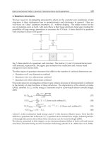
In these semitransparent layers, complex radiative phenomena occur. Indeed, the
multiplicity of layers causes complex reflection phenomena in the semitransparent medium.
This is shown in Fig 4. A ray of light that reach the surface of a layer of material will be
decomposed into three fluxes: absorbed, reflected and transmitted to deeper layer.

Solar
irradiance E
τ
α
ρ
Layer 1
Layer 2
Layer N
Transmitted
flow
Reflected
flow
Absorbed
flow

Fig. 4. Section view of the multiple reflections phenomena in a semi-transparent multilayer

material
Solar Collectors and Panels, Theory and Applications

414
Furthermore, another feature of the system is that it may contain air or water gaps. These air
gaps may be contained in the wall where the panel is installed or between the wall and the
photovoltaic panel (as in the case of Trombe walls or on some photovoltaic roofs). The
blades of water are present in hybrid PV systems. These layers of fluid are complex to
model, and are host of phenomena due to different ventilation or fluid circulation system
integration in the building. They may be influenced by conditions outside the system (such
as wind in the case of opened air gaps in roof installations).
3.2 Thermal phenomena and assumptions
The walls are modelled layer by layer. The goal is to find the energy transfer across the solar
system and its coupling with the building, it is not necessary to model finely phenomena. In
addition, the coupling of the wall model with the PV will be done with an existing code,
named ISOLAB (Miranville, 2003). This code models each type of walls in the same manner,
by reducing the thermal problem at the scale of the material layer.
ISOLAB is a building simulation code able to predict the heat and mass transfer in buildings
according to a nodal 1D description of the building and its corresponding thermo-physical
and geometrical parameters. The resolution is based on a finite difference numeric scheme
and the system of differential equations, written in a matrix form, is solved numerically for
each time step.
In the version of ISOLAB that was used as the basis for this work, the walls are described by
using heat balance equation. This equation is discretized by finite difference method
dynamically according to a nodal 1D description in the thickness of each wall.
The heat transfer equation takes classically into account the conduction phenomena in
different layers. It is to be noticed that the phenomena occurring in convective fluid layers
and radiative semitransparent layers must be described specifically.
Regarding the fluid layers, the choice was made to use empirical models. These models can
characterize the convective heat flux by determining the coefficient of convective heat

exchange between the fluid and the considered wall. This coefficient will depend on the
flow regime in the fluid layer and the temperature of the fluid. Several models have been
chosen to perform the tests; they were chosen to meet the most technical configurations of
the panel (Bigot, 2009). Note that the chosen models are not necessarily the most appropriate
in some cases. The goal here is to test the ability of these models to describe our system. It
will be necessary in the future to choose other models as appropriate, and to validate them.
These models were implemented directly in the PV model code. They are chosen
automatically by the program as needed (cavity vertical, inclined, horizontal, or depending
on the configuration of the air layer in terms of opening to the outside, and thus ventilation).
To model the radiative phenomena in the semitransparent medium, the model chosen
follows the "ray tracing" method. It is presented in the next section.
3.3 Derivation of the problem
The « ray tracing » method is a model that can describe radiative exchanges in
semitransparent mediums. In this work, the model was inspired of Robert Siegel works
(Siegel, 1992). This model consists on a net radiative balance of fluxes at each layer of
material. As its name suggests, a ray of light will be followed and dispatched every time it
will meet a new material surface (see Fig 4). With each new surface it encounters, the ray
will be divided into three parts until meeting an opaque layer: the flux absorbed by the layer
Thermal Performance of Photovoltaic Systems Integrated in Buildings

415
encountered, the flux transmitted through this layer, and the flux reflected by this layer to
the layer where the ray comes from. These phenomena are reproduced until encounter an
opaque layer (the layer N where τ > 0 on Fig. 4).
A system describing radiative flux exchanges can be defined for such a problem:
Φ
abs
(i,1,j) is the flow absorbed by the layer i at the iteration j on its exterior face (Φ
abs
(i,2,j)

corresponds to the inside); Φ
trans
(i→k,j) is the flux transmitted on the layer k by the layer i in
the iteration j, and Φ
ref
(i→k,j) is the reflected flux by the layer i on the layer k for the
iteration j. In the below relations, the indicated physical parameters are the following:
α
i
: absorption coefficient of the layer i
τ
i
: transmission coefficient of the layer i
ρ
i
: reflectivity coefficient of the layer i
ε
i
: emissivity coefficient of the layer i
F
pe
: view factor between the panel and the environment
F
pi
: view factor between layers i and j
E : incident shortwave radiation
T
i
: temperature of the layer i
Φ

abs
: absorbed radiation flux
Φ
trans
: transmitted radiation flux
Φ
ref
: reflected radiation flux
In terms of equations, the physical phenomenon can be described as indicated below :
•
Initial condition:
(
)
1
1,1,1
abs
p
e
ES F
α
Φ=⋅⋅⋅
(
)
112
12,1
trans
ES F
τ
Φ→=⋅⋅⋅
(

)
4
111,
1,1
trans N N N N
NN STF
εσ
+++
Φ+→=⋅⋅⋅⋅
•
Boundary conditions: for 2 ≤ j ≤ I:
()()()()
(
)
121
1,2, 1, 1,2 2 1, 1 2 1, 1
abs abs ref trans
jj j j
F
α
Φ=Φ−+Φ→−+Φ→−⋅⋅

(
)
1,0
trans
NNjΦ+→= ;
(
)
12, 0

trans
j
Φ
→=;
(
)
12, 0
ref
j
Φ
→=
()( )
()
(
)
11,
1, 1,1 1,1
re
f
trans re
f
NNN
NNj NNj NNJ F
ρ
++
Φ+→=Φ →+−+Φ→+−⋅⋅
•
System description: for 2 ≤ j ≤ I and 2 ≤ i ≤ N:
()()()()
(

)
1,
,1, , 1,1 1 , 1 1 , 1
abs abs re
f
trans i i i
i j ij i ij i ij F
α
−
Φ=Φ−+Φ−→−+Φ−→−⋅⋅
() ( ) ( ) ( )
(
)
1,
,2, , 1,2 1 , 1 1 , 1
abs abs re
f
trans i i i
ij ij i ij i ij F
α
+
Φ=Φ−+Φ+→−+Φ+→−⋅⋅

(
)
(
)
(
)
1,

1, 1 , 1
re
f
trans i i i
ii j i ij F
ρ
−
Φ→−=Φ −→−⋅⋅
(
)
(
)
(
)
1,
1, 1 , 1
re
f
trans i i i
ii j i ij F
ρ
+
Φ→+=Φ +→−⋅⋅
()( )( )
(
)
,1
1, 1 , 1 1 , 1
trans trans re
f

iii
ii j i ij i ij F
τ
−
Φ→−=Φ+→−+Φ+→−⋅⋅
()()()
(
)
,1
1, 1 , 1 1 , 1
trans trans re
f
iii
ii j i ij i ij F
τ
+
Φ→+=Φ−→−+Φ−→−⋅⋅
The absorbed flux by the layer situated after the PV system and the absorbed flux by each
layer are known:
()
()
1,1
1
1,1 1,
jI
abs N N N trans
j
NF NNj
α
=

++
=
Φ+=⋅ ⋅Φ →+
∑

Solar Collectors and Panels, Theory and Applications

416
()
1
(,1) ,,1
jI
abs abs
j
iij
=
=
Φ=Φ
∑

()
1
(,2) , ,2
jI
abs abs
j
iij
=
=
Φ=Φ

∑

Iterations can be stopped when the residual energy of the system is lower than a threshold
value (
erreur):
() ()
()
() ()
()
11
,, ,1,1
iN iN
trans ref trans ref
ii
ij ij ij ij erreur
==
==
Φ+Φ−Φ−+Φ−≤
∑∑

The integration of the PV module to the building simulation is done according to the
synoptic of Fig. 5. Once the thermal model of the considered building without PV panels is
generated, a test is done in order to detect the inclusion of PV panels; if PV panels are
detected, the PV module generates the corresponding system of equations and solves the
whole model. Results can then be analysed.

PV module
(generation of the PV matrix system
and assembly with the previous
thermal one)

Meteorological
data
Building physical and
structural description
Thermal model
Results (thermal field)
PV panel
included ?

Fig. 5. Integration of the PV calculation module to the existing ISOLAB code.
3.4 Numerical resolution
By discretizing the heat equation below as described above, we obtain a system describing
the evolution of the temperature in each building wall. This system of equations can be
written in matrix form to facilitate its handling and resolution.
2
2
1TT
P
at
x
∂∂
=
⋅−
∂
∂
where
p
a
C
λ

ρ
=
⋅

In the case where the material is a semi-transparent layer, P is the volumic heat power
absorbed by the semi-transparent layer. P is null in other cases.
Thermal Performance of Photovoltaic Systems Integrated in Buildings

417
We solve this equation by discretizing with a finite difference method. Each layer of material
is cut in many nodes. Three types of equations are obtained:
•
A first for nodes inside the layer:
1
111
1
12
c
tt tt
ccc
ccc
ttt
TT TTP
τττ
+
+++
−
⎛⎞
ΔΔΔ
=

−⋅ ++⋅ −⋅ +
⎜⎟
⎝⎠

•
A second for nodes on extremity of the wall or near a fluid layer (c is the number of the
node in the wall):
11
1
22
12
ttt
cccinc
ccc
Ttt
TTT
C
ϕ
ττ
++
−
⎛⎞
ΔΔΔ
=+⋅ ⋅−⋅−⋅
⎜⎟
⎝⎠

•
A third for nodes of the surface between two conductive materials:
1

11
11
11
tt t
cc
cc c
cc cc
kk
TT T
kk kk
+
++
+
−
++
=⋅+⋅
++

Where:
c
c
c
C
k
τ
= ;
c
cpc
CCx
ρ

=
⋅⋅Δ;
c
c
k
x
λ
=
Δ

For surface node temperatures, the φ
inc
corresponds to the sum of convective and radiative
exchange fluxes.
These equations are applied to all nodes of the building system, and we obtain an equation
system that describes the evolution of each temperature. It can be expressed in a numeric
form by the following matrix equation:
[][] [][]
1tt
ie
AT AT B
+
⋅
=⋅ +
Matrixes [A]
i
and [A]
e
describe the composition of the various materials constituting the
building, while [B] corresponds to outside or internal solicitations of the system. Matrixes

[T]
t
and [T]
t+1
contain all nodes temperatures of all walls.
Finally, a matrix system is obtained that describes the temperature evolution of the PV wall.
It is included like a traditional wall by ISOLAB to the matrix building system. Function of
the surfaces, the PV wall is partly or totally substituted to the wall where the PV panel is
installed.
4. Experimentation of BIPV
4.1 A dedicated experimental platform
In order to apply the preceding combined methodology, a dedicated experimental platform
was set up, in field environment. It is indeed very important to be able to determine the
physical behaviour of the whole building equipped with the BIPV or the BAPV, under realistic
conditions. For this, the experimental platform includes several cells, facing north, and fully
instrumented. A meteorological station is also integrated, to allow the measurement of the
climatic conditions of the location. The cells are of two types. A large scale test cell, named
LGI, is used to represent typical conditions of a real building and its thermal response. Four
other cells (ISOTEST cells) are installed on the platform, reduced size and dedicated to the
Solar Collectors and Panels, Theory and Applications

418
simultaneous comparison of different types of walls installed on buildings. An overview of the
platform is presented on fig 6 and the two types of cells are illustrated on fig 7.


Fig. 6 & 7. The experimental platform and the test cells
The study undertaken here is made with ISOTEST test cells in order to compare directly the
cases between the buildings which are equipped with a PV panel and those which are not
(see fig 8 and 9). These experimental cells have indeed been set up to allow a comparison

between the several types of roof components, all in the same conditions. Each of them is
equipped with a specific roof component and is fully instrumented to allow the physical
observation of the energetic behaviour. It has an interior volume of about 1m
3
and is
conceived from a modular structure, which means that with the same cell we can study
different configurations and phenomena. This is why the walls are movable. It constitutes a
basis for the thermal studies of building components, with the advantage of flexibility and
easy-to-use, especially when several products must be tested. It is installed in-situ, which
allows us a better observation of the actual behaviour of the cell. Thanks to this method, we
are able to know the temperature of each part of the system in different configurations but
in the same environmental conditions. Comparisons between the test cells have been made.
Before this, a calibration step has been done to make sure that the four cells had the same
thermal behaviour.


Fig. 8. Current aerial view of Isotest Cells
Thermal Performance of Photovoltaic Systems Integrated in Buildings

419



Fig. 9. Photography of Isotest cell without and with PV panel.
4.2 Data acquisition sensors and errors
The data measured in this experiment are inside surface temperatures of walls and roof, air
temperatures, and heat flux through each roofs (see fig 10). The global error of these
measurement equipments (sensors and data acquisition system) is about one degree Celsius
(±1°C) for the temperature and ±10% for the heat flux (Miranville, 2002). The last study
made with this equipment dating for one year, it was necessary to calibrate the equipment.

This was done by running a calibration procedure consisting in determining the calibration
coefficient allowing the correct inter-comparison of the response of the cells.


Fig. 10. Sensors installation in the roof wall.
5. Validation
5.1 Overview
Building simulation codes are useful to point out the energetic behaviour of a building as a
function of given inputs. The steps involved in this process depend on a mathematical
Solar Collectors and Panels, Theory and Applications

420
model, which is considered a global model because it involves several so-called elementary
models (conductive, convective, radiative, etc.). Therefore the validation procedure will
involve verifying not only the elementary models, but also their coupling, as the building
model can be seen as the coupling of a given combination of elementary models.
For several years a common international validation methodology has been developed,
which, among others, has led to Anglo-French cooperation. This latter brought to fruition a
common validation methodology, involving two test categories, as indicated in table 2.

Verification of the basic theory
Verification of good numerical
behaviour
Comparison of software
Analytic verification of elementary
models
‘Pre-Tests’
Parametric sensitivity analysis
Empirical validation
‘Post-Tests’

Table 2. Global validation methodology
The first, generally called ‘a priori’ or ‘pre-‘ tests, involves the verification of the
programming code, from the under-lying theory of the elementary models, to software
comparisons, and finally to analytic verifications. The objective is to ensure the correct
implementation of the elementary models and the correct representation of their coupling at
the level of the global model.
This important step of validation justifies the development of dedicated software tools, such
as the BESTEST procedure (Judkoff et al., 1995). This latter is essentially based on the
comparison between the programming code predictions with so-called reference software
results, for a range of different configurations. As a result it includes aspects of verification
of correct numerical behaviour and of cross-software comparison, and allows us to compare
the program to analogue tools. If the results compare well with those found during this
procedure, the programming code is considered acceptable.
The second part of the validation methodology, known as the ‘a posteriori’ or ‘post-’tests,
involves two main steps, the parametric sensitivity analysis and, most important, the
empirical validation. This second step is fundamental, because it compares the program’s
predictions with the physical reality of the phenomena, using measurements. It therefore
requires an experiment to be set-up, with the aim of obtaining high quality measurements.
The sensitivity analysis of the model consists of finding the set of parameters with most
influence on a particular output. It is also used when seeking the cause of any difference
between the model and measurements, and allows us to focus this search on a restricted set
of parameters, which control the considered output.
Further, the empirical validation methodology is a function of the given objective and of the
type of model under consideration; in our case, the empirical validation must allow us to
demonstrate the correct thermal behaviour of the building envelope, in particular at the
level of the complex wall including a PV panel.
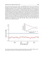
5.3 Empirical validation
In order to improve the PV model, a comparison has been made between measurements and
simulation data (see fig. 11) for the case of the PV panel with a confined air layer. In
Thermal Performance of Photovoltaic Systems Integrated in Buildings

421
previous articles, the ISOLAB code has already been validated in many cases by
comparisons with other building simulation codes, as well as experimental validations. This
comparisons can show advantages and disadvantages of the model. In figures presented
below, the main temperatures are compared for the previous cell.


Fig. 11. Temperatures of the PV installation with a confined air layer.
For the temperatures obtained for the body of the cell, a good agreement is obtained, the
average difference of temperature being weak, of the order of 1°C. Nevertheless Figure 11
shows, although the PV model has a good dynamic behaviour in the case of a confined air
layer, noticeable differences between the model and the reality of measurements. These
differences can be related to:
•
Thermo-physical properties (conduction, thermal capacity, transmitivity, absorptivity )
of each PV panel material, which are not exactly known. Industrials did not give details
of those properties in order to protect their copyright.
•
The precision of the radiative model (of PV panels) or convective model (of air layer) in
the PV modelling.
To give elements of answers for these differences between predictions and measurements, a
sensitivity analysis was made, as explained in the following paragraph.
5.4 Sensitivity analysis
The sensitivity analysis consists in performing several simulation runs by oscillating each
parameter according to a sinusoid over its range of interest. Analyzing the spectrum
(Fourier transform or power spectral density) of the output, identification of the most
influential factors can be easily derived (Mara, 2000); (Mara et al., 2000); (Mara, 2002).
Solar Collectors and Panels, Theory and Applications

422

Fig. 12. Procedure of sensitivity analysis.
The proposed FAST method (Fast Fourier Amplitude Transform) uses a sinusoidal sampling
of parameters around their base value, each parameter having its own frequency, the
variation being applied to a simulation on the other as shown in fig. 12. Thus, the process is
analogous to the use of an experimental design where the parameters are varied in each test
according to a predetermined pattern, so to sweep the best surface model response.
The sensitivity analysis is composed of three steps:
•
The first step that put in evidence the most influential parameters, shown on the figure
13 (Fourier spectrum). For each frequency that corresponds to each parameter it can be
shown if it has an effect on the outputs.
•
The second step presents principal effects of each parameter on the outputs. It
represents the linear effect of each parameter.
•
The third step presents non linear effects of parameters on the outputs. Contrary to
principal effects, it takes into account the effect of a parameter in interaction with other
parameters.
In this study, only principal effects are presented, because non linear effects are negligible
compare to principal effects (the maximum interactional effect is about 0.1°C).
The sensitivity analysis was run with a thermal simulation of the building during two days
in January 2009. A variation of 10% was applied to all parameters contained in the building
and PV panel descriptions.
In a First run, the inside air temperature of the building was chosen has the output. Results
show that several parameters of the PV thermal model are influential on this temperature
(see fig. 13 an fig. 14).
The fig. 13 shows the Fourier spectrum, and also parameters of influence. Fig. 14 shows
parameter effects, and the magnitude of influence of each parameter, described by a

frequency number (see Table 3).
Thermal Performance of Photovoltaic Systems Integrated in Buildings

423

Fig. 13. Fourier spectrum of the sensitivity analysis for the inside air temperature of the
building

Table 3. Designation of influential parameters of PV model on temperatures of the building
Because the inconsistency seems to come from the modelling of the PV system (ie the assembly
of the PV panel and the roof wall), the sensitivity analysis was made for temperatures of all
layers of the PV panel system and for the building inside air temperature.
The analysis emphases thermo-physical parameters like thermal conductivity, heat capacity
or transmitivity. These results show that three types of thermal transfer must be described
more precisely or in a different way, because they are very influential on the air temperature
inside the building:
•
the transmission of solar irradiation through the semi-transparent system in the PV
panel, and the absorption of solar irradiation by the first opaque layer,
•
the thermal conduction through all opaque layers after semi-transparent complex system,
•
the convection transfer in air gaps in the PV complex wall (like the air gap besides the
PV panel).
Solar Collectors and Panels, Theory and Applications

424
Furthermore, optical properties of semi transparent layers and characterization of the flow
in inclined air gaps are not easy to visualize or describe. These phenomena have been
described by commonly accepted parameters, but it is not sure it corresponds exactly to

reality. So these results seem quite realistic.


Fig. 14. Principal effect of sensitivity analysis of the inside air temperature of building
Focusing the sensitivity analysis on different layers of the PV complex wall, it can be shown
that the most influential parameters are those presented above. Basically, it depends on the
transmitivity of all semi-transparent layers through which solar irradiation is transferred, on
the conductivity of all opaque layers, and on convective heat transfer coefficients of air gaps
of the system.
The next step consists in optimizing parameters of the thermal modelling, as it is introduced
as following.
5.5 Optimization
The optimization is the step where the model can be improved and validated. It can be
made by using optimization algorithms. In this chapter, we present the use of a free
optimization program called GENOPT (Wetter, 2001). This program was set up to allow
anyone to use it with his own simulation code. It has been coupled with many building
simulation codes like EnergyPlus, TRNSYS, SPARK, IDA-ICE or DOE-2.
GENOPT make the optimization by running simulations of the studied code. It changes
values of parameters in the inputs of the program and notes the variation induced on the
outputs. As it is shown on fig. 14, it needs only three files to run: the input file, the output
file and also the program it has to run. Furthermore, it needs information about the
optimization algorithm, studied parameters and the cost function.
Thermal Performance of Photovoltaic Systems Integrated in Buildings

425

Fig. 14. Synoptic of the coupling of the building simulation code ISOLAB with GENOPT.
To use GENOPT as it is presented in fig. 14, it is necessary to create a complete standalone
simulation code; i.e. a program that does not need the human intervention to run a
simulation. This step is particularly complex in our case, because ISOLAB was made to be

used with the presence of a human kind in all steps of the simulation process.
The interfacing between GENOPT and ISOLAB is in the last test phase. The next step will be
the optimisation procedure of the PV system, with the precise determination of the best set
of parameters, including conductive, convective and radiative aspects.
Finally, the corroboration of the optimised model will terminate the validation procedure,
and allow the generalised use of the model for precise building design.
6. Conclusion
6.1 Thermal Performance of BIPV
The review on BIPV has demonstrated that not only a unique physical model exists, capable
of predicting the thermal evolution of the building envelope with the influence of
photovoltaic systems in various configurations (integrated-façade, integrated-roof,
integrated-glazing, etc.). This chapter has presented a semi-detailed model of a fully coupled
PV model, integrated in a building simulation code. The model was used to predict the
temperature field in the complex wall constituted by the PV system and its support wall. A
global validation procedure (including a sensitivity analysis) has been conducted to
determine the precision level of the results and has shown that the performance of the BIPV
was greatly dependant on the radiative heat transfer within the semi-transparent layers and
the convective heat transfer in the fluid layers. Moreover, the opaque layer included in the
system plays also, according to its radiative properties, an important role on the whole
behaviour of the system. The main problem is the modelling of convective air-gaps, in
which coupled heat transfers arise, the intensity of the coupling being function of the
configurations of the photovoltaic installation (angles, thickness and distribution of air
spaces in the panel, etc).
Files locatio
n
Algorithm
p
arameters
Building code
informatio

n
Input file
GENOPT
ISOLAB
Building
descri
p
tio
n
Temperature
field
Optimized
model
Solar Collectors and Panels, Theory and Applications

426
6.2 Model validity
Experimentation data was compared to simulation data. This comparison shows that the
thermal model has a good dynamic. However, there are some fairly large differences in
amplitude for temperatures of the PV complex wall. To provide some answers to this
problem, a sensitivity analysis was run and brought to light the most important parameters
on the behaviour of the system. An optimisation procedure is planned, to determine the best
set of parameters to lead to the best performance of the BIPV. Adjusting these parameters
will considerably reduce the observed difference between measurements and predictions,
and lead to the validation of the building envelope model. This important step is in progress
and will be presented in future works.
6.3 Coupling with PCMs
One possible perspective is to couple the BIPV with MCPs (phase change materials). These
are materials capable of changing of physical state within wide ranges of temperatures
according to desired applications (building insulation, passive cooling, thermal energy

storage, textile industry, etc.).
These materials have the ability to store or to release a large amount of energy as latent heat
during phase change liquid-solid. They can be classified into three broad categories:
•
The MCP organic (paraffin and fatty acid)
•
The MCP inorganic (hydrated salt)
•
The MCP eutectic (organic-organic, organic-inorganic, inorganic-inorganic)
The choice of MCPs is based on a number of factors such as latent and sensible heat, thermal
conductivity in liquid and solid phases but also the impact on the overall thermal
performance of the entire system and its cost.
The coupling of the PCM with BIPV could be considered as liquid-solid phase change to
reduce the temperature rise within the BIPV but also increase their performance and their
life.
6.4 Toward zero net energy buildings
The building simulation code used for this study henceforth includes a generic model, fully
coupled, for the complete modelling of the integration of PV panels in buildings. More and
more used in the world, as a means of electricity production using renewable energy, PV
systems are of great potential and are subject to numerous research programs. Their
inclusion in building envelopes opens the way for zero net energy constructions, whose
potential in terms of energy consumption and reduction of global warming is more and
more recognised. In a near future, with constant developments and improvements, our
building simulation code will be able to predict the energetic behaviourof zero net energy
buildings and thus the evaluation and optimisation of their performances.
7. References
Bazilian M. D., Prasad D. Thermal and electrical performance monitoring of a combined
BIPV array and modular heat recovery system. In: ISES Solar World Congress
Adelaide, Australia, 2001
Bazilian M. D. Australia’s first BiPV/thermal test facility (an ACRE funded research project).

In: PV in Europe, Rome, 2002
Thermal Performance of Photovoltaic Systems Integrated in Buildings

427
Bigot D., Miranville F., Fakra A., H. Boyer H. (2009). A nodal thermal model for photovoltaic
systems: impact on building temperature field elements of validation for humid
climatic conditions. Energy and Buildings, Vol. 41, June 2009, 1117-1126
Cherruault J., Wheldon A. (2001). Evaluation of a BIPV roof, designed for expandability and
using coloured cells. DTI Substainable Energy Programmes. DTI Pub/URN
01/1395, ETSU S/P2/00297/REP, 80 p. University of Reading, Renewable Energy
Helpline
Chow T., He W., Chan A. L. S., Fong K. F., Lin Z., Li J. (2008). Computer modelling and
experimental validation of a building-integrated photovoltaic and water heating
system. Applied Thermal Engineering, Vol. 28, October 2007, 1356-1364
Fung T. Y., Yang H. (2008). Study on thermal performance of semi-transparent building-
integrated photovoltaic glazing’s. Energy and Buildings, Vol. 40, February 2007,
341-350
Guiavarch A., Peuportier B. (2006). Photovoltaic collectors efficiency according to their
integration in buildings. Solar Energy, January 2006, Vol. 80 issue 1, 65–77
Jie J., Hua Y., Wei H., Gang P., Jianping L., Bin, J. (2007). Modeling of a novel Trombe wall
with PV cells. Building and Environment, Vol. 42, January 2006, 1544-1552
Jiménez M. J., Madsen H., Bloem J., Dammann B. (2008). Estimation of non-linear
continuous time models for the heat exchange dynamics of building integrated
photovoltaic modules. Energy and Buildings, Vol. 40, February 2007, 157-167
Judkoff R. D., Neymark J. S. A Procedure for Testing the Ability of Whole Building Energy
Simulation Programs to Thermally Model the Building Fabric. Journal of Solar
Energy Engineering, Transactions of ASME, Volume 117, pp. 7-15, 1995
Kondratenko IV. Urban retrofit building integrated photovoltaics [BIPV] in Schotland, with
particular reference to double skin facades. PhD thesis, University of Glasgow, 2003
Kropf S. PV/T Schiefer, Optimierung der Energieeffizienz von Gebaüden durch

gegenseitige Erga¨nzung von Simulation und Messung am Beispiel der Hinterlu¨
ftung geba¨ udeintegrierter Photovoltaik. PhD report, ETH Zurich, 2003
Mara T., Boyer H., Garde F. and Adelard L. Présentation et Application d'une Technique
d'Analyse de Sensibilité Paramétrique en Thermique du Bâtiment, Société Française
de Thermique SFT 2000, Lyon, France. p.795-800. 2000.
Mara T., Garde F., Boyer H., Mamode M., Empirical validation of the thermal model of a
passive solar test cell. Energy and Buildings. Vol.1320, p.1 - 11. 2000.
Mara T., Boyer H., Garde F. Parametric Sensitivity Analysis of test cell thermal model using
spectral analysis. ASME Journal of Solar Energy Engineering. Vol.124, p.237 – 242.
(2002)
Mei L., Infield D. G., Gosttschalg R., Loveday D. L., Davies D., Berry M. (2009). Equilibrium
thermal characteristics of building integrated photovoltaic tiled roof. Solar Energy,
Vol. 83, July 2009, 1893-1901
Miranville F. Contribution à l’Etude des Parois Complexes en Physique du Bâtiment. Thesis.
University of La Reunion, La Reunion (France). 2002.
Miranville F., Boyer H., Mara T., Garde F. On the thermal behaviour of roof-mounted
radiant barriers under tropical and humid climatic conditions. Energy and
Buildings, Volume 35, Issue 10, November 2003, Pages 997-1008
Norme ISO-9869-1994, Isolation thermique – Elements de construction – Mesures in-situ de
la resistance thermique et de la transmittance thermique
Solar Collectors and Panels, Theory and Applications

428
Nynne F., Maria, J., Hans B., Henrik M. (2009). Modelling the heat dynamics building
integrated and ventilated photovoltaic modules. Energy and Buildings, Vol. 41,
May 2009, 1051-1057
Park K. E., Kang H. G., Kim H. I., Yu G. J., Kim J. T. (2010). Analysis of thermal and electrical
performance of semi – transparent photovoltaic module. Energy, Vol. 35, July 2009,
2681 – 2687
Siegel R. 1992. Thermal Radiation Heat Transfer. Hemisphere, Washington.

Skoplaski E., Palyvos J. A. (2009). Operating temperature of photovoltaic modules: Asurvey
of pertinent correlations. Renewable Energy, Vol. 34, june 2008, 23-29
Steven V. D., Benjamin F. (2010). Active thermal insulators: finite elements modelling and
parametric study of thermoelectric modules integrated into a double pane glazing
system. Energy and Buildings, Vol. 42, February 2010, 1156-1164
Tian W., Wang Y., Xie Y., Wu D., Zhu L., Ren J. (2007). Effect of building integrated
photovoltaic on microclimate of urban canopy layer. Building and Environment,
Vol. 42, February 2006, 1891-1901
Trinuruk P., Sorapipatana C., Chenvidhya D. (2009). Estimating operating cell temperature
of BIPV modules in Thailand. Renewable Energy, Vol. 34., February 2009, 2515-
2523
Wang Y., Tian W., Ren J., Zhu L., Wang Q. (2006). Influence of a building’s integrated-
photovoltaic on heating and cooling loads. Applied Energy, Vol. 83, December
2005, 989-1003
Wetter M. GENOPT - A generic optimization program. In R. Lamberts, C. O. R. Negrao, and
J. Hensen, editors, Proc. of the 7th IBPSA Conference, volume I, pages 601-608. Rio
de Janeiro, 2001.
Xu X., Dessel V. S. (2008). Evaluation of a prototype active building envelope window –
system. Energy and Buildings, Vol. 40, February 2007, 168-174
Zonda H. A. Combined PV-air collector as heat pump air preheater. Staffelstein, 2001
Zondag H. A. (2008). Flate-Plate PV-Thermal collectors and systems: A review. Renewable
and Sustainable Energy Reviews, Vol. 12, December 2005, 891-959
20
Working Fluid Selection for Low Temperature
Solar Thermal Power Generation with Two-stage
Collectors and Heat Storage Units
Pei Gang, Li Jing, Ji Jie

Department of Thermal Science and Energy Engineering, University of Science and
Technology of China, Jinzhai Road 96#, Hefei City, Anhui Province,

People’s Republic of China
1. Introduction
Organic Rankine Cycle (ORC) is named for its use of an organic, high molecular mass fluid
that boils at a lower temperature than the water. Among many well-proven technologies,
the ORC is one of the most favorable and promising ways for low-temperature applications.
In comparison to water, organic fluids are advantageous when the plant runs at low
temperature or low power. The ORC is scalable to smaller unit sizes and higher efficiencies
during cooler ambient temperatures, immune from freezing at cold winter nighttime
temperatures, and adaptable for conducting semi-attended or unattended operations [1].
Simpler and cheaper turbine can be used due to the limited volume ratio of organic fluid at
the turbine outlet and inlet [2]. In the case of a dry fluid, ORC can be employed at lower
temperatures without requiring superheating. This results in a practical increase in
efficiency over the use of the cycle with water as the working fluid [3]. ORC can be easily
modularized and utilized in conjunction with various heat sources. The success of the ORC
technology is reinforced by high technological maturity of majority of its components,
spurred by extensive use in refrigeration applications [4]. Moreover, electricity generation
near the point of use will lead to smaller-scale power plants, and thus the ORC is
particularly suitable for off-grid generation.
The selection of the working fluid is of key importance in ORC applications. This is because
the fluid must have not only thermophysical properties that match the application but also
adequate chemical stability at the desired working temperature. There are several optimal
characteristics of the working fluid:
1. Dry or isentropic fluid to avoid superheating at the turbine inlet, for the sake of an
acceptable cycle efficiency;
2. Chemical stability to prevent deteriorations and decomposition at operating
temperatures;
3. Non-fouling, non-corrosiveness, non-toxicity and non-flammability;
4. Good availability and low cost.
However, not all the desired general requirements can be satisfied in a practical ORC. In the
previous research, numerous theoretical and experimental studies have focused on ORC

fluid selection with special respect to thermodynamic properties. Hung et al. studied waste
Solar Collectors and Panels, Theory and Applications

430
heat recovery of ORC using dry fluids. The results revealed that irreversibility depended on
the type of heat source. Working fluid of the lowest irreversibility in recovering high-
temperature waste heat fails to perform favorably in recovering low-temperature waste heat
[5]. Liu et al. presented a performance analysis of ORC subjected to the influence of working
fluid. It was revealed that thermal efficiency for various working fluids is a weak function of
critical temperature [6]. Saleh et al. conducted a thermodynamic screening of 31 pure
component working fluids for ORC using Backone equation of state. It was suggested that
should the vapor leaving the turbine be superheated, an internal heat exchanger may be
employed [7]. Madhawa et al. presented a cost-effective optimum design criterion for ORC
utilizing low-temperature geothermal heat sources. Results indicated that ammonia
possesses minimum objective function because of a better heat transfer performance, but not
necessarily a maximum cycle efficiency [8]. Drescher et al. proposed a new heat transfer
configuration with two thermal oil cycles to avoid the constriction of the pinch point
between the organic fluid and thermal oil at the beginning of vaporization in biomass power
and heat plants. Based on the new design, the influence of working fluids was analyzed and
the family of alkyl benzenes showed highest efficiencies [9].
It should be noted that the majority of the previous research on ORC fluid selection was
concerned in fields of waste heat recovery, geothermal and biomass applications.
Integration of ORC and solar collectors has attracted limited attention. Wang et al. designed,
constructed, and tested a prototype low-temperature solar Rankine system. With a 1.73 kW
rolling-piston expander overall power generation efficiency is estimated at 4.2% or 3.2% for
evacuated or flat plate collectors (FPC) respectively [10]. Ormat supplied a 1 MW power
plant, based on ORC technology, to the new power facility of Arizona Public Service. It
represented the first parabolic trough plant constructed since 1991 [11].
This paper combines ORC with compound parabolic concentrator (CPC). The feasibility and
advantage of CPC application in solar thermal electric generation have been outlined [12, 13,

14]. In particular, FPCs are employed in series with CPC collectors. Three considerations
should be made to understand the advantage of two-stage collectors. First, although CPC
collectors offer relatively low overall heat loss when operated at high temperatures,
efficiency may be lower than that of FPCs in low temperature ranges. Reflectivity of CPC
reflectors and difference between the inner and outer diagram of the evacuated tube result
in lower intercept efficiency. Thus, overall collector efficiency may be improved when FPCs
are employed to preheat the working fluid prior to entering a field of higher-temperature
CPC collectors. Second, FPC can absorb energy originating from all directions above the
absorber (both beam and diffuse solar irradiance). Third, FPC currently costs less than CPC
collector. Part of the reason is that production of FPC is considerably larger. Many excellent
models of FPC are available commercially for solar designers [15]. Similarly, collector
efficiency may be improved when two-stage heat storage units are employed with phase
change material (PCM) of a lower melting point as the first stage, and PCM of a higher
melting point as the second stage. Details are provided in the sections below.
Due this innovative design the working fluid selection criteria are different from that for a
solo ORC or ORC plants in waste heat recovery, geothermal and biomass fields. The
collector efficiency will be influenced directly by the thermophysical properties of the
working fluid e.g. the enthalpy-temperature diagram in the isobaric heating process.
Furthermore, the optimal proportion of FPC area to overall collector area for the two-stage
collectors is determined by both the operation condition and selection of working fluid.
Working Fluid Selection for Low Temperature Solar Thermal Power Generation
with Two-stage Collectors and Heat Storage Units

431
The low-temperature solar thermal electric generation with two-stage collectors and heat
storage units is first designed. Subsequently, fundamentals of heat transfer and
thermodynamics are illustrated. A mathematical model is established and a numerical
simulation is carried out. Five widely or newly used fluids are considered in this study. The
influences of working fluids on heat collection, ORC and global electricity efficiency are
investigated. Performance comparison among R113, R123, R245fa, pentane and butane is

presented.
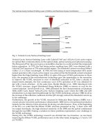
2. Design and fundamentals
Figure 1 presents the diagram of low-temperature solar thermal electric generation with two-
stage collectors and heat storage units. The system consists of FPC and CPC collectors, heat
storage, and ORC subsystem. FPCs offer the advantage of accepting high pressure without
leakage. The organic fluid flows through FPCs directly and is heated indirectly by CPC
collectors with the intermediate of conduction oil. The ORC subsystem consists of evaporator
(E), organic fluid/heat storage tank with PCM, turbine (T), generator (G), regenerator (R),
condenser, and pumps. The first-stage heat storage is filled with PCM (1), while the second
heat storage is filled with PCM (2). Melting point of PCM (1) is lower than that of PCM (2).


Fig. 1. Low-temperature solar thermal electric generation with two-stage collectors and heat
storage units
Solar Collectors and Panels, Theory and Applications

432
There are three basic modes of the low-temperature solar thermal electricity system in the
practical operating period. In Mode I, the system requires generation of electricity and
irradiation is available. In this mode, Valves 1, 2, 3, 4, and 5 are open. Pumps 1 and 3 are
running. Valves 11 and 12 may be open while Pump 2 may run to prevent superheating in
the evaporator when irradiation is strong. Flow direction of the organic fluid is illustrated
by arrows. Organic fluid is preheated in FPCs and subsequently vaporized in the evaporator
under high pressure. In the event that organic fluid is not totally vaporized, liquid will drop
into the fluid storage tank; it will not harm the turbine. Vapor flows into the turbine and
expands, exporting power in the process because of enthalpy drop. The outlet vapor is
cooled down in the regenerator and condensed to a liquid state in the condenser.
Meanwhile, the liquid is pressurized by Pump 1 and warmed in the regenerator.
Subsequently, organic fluid is sent back to the first stage collectors and is circulated. On the
use of Pump 2, the system can run steadily in a wide irradiation range. Without any

complicated controlling device, the process of heat storage or heat release can occur while
electricity is being generated.
In Mode II, the system does not require generation of electricity but irradiation is sound.
Valves 2, 8, 9, and 10 are open. Pumps 3 and 4 are running. The dashed lines in Fig.1
represent pipes for heat storage, with the exception of the line that passes through Valves 6
and 7. FPCs are connected with PCM (1) and CPC collectors are connected with PCM (2).
In Mode III, the system requires generation of electricity; however, irradiation is either
extremely weak or unavailable. Valves 1, 6, and 7 are open, and Pump 1 is running. Organic
fluid is preheated by the first-stage heat storage of PCM (1) and further heated by the
second-stage heat storage of PCM (2).
Mode I is described as the simultaneous processes of heat collection and power conversion
and is under special investigation in this work.
3. Working fluid properties
The ORC fluid can be classified into three categories according to the temperature-entropy
()Ts− diagrams. It is noteworthy that for some kinds of fluids, the derivative of
temperature with respect to entropy on the saturation vapor curve may change from
positive value to negative value, e.g.
dT
ds
of R123 on the saturation vapor curve is positive
when
T is smaller than 150°C while negative at higher temperature ranges. In this case, dry
fluids are generally named for the positive
dT
ds
in practical operation temperature range
from the cold side to the hot side. And wet fluids would have negative
dT
ds
on the saturation

vapor curve. Meanwhile, isentropic fluids have approximately infinite value of
dT
ds
(nearly
vertical curve).
The working fluids of dry or isentropic type are more appropriate for ORC systems. The
reason is that dry or isentropic fluids are superheated after isentropic expansion, thereby
eliminating the concerns of impingement of liquid droplets on the turbine blades and
making the superheated apparatus unnecessary [6]. Based on this consideration, five dry
fluids are selected in the analysis. They are R113, R123, R245fa, pentane and butane. Some of
properties of these fluids are listed in table 1. The optimal FPC proportion and the overall
collector efficiency are related to the latent heat and heat capacity in saturation liquid states
as discussed in Section 5.3.
Working Fluid Selection for Low Temperature Solar Thermal Power Generation
with Two-stage Collectors and Heat Storage Units

433
R123 R113 R245fa pentane butane
Critical pressure /Mpa 3.66 3.39 3.65 3.37 3.79
Critical temperature /°C 183.7 214.1 154.1 196.6 152.0
Boiling point /°C 27.8 47.5 15.1 36.1 -0.5
Latent heat, 120/°C kJ/kg 120.52 116.61 111.77 271.13 213.35
Heat capacity in saturation
liquid state, kJ/(kg·°C)
1.20 1.04 1.78 2.91 3.52
Table 1. Thermodynamic properties of the working fluids
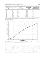
4. Thermodynamics and heat transfer
4.1 Calculation of thermodynamic cycle
Figure 2 presents the scheme of thermodynamic cycle of a typical dry fluid. Point 1
illustrates the state of fluid at the condenser outlet; Point 2 at the Pump 1 outlet; Point 2′ at

the regenerator outlet; Point 3 at the FPC collectors outlet; Point 4 at the evaporator outlet
(on the normal condition of irradiation); and Point 5 at the turbine outlet. The points being
referred to in Fig. 2 are placed in Fig. 1 with circles outside the numbers (with the exception
of 2′). The reversible process of pressurization or expansion are described by 2 s or 5s
respectively. Formulas for heat transfer and power conversion are developed below.
Enthalpy at Point 2′ is calculated by the following:

62
2256( )
[]
TT r
hhhh
ε
′
=
=
+− ⋅
(1)
Where
r
ε
is the regenerator efficiency. Enthalpy at Point 6 is assigned by assuming
62
TT= .
Total heat transferred to organic fluid from the collectors is calculated by the following:

42
Qh h
′
=−

(2)
Power generated by the turbine (Eq.3) and that consumed by Pump 1 (Eq.4) are calculated
by the following:

45
45
()
()
t
ts
Whh
hh
ε
=−
=−
(3)

,1 2 1
12 1
()
()/
p
p
Whh
vp p
η
=−
=−
(4)
Meanwhile, net power is calculated by the following:

,1 ,2orc t
gp p
WW WW
ε
=
⋅− −
(5)
In case the negative effect of Pump 2 is considered, calculation of required power
,2
p
W
is
presented in the following section. Practical ORC efficiency is calculated by the following:

orc
orc
W
Q
η
=
(6)
Solar Collectors and Panels, Theory and Applications

434

Fig. 2. Thermodynamic cycle of a typical dry fluid
4.2 Equations developed for total thermal efficiency of the collector system
The FPC or CPC collector module available in the market has an effective area of
approximately 2.0

2
m . Its thermal efficiency can be expressed by the following equation:

2
0
()()
aa
AB
TT TT
GG
ηη
=− − − −
(7)
Solar thermal electric generation system may demand tens or hundreds of collectors in
series, and the temperature differences between neighboring collectors will be small. Thus, it
is reasonable to assume the following: 1) the average operating temperature of the collector
changes continuously from one module to anther module; and 2) the function of the
simulated area of the collector system is integrable.
With inlet temperature T
i
and outlet temperature T
o
, the required solar collection area is
obtained by the following [12]:

()
()
T
o
p

T
i
mC T
SdT
TG
η
=
∫
(8)
Temperature of conduction oil in the CPC changes within a small range. This is discussed
further in Section 5.2. Heat capacity can be well approximated by the following [16]:


,0 0
() ( )
pp
CT C T T
α
=
+−
(9)
In the case of FPCs, organic fluid is preheated in low temperature ranges and the first-order
approximation of heat capacity can be used as well.
Working Fluid Selection for Low Temperature Solar Thermal Power Generation
with Two-stage Collectors and Heat Storage Units

435
With
1
/cAG= ,

2
/cBG
=
, the collection area according to Eqs. 8 and 9 is integrated by the
following:

12
,1 ,2
221 1 2
( )ln ( )ln
()
oa ia
pa pa
ia oa
TT TT
m
SC C
cG T T T T
θθ
αθ αθ
θθ θ θ
⎡
⎤
−− −+
=+++
⎢
⎥
−−− −+
⎣
⎦

(10)
where
1
θ
and
2
θ
are the arithmetical solutions of the following equations (
12
0, 0
θ
θ
<
> ).

2
12
0
o
cc
ηθθ
−
−=
. (11)

,,0 0
()
pa p a
CC TT
α

=
+− (12)
Subsequently, total thermal efficiency of the collector system is calculated using the
following:

()
T
o
cp
T
i
m
CTdT
GS
η
=
∫
(13)
Combining Eq.13 with Eqs.9 and 10, the following is obtained:

22 1 ,0 0
12
,1 ,2
12
()[()0.5()( 2)]
()
( )ln ( )ln
poi oioi
c
oa ia

pa pa
ia oa
c C TT TTTT T
TT TT
CC
TT TT
θθ α
η
θθ
αθ αθ
θθ
−−+−+−
=
−− −+
+++
−− −+
(14)

Effect of c
1
is expressed by Eq.11 There are two inlet temperatures, as well as two outlet
temperatures in the two-stage collectors. Total collector efficiency is calculated by the
following:

12
12
c
FPC CPC
QHH
HH

GS
η
ηη
Δ+Δ
==
ΔΔ
+
(15)
where
FPC
η
or
CPC
η
is the first- or second-stage collector efficiency, and
1
H
Δ
or
2
HΔ is the
enthalpy increment of working fluid in the first- or second-stage collectors. The value of
,0
p
C
or
α
or collector heat loss coefficient varies when the fluid or the collector is different.
4.3 Heat transfer between conduction oil and working fluid
Thermal efficiency of FPCs can be calculated directly by the inlet and outlet temperatures of

working fluid, according to Eq.14. On the other hand, thermal efficiency of CPC collectors is
determined by the heat transfer process in the evaporator. The temperature relationship
between working fluid and conduction oil must be established.

This section focuses on heat transfer in the evaporator, and the developed equations can
easily be extended to the case of the condenser. Counter-current concentric tubes are
adopted, and the parameters are listed in Table 2.