Urban Transport and Hybrid Vehiclesedited Part 9 ppt
Bạn đang xem bản rút gọn của tài liệu. Xem và tải ngay bản đầy đủ của tài liệu tại đây (1.23 MB, 20 trang )
Analysis of the Regenerative Braking System
for a Hybrid Electric Vehicle using Electro-Mechanical Brakes
153
2. HEV powertrain modeling
Figure 3 shows the structure of the HEV investigated in this paper. The power source of this
HEV is a 1.4 liter internal combustion engine and a 24 kW electric motor connected to one of
the axes. The transmission and braking system are an Automated Manual Transmission
(AMT) and an EMB system with pedal stroke simulator, respectively. EMB supplies braking
torque to all four wheels independently, and the pedal stroke simulator mimics the feeling
of the brake pedal on the driver’s foot.
Fig. 3. Configuration of HEV braking control system
The vehicle controller determines the regenerative braking torque and the EMB torque
according to various driving conditions such as driver input, vehicle velocity, battery State
of Charge (SOC), and motor characteristics. The Motor Control Unit (MCU) controls the
regenerative braking torque through command signals from the vehicle controller. The
Brake Control Unit (BCU) receives input from the driver via an electronic pedal and stroke
simulator, then transmits the braking command signals to each EMB. This is determined by
the regenerative braking control algorithm from the value of remaining braking torque
minus the regenerative braking torque. The braking friction torque is generated when the
EMB in each wheel creates a suitable braking torque for the motor; the torque is then
transmitted through the gear mechanism to the caliper (Ahn et al., 2009).
2.1 Engine
Figure 4 shows the engine characteristic map used in this paper. The complicated
characteristics of this engine are due to many factors, such as fuel injection time, ignition
time, and combustion process. This study uses an approximated model along with the
steady state characteristic curve shown in Figure 4.
The dynamics of the engine can be expressed in the following equation:
Urban Transport and Hybrid Vehicles
154
(, )
e e e e loss clutch
JT TT
ω
θω
=
−−
(1)
where J
e
is the rotational inertia, ω
e
is the engine rpm, T
e
is the engine torque, T
loss
is loss in
engine torque, and T
clutch
is the clutch torque.
0
20
40
60
80
100
0
2000
4000
6000
0
20
40
60
80
100
120
Throttle Position[%]
Engine Speed[rpm]
Torque[Nm]
Fig. 4. Engine characteristic map
2.2 Motor
Figure 5 shows the characteristic curve of the 24 kW BLDC motor used in this study. In
driving mode, the motor is used as an actuator; however, in the regenerative braking mode,
it functions as a generator.
0
1000
2000
3000
4000
5000
6000
-100
-50
0
50
100
60
80
100
120
Motor Speed [rpm]
Motor Torque[Nm]
Efficiency[%]
Fig. 5. Characteristic map of the motor
Analysis of the Regenerative Braking System
for a Hybrid Electric Vehicle using Electro-Mechanical Brakes
155
When the motor is functioning as an actuator, the torque can be approximated using the
following 1
st
order equation:
_
m
m desired m
m
T
TT
dT
dt
τ
−
=
(2)
where T
m
is the motor torque, T
m_desired
is the required torque, and
m
T
τ
is the time constant
for the motor.
2.3 Battery
The battery should take into account the relationship between the State Of Charge (SOC)
and its charging characteristics. In this paper, the input/output power and SOC of the
battery are calculated using the internal resistance model of the battery. The internal
resistance is obtained through experiments on the SOC of the battery. The following
equations describe the battery’s SOC at discharge and charge.
• At discharge:
11
(,) ()
i
i
tm
dis m A a a
t
SOC SOC Q i i t dt
ητ
+
−−
=−
∫
(3)
•
At charge:
1
()
i
i
tm
chg m a
t
SOC SOC Q i t dt
+
−
=+
∫
(4)
where
dis
SOC is the electric discharge quantity at discharge mode,
ch
g
SOC is the charge
quantity of the battery,
m
Q is the battery capacity, and (,)
Aa
i
η
τ
is the battery’s efficiency.
2.4 Automated Manual Transmission
The AMT was modeled to change the gear ratio and rotational inertia that correspond to the
transmission’s gear position. Table 1 shows the gear ratio and reflected rotational inertia
that was used in the developed HEV simulator.
Gear ratio Reflected inertia(kg.m
2
)
1
st
3.615 0.08999
2
nd
2.053 0.02903
3
rd
1.393 0.00699
4
th
1.061 0.00699
5
th
0.837 0.00699
Table 1. Gear ratio of automated manual transmission
The output torque relationships with respect to driving mode are described in Table 2. At
Zero Emission Vehicle (ZEV) mode, the electric motor is only actuated when traveling
Urban Transport and Hybrid Vehicles
156
below a critical vehicle speed. In acceleration mode, the power ratio of the motor and the
engine is selected in order to meet the demands of the vehicle. At deceleration mode, the
regenerative braking torque is produced from the electric motor. The above stated control
logic is applied only after considering the SOC of the battery.
Mode Torque relation
ZEV
EV
out motor
TT=
Acceleration
Hybrid
out motor en
g
ine
TxT yT
=
+
Deceleration
Regen.
out re
g
en
TT
=
• Considering the Battery SOC
•
1xy
+
=
Table 2. Output torque relationships with respect to driving mode of AMT-HEV
2.5 Vehicle model
When the engine and the electric motor are operating simultaneously, the vehicle state
equation is as follows (Yeo et al., 2002)
22 2
2
()
2( )
ft
em R
t
wemct
f
t
f
t
NN
TT F
dV R
IJJJNNJN
dt
M
R
+−
=
+++ +
+
(5)
where V is the vehicle velocity, N
f
is the final differential gear ratio, N
t
is the transmission
gear ratio, R
t
is the radus of the tire, F
R
is the resistance force, M is the vehicle mass, I
w
is
the equivalent wheel inertia, and J
e
, J
m
, J
c
, and J
t
are the inertias of engine, motor, clutch, and
transmission, respectively.
3. EMB system
The EMB system is environmentally friendly because it does not use a hydraulic system, but
rather a ‘dry’ type Brake–by-wire (BBW) system, which employs an EMB Module (i.e.,
electric caliper, electro-mechanical disk brake) as the braking module for each wheel. The
EMB system is able to provide a large braking force using only a small brake pedal reaction
force and a short pedal stroke.
3.1 Structure of EMB system
Motors and solenoids can be considered as the electric actuators for EMB systems. The
motor is usually chosen as an actuator of the EMB system because the solenoid produces
such a small force corresponding to the current input and has such a narrow linear control
range that it is unsuitable. In order to generate the proper braking force, Brushless DC
Analysis of the Regenerative Braking System
for a Hybrid Electric Vehicle using Electro-Mechanical Brakes
157
(BLDC) and induction motors are used due to their excellent output efficiency and
remarkable durability, respectively. Figure 6 shows a schematic diagram of an EMB system.
Fig. 6. Schematic diagram of the EMB system
Friction forces are the result of changing resistance of the motor coil and the rigidity of the
reduction gear due to temperature fluctuations. To compensate for friction, the control
structure for EMB torque adopts a cascade loop. The loop has a low level control logic
consisting of the current and velocity control loop shown in Figure 7. This structure requires
particularly expensive sensors to measure the clamping force and braking torque; therefore,
this paper uses a technique that estimates their values by sensing the voltage, current and
position of the DC motor based on the dynamic model of the EMB (Schwarz et al., 1999).
Fig. 7. Control structure of EMB system
Urban Transport and Hybrid Vehicles
158
3.2 Simulation model of EMB system
Figure 8 shows the EMB performance analysis simulator developed in this paper. Force,
speed, and electric motor current are fed back via the cascaded loops and controlled by the
PID controller.
Fig. 8. EMB simulation model
Figure 9 shows the response characteristics of the EMB system. The step response in the
time domain is shown at a brake force command of 14 kN.
0
2000
4000
6000
8000
10000
12000
14000
16000
0 0.2 0.4 0.6 0.8 1
Time [sec]
Clamping Force [N]
Fig. 9. EMB step response to a force command of 14 kN
Analysis of the Regenerative Braking System
for a Hybrid Electric Vehicle using Electro-Mechanical Brakes
159
4. Regenerative braking control algorithm
In conventional vehicles, the energy required to reduce velocity would normally be
dissipated and wasted as heat during braking. On the other hand, HEVs have a regenerative
braking system that can improve fuel economy. In an HEV, the braking torque is stored in a
battery and regenerated through the electric motor/generator (Yaegashi et al., 1998). In this
paper, the regenerative braking torque and EMB torque were determined according to the
demand of the driver, the characteristics of the electric motor, the SOC of the battery, and
the vehicle’s velocity. When the regenerative braking power is bigger than the driver’s
intended braking power, the brake system generates only the regenerative braking torque.
When this occurs, the BCU should control the magnitude of regenerative braking torque
from the regenerative electric power of motor/generator in order to maintain a brake feeling
similar to that of a conventional vehicle (Gao et al., 1999). In this paper, the control
algorithm for maximizing regenerative braking torque is performed in order to increase the
quantity of battery charge.
4.1 Decision logic of regenerative braking torque
Figure 10 shows the flow chart of the control logic for regenerative braking torque.
Fig. 10. Regenerative braking control logic flow chart
First, sensing the driver’s demand for braking, it calculates the required brake force of the
front and rear wheels by using the brake force curve distribution. Then, the logic decides
whether the braking system should perform regenerative braking, depending on the states
of the accelerator, the brake, the clutch, and the velocity of both engine and vehicle, and on
the fail signal. If regenerative braking is available, the optimal force of regenerative braking
will subsequently be determined according to the battery’s SOC and the speed of the motor.
Finally, the algorithm will calculate the target regenerative braking torque. In a situation
Urban Transport and Hybrid Vehicles
160
where the fluctuation of the regenerative braking causes a difference of torque, the response
time delay compensation control of the front wheel could be used to minimize the
fluctuation of the target brake force. After the target braking torque is determined, the
remainder of the difference between target braking torque and the regenerative braking
torque will be transmitted via the EMB system.
4.2 Limitation logic of regenerative braking torque
Overcharging the battery during regenerative braking reduces battery durability. Therefore,
when the SOC of the battery is in the range of 50%-70%, the logic applies the greatest
regenerative torque; however, when the SOC is above 80%, it does not perform regeneration
(Yeo et al., 2004).
5. HEV performance simulator using MATLAB/Simulink
The brake performance simulator was created for validating the regenerative braking
control logic of the parallel HEV. The modeling of the HEV powertrain (including the
engine, the motor, the battery, the automated manual transmission, and EMB) was
performed, and the control algorithm for regenerative braking was developed using
MATLAB/Simulink. Figure 11 illustrates the AMT-HEV simulator.
Fig. 11. AMT-HEV simulator with EMB
Analysis of the Regenerative Braking System
for a Hybrid Electric Vehicle using Electro-Mechanical Brakes
161
6. Simulation results
The simulation results for the Federal Urban Drive Schedule (FUDS) mode using the
performance simulator are shown in Figure 12.
According to Figure 12, the brake pedal and accelerator positions are changing relative to
the drive mode. Subsequently, the vehicle’s velocity successfully chases the drive mode. The
torque of the engine and the motor is illustrated in the figure. The graph of battery SOC
adequately shows charging state by regenerative braking during deceleration.
Fig. 12. Simulation results for FUDS mode
7. Conclusion
In this paper, the performance simulation for a hybrid electric vehicle equipped with an
EMB system was conducted. A performance simulator and dynamics models were
developed to include such subsystems as the engine, the motor, the battery, AMT, and EMB.
The EMB control algorithm that applied the PID control technique was constructed based on
cascade control loops composed of the current, velocity, and force control systems. The
simulation results for FUDS mode showed that the HEV equipped with an EMB system can
regenerate the braking energy by using the proposed regenerative braking control
algorithm.
8. References
Ahn, J., Jung, K., Kim, D., Jin, H., Kim, H. and Hwang, S. (2009). Analysis of a regenerative
braking system for hybrid electric vehicles using an electro-mechanical brake, Int. J.
of Automotive Technology, Vol. 10(No. 2): 229−234.
Urban Transport and Hybrid Vehicles
162
Emereole, O. and Good, M. (2005). The effect of tyre dynamics on wheel slip control using
electromechanical brakes. SAE Paper No. 2005-01-0419.
Gao, Y., Chen, L. and Ehsani, M. (1999). Investigation of the effectiveness of regenerative
braking for EV and HEV. SAE Paper No. 1999-01-2910.
Kim, D., Hwang, S. and Kim, H. (2008). Vehicle stability enhancement of four-wheel-drive
hybrid electric vehicle using rear motor control, IEEE Transactions on Vehicular
Technology, Vol. 57(No. 2): 727-735.
Line, C., Manzie, C. and Good, M. (2004). Control of an electromechanical brake for
automotive brake-by-wire systems with an adapted motion control architecture.
SAE Paper No. 2004-01-2050.
Nakamura, E., Soga, M., Sakaki, A., Otomo, A. and Kobayashi, T. (2002). Development of
electronically controlled brake system for hybrid vehicle. SAE Paper No. 2002-01-
0900.
Peng, D., Zhang, Y., Yin, C L., and Zhang, J W. (2008). Combined control of a regenerative
braking and antilock braking system for hybrid electric vehicles, Int. J. of Automotive
Technology, Vol. 9(No. 6): 749-757.
Schwarz, R., Isermann, R., Bohm, J., Nell, J. and Rieth, P. (1999). Clamping force estimation
for a brake-by-wire actuator. SAE Paper No. 1999-01-0482.
Semm, S., Rieth, P., Isermann, R. and Schwarz, R. (2003). Wheel slip control for antilock
braking systems using brake-by-wire actuators. SAE Paper No. 2003-01-0325.
Yaegashi, T., Sasaki, S. and Abe, T. (1998). Toyota hybrid system: It's concept and
technologies. FISITA F98TP095.
Yeo, H. and Kim, H. (2002). Hardware-in-the-loop simulation of regenerative braking a
hybrid electric vehicle. Proc. Instn. Mech. Engrs., Vol. 216: 855-864.
Yeo, H., Song, C., Kim, C. and Kim, H. (2004). Hardware in the loop simulation of hybrid
electric vehicle for optimal engine operation by CVT ratio control. Int. J. of
Automotive Technology, Vol. 5(No. 3): 201-208.
9
Control of Electric Vehicle
Qi Huang, Jian Li and Yong Chen
University of Electronic Science and Technology of China
P.R.China
1. Introduction
The major components of an electric vehicle system are the motor, controller, power supply,
charger and drive train (wry, 2003). Fig. 1 demonstrates a system model for an electric
vehicle. Controller is the heart of an electric vehicle, and it is the key for the realization of a
high-performance electric vehicle with an optimal balance of maximum speed, acceleration
performance, and traveling range per charge.
Power
Converter
Electric Motor
Transmission
Unit
Batteries
Drivers
Electronic
Controller
Auxiliary
Power Supply
Fig. 1. Major components in an electric vehicle
Control of Electric Vehicle (EV) is not a simple task in that operation of an EV is essentially
time-variant (e.g., the operation parameters of EV and the road condition are always
varying). Therefore, the controller should be designed to make the system robust and
adaptive, improving the system on both dynamic and steady state performances. Another
factor making the control of EV unique is that EV’s are really "energy-management"
machines (Cheng et al., 2006). Currently, the major limiting factor for wide-spread use of
EV’s is the short running distance per battery charge. Hence, beside controling the
performance of vehicle (e.g., smooth driving for comfortable riding), significant efforts have
to be paid to the energy management of the batteries on the vehicle.
However, from the viewpoint of electric and control engineering, EV’s are advantagous over
traditional vehicles with internal combustion engine. The remarkable merit of EV’s is the
electric motor’s excellent performance in motion control, which can be summerized as
(Sakai & Hori, 2000): (1) torque generation is very quick and accurate, hence electric motors
can be controlled much more quickly and precisely; (2) output torque is easily
comprehensible; (3) motor can be small enough to be attached to each wheel; (4) and the
controller can be easily designed and implemented with comparatively low cost.
Urban Transport and Hybrid Vehicles
164
Hence, in recent years, there is quite a lot of researches in the exploring advanced controll
strategies in electric vehicles. As the development of the high computing capability
microprocessor, such as DSP (Digital Signal Processor), it is possible to perform complex
control on the electric vehicle to achieve optimal performance (Liu et al., 2004). These
capabilities can be utilized to enhance the performance and safety of individual vehicles as
well as to operate vehicles in formations for specific purposes (Lin & Kanellakopoulos,
1995). Due to the complex operation condition of electric vehicle, intelligent or fuzzy control
is generally used to increase efficiency and deal with complex operation modes (Poorani et
al., 2003; Khatun et al., 2003). However, it is essential to establish a model-based control for
the EV system, and systematically study the characteristics to achieve optimal and robust
control. This chapter will mainly focuses on model-based control design for EV’s and the
implementation of the platform for realization of variant control strategies.
2. Modeling of electric vehicle
Generally, the modelling of an EV involves the balance among the forces acting on a
running vehicle, as shown in Fig. 2. The forces are categorized into road load and tractive
force. The road load consists of the gravitational force, hill-climbing force, rolling resistance
of the tires and the aerodynamic drag force. Consider all these factors, a vehicle dynamic
model that governs the kinetics of the wheels and vehicle can be written as (wry, 2003):
2
1
sin
2
rr d
dv
Fmg ACvmg m
dt
μρ φ
=+ + +
(1)
Where, m is the mass of the electric vehicle; g is the gravity acceleration; v is the driving
velocity of the vehicle; μ
rr
is the rolling resistance coefficient;
ρ
is the air density; A is the
frontal area of the vehicle; C
d
is the drag coefficient; and
φ
is the hill climbing angle.
The rolling resistance is produced by the flattening of the tire at the contact surface of the
roadway. The main factors affecting the rolling resistance coefficient μ
rr
are the type of tyre
and the tyre pressure. It is generally obtained by measurement in field test. The typical
range is 0.005-0.015, depending on the type of tyre. The rolling resistance can be minimized
by keeping the tires as much inflated as possible.
rr
F
hc
F
mg
ψ
ψ
ad
F
V
COI:Center of
Inertia
RV /=
ω
Road base
Fig. 2. External forces applied on a running vehicle
Control of Electric Vehicle
165
rr
F
T
r
G:gear ratio
motor
tire
Fig. 3. A simplified model for motor driving tyre
In equation (1), the first term corresponds to the rolling resistance force; the second term
corresponds to the aerodynamic drag force; the third term corresponds to the hill climbing
force; and the forth term corresponds to the acceleration force.
This resultant force F, will produce a counteractive torque to the driving motor, i.e., the
tractive force. For vibration study, the connection between the driving motor and the tyre
should be modeled in detail. Interested readers are refered to (Profumo et al., 1996). In this
chapter, a simplified model, as shown in Fig. 3, will be used. With this simplified model, the
relationship between the tractive force and the torque produced by the motor can be
obtained as:
L
r
TF
G
=
⋅ (2)
Where
r is the tyre radius of the electric vehicle, G is the gearing ratio, and T
L
is the torque
produced by the driving motor.
3. Electric motor and their models
Presently, brushed DC motor, brushless DC motor, AC induction motor, permanent magnet
synchronous motor (PMSM) and switched reluctance motor (SRM) are the main types of
motors used for electric vehicle driving (Chan, 1999). The selection of motor for a specific
electric vehicle is dependent on many factors, such as the intention of the EV, ease of
control, etc.
In control of electric vehicle, the control objective is the torque of the driving machine. The
throttle position and the break is the input to the control system. The control system is
required to be fast reponsive and low-ripple. EV requires that the driving electric machine
has a wide range of speed regulation. In order to guarantee the speed-up time, the electric
machine is required to have large torque output under low speed and high over-load
capability. And in order to operate at high speed, the driving motor is required to have
certain power output at high-speed operation. In this chapter, the former four types of
motors that can be found in many applications will be discussed in detail.
Urban Transport and Hybrid Vehicles
166
coil
E
s
coil
E
s
coil
E
s
Fig. 4. Three types of winding configuration in DC motor
3.1 Brushed DC motor
Due to the simplicity of DC motor controlling and the fact that the power supply from the
battery is DC power in nature, DC motor is popularly selected for the traction of electric
vehicles. There are three classical types of brushed DC motor with field windings, series,
shunt and ‘separately excited’ windings, as shown in Fig. 4. The shunt wound motor is
particularly difficult to control, as reducing the supply voltage also results in a weakened
magnetic field, thus reducing the back EMF, and tending to increase the speed. A reduction
in supply voltage may, in some circumstances, have very little effect on the speed. The
separately excited motor allows one to have independent control of both the magnetic flux
and the supply voltage, which allows the required torque at any required angular speed to
be set with great flexibility. A series wound DC motor is easy to use and with added benefit
of providing comparatively larger startup torque. A (series) DC motor can generally be
modeled as (Mehta & Chiasson, 1998):
2
()()
a field a f af
af L
di
LL VRRiLi
dt
d
JLiBT
dt
ω
ω
ω
⎧
+
=− + − ⋅
⎪
⎪
⎨
⎪
=−−
⎪
⎩
(3)
Where: i is the armature current (also field current); ω is the motor angular speed; L
a
, R
a
,
L
field
, R
f
are the armature inductance, armature resistance, field winding inductance and field
winding resistance respectively; V is the input voltage, as the control input; L
af
is the mutual
inductance between the armature winding and the field winding, generally non-linear due
to saturation;
J is the inertia of the motor, including the gearing system and the tyres; B is the
viscous coefficient; and
T
L
is representing the external torque, which is quantitatively the
same as the one aforementioned.
3.2 Brushless DC motor
The disadvantages of brushed DC motor are its frequent maintenance and low life-span for
high intensity uses. Therefore, brushless DC (BLDC) motor is developed. Brushless DC
motors use a rotating permanent magnet in the rotor, and stationary electrical magnets on
the motor housing. A motor controller converts DC to AC. This design is simpler than that
of brushed motors because it eliminates the complication of transferring power from outside
the motor to the spinning rotor. Brushless motors are advantageous over brushed ones due
to their long life span, little or no maintenance, high efficiency, and good performance of
Control of Electric Vehicle
167
timing. The disadvantages are high initial cost, and more complicated motor speed
controllers (Wu et al., 2005).
A BLDC motor is composed of the motor, controller and position sensor. In the BLDC
motor, the electromagnets do not move; instead, the permanent magnets rotate and the
armature remains static. The rotor magnetic steel is radially placed, and the permanent
magnets (generally Neodymium-iron-boron: NdFeB) are installed on the surface. The
magnetic permeability of such permanent magnets is close to that of air, hence can be
regarded as part of the air gap. Hence, there is no salient pole effect, so that the magnetic
field across the air gap is uniformly distributed. The position sensor functions like the
commutator of brushed DC motor, reflecting the position of the rotor and determining the
phase of current and space distribution of magnetic force.
The BLDC motor is actually an AC motor. The wires from the windings are electrically
connected to each other either in delta configuration or wye ("Y"-shaped) configuration. In
Fig. 5, an equivalent circuit of wye-connected BLDC is shown. With this configuration, the
simplified model can be obtained as:
00 00
00 00
00 00
aa aaN
bb bbN
cc ccN
uR iL ieU
uRiLPieU
uRiLieU
⎡
⎤⎡ ⎤⎡⎤⎡ ⎤ ⎡⎤⎡⎤⎡ ⎤
⎢
⎥⎢ ⎥⎢⎥⎢ ⎥ ⎢⎥⎢⎥⎢ ⎥
=+⋅++
⎢
⎥⎢ ⎥⎢⎥⎢ ⎥ ⎢⎥⎢⎥⎢ ⎥
⎢
⎥⎢ ⎥⎢⎥⎢ ⎥ ⎢⎥⎢⎥⎢ ⎥
⎣
⎦⎣ ⎦⎣⎦⎣ ⎦ ⎣⎦⎣⎦⎣ ⎦
(4)
Where, L = L
S
- M; L
S
: self-inductance of the windings; M: mutual inductance between two
windings;
R: stator resistance per phase; ,,
abc
uuu: stator phase voltages; ,,
abc
iii: stator phase
currents; ,,
abc
eee: the back emfs in each phase;
d
P
dt
=
.
The generated electromagnetic torque is given by:
()/
e
eaabbcc
P
T eieiei
ω
ω
== + +
(5)
And the kinetics of the motor can be described as:
eL
d
TT f J
dt
ω
ω
−− =
(6)
s
R
s
R
s
R
a
i
b
i
c
i
S
L
M
−
S
L
M
−
S
L
M
−
a
e
b
e
c
e
a
u
b
u
c
u
N
Fig. 5. Equivalent circuit of BLDC
Urban Transport and Hybrid Vehicles
168
Where,
ω: the angular velocity of the motor; T
e
, T
L
: electromagnetic torque of the motor and
the load torque;
P
e
: electromagnetic power of the motor; J: moment of inertia; f: friction
coefficient.
Under normal operation, only two phases are in conduction. Then the voltage balance
equation, back EMF equation, torque equation, and kinetic equations that govern the
operation of a WYE connected BLDC motor can be obtained as:
d
e
eT
eL
di
uEiRL
dt
EKn
TKn
d
TT f J
dt
ω
ω
⎧
=
+⋅ + ⋅
⎪
⎪
=⋅
⎪
⎨
=⋅
⎪
⎪
=+ +
⎪
⎩
(7)
Where, u
d
: the voltage across the two windings under conduction; E: the back EMF of the
two windings under conduction; K
T
: torque coefficient, and K
e
: back EMF coefficient.
It is shown that, in BLDC motors, current to torque and voltage to rpm are linear
relationships.
3.3 Permanent magnet synchronous motor
A permanent magnet synchronous motor is a motor that uses permanent magnets to
produce the air gap magnetic field rather than using electromagnets. Such motors have
significant advantages, such as high efficiency, small volume, light weight, high reliability
and maintenance-free, etc., attracting the interest of EV industry. The PMSM has a sinusoidal
back emf and requires sinusoidal stator currents to produce constant torque while the BDCM
has a trapezoidal back emf and requires rectangular stator currents to produce constant
torque. The PMSM is very similar to the wound rotor synchronous machine except that the
PMSM that is used for servo applications tends not to have any damper windings and
excitation is provided by a permanent magnet instead of a field winding. Hence the d, q
model of the PMSM can be derived from the well known model of the synchronous machine
with the equations of the damper windings and field current dynamics removed.
In a PMSM, the magnets are mounted on the surface of the motor core. They have the same
role as the field winding in a synchronous machine except their magnetic field is constant
and there is no control on it. The stator carries a three-phase winding, which produces a
near sinusoidal distribution of magneto motive force based on the value of the stator
current. In modeling of rotating machines like PMSM, it is a general practice to perform
Park transform and deal the quantities under dq framework. The dqo transform applied to a
three-phase quantities has following form:
0
22
cos cos( ) cos( )
33
222
sin sin( ) sin( )
333
11 1
22 2
d a
q
b
c
xx
xx
xx
ππ
θθ θ
ππ
θθ θ
⎡⎤
−+
⎢⎥
⎢⎥
⎡
⎤⎡⎤
⎢⎥
⎢
⎥⎢⎥
=⋅− − − − + ⋅
⎢⎥
⎢
⎥⎢⎥
⎢⎥
⎢
⎥⎢⎥
⎣
⎦⎣⎦
⎢⎥
⎢⎥
⎣⎦
(8)
Control of Electric Vehicle
169
Where, the
x can be voltage u or current i.
Under the dq0 framework, the equivalent circuit of d-axis and q-axis circuits of a PMSM
motor is shown in Fig. 6, and the model of a PMSM can be written as (Cui et al., 2001):
1.5 ( )
dsd d q
qsq q d
ddd
qqq
em
q
d
q
d
q
r
erL
urip
urip
Li
Li
TpiLLii
d
JTBT
dt
ω
ω
ω
ω
⎧
=+Ψ−Ψ
⎪
=+Ψ−Ψ
⎪
⎪
Ψ= +Ψ
⎪
⎪
⎨
Ψ= ∗
⎪
⎡
⎤
⎪
=Ψ+−
⎣
⎦
⎪
⎪
=− −
⎪
⎩
(9)
Where, Ψ
d
, Ψ
q
: the flux linkages of d-axis and q-axis respectively; L
d
, L
q
: self inductance of
dq axes; i
d
, i
q
: dq-axis current; u
d
, u
q
: dq-axis voltage; ω
r
: angular velocity of rotor; r
s
: stator
resistance; p
m
: number of poles; Ψ: flux linkage produced by the rotor permanent magnet;
T
e
: motor torque; T
L
: load torque; J: moment of inertia; B: friction coefficient; p: differential
operator.
The first two equations are the equations for stator voltage, the next two equations are about
the magnetic flux linkage, the fifth equation is about the calculation of torque, and the last
equation is about the kinetics of the motor.
d
i
0 q
ω
Ψ
+-
s
R
s
L
d
d
dt
Ψ
md
L
m
R
m
i
f
i
f
d
dt
Ψ
d
u
q
i
0 d
ω
Ψ
+-
s
R
s
L
q
d
dt
Ψ
mq
L
q
u
Fig. 6. d-axis and q-axis equivalent circuit model of PMSM
3.4 Induction motor
Induction machines are among the top candidates for driving electric vehicles and they are
widely used in modern electric vehicles. Some research even concludes that the induction
machine provides better overall performance compared to the other machines (Gosden et
al., 1994).
An induction motor (or asynchronous motor or squirrel-cage motor) is a type of alternating
current motor where power is supplied to the rotor by means of electromagnetic induction.
It has the advantages such as low-cost, high-efficiency, high reliability, maintenance-free,
easy for cooling and firm structure, etc. making it specially competitive in EV driving. In
induction motor, stator windings are arranged around the rotor so that when energised with
a polyphase supply they create a rotating magnetic field pattern which sweeps past the
rotor. This changing magnetic field pattern induces current in the rotor conductors, which
interact with the rotating magnetic field created by the stator and in effect causes a
rotational motion on the rotor.
Urban Transport and Hybrid Vehicles
170
AC induction motor is a time-varying multi-variable nonlinear system, hence the modeling
task is not easy. For simplicity, following assumptings have to be made:
•
Magnetic circuit is linear, and saturation effect is neglected;
•
Symmetrical two-pole and three phases windings (120° difference) with edge effect
neglected;
•
Slotting effects are neglected, and the flux density is radial in the air gap and
distributed along the circumference sinusoidally;
•
Iron losses are neglected.
With such assumptions, the physical model of an induction motor can be given as shown in
Fig. 7. The three-phase stators are fixed on A, B and C axes, which are stationary reference
frames. The three-phase rotor windings are fixed on a, b and c axes, which are rotating
frames. Hence the equations governing the dynamics of the induction motor can be given as
(Dilmi & Yurkovich, 2005):
0
r
di L
uRiL i
dt
ω
θ
∂
=+ +
∂
(10)
2
0
2
0
111
()( )
2
T
r
LL
L
TT i iT
ttJ J
θω
θ
∂∂ ∂
==−= −
∂∂ ∂
(11)
Where,
[]
,,,,,
T
ABCabc
u u uu uuu= , vector of stator and rotor voltages;
[]
,,,,,
T
ABCabc
iiiiiii= ,
vector of stator and rotor current;
0
/
r
ddt
ω
θ
=
: the angular speed of rotation; J:
the total moment of inertia; T
L
: load torque;
111222
[]RdiagR R R R R R=
: where R
1
is
the resistance of stator winding and R
2
is the resistance of rotor winding;
ω
a
A
B
C
c
0
θ
o
1a
u
1a
i
1b
u
1b
i
b
u
2
b
i
2
1c
u
C
i
1
c
u
2
c
i
2
b
Fig. 7. Physical Model of 3-phase AC induction Motor
Control of Electric Vehicle
171
11 12
21 22
LL
L
LL
⎡⎤
=
⎢⎥
⎣⎦
, where
11
AABAB
AB A AB
AB AB A
LL L
LLLL
LL L
⎡
⎤
⎢
⎥
=
⎢
⎥
⎢
⎥
⎣
⎦
,
22
aabab
ab a ab
ab ab a
LL L
LLLL
LL L
⎡
⎤
⎢
⎥
=
⎢
⎥
⎢
⎥
⎣
⎦
and
12 12
cos cos( 120 ) cos( 120 )
cos( 120 ) cos cos( 120 )
cos( 120 ) cos( 120 ) cos
T
LL M
θθ θ
θθθ
θθ θ
⎡⎤
−+
⎢⎥
== − −
⎢⎥
⎢⎥
+−
⎣⎦
DD
DD
DD
; L
A
, L
a
: self-inductance of stator
and rotor; L
AB
, L
ab
: mutual inductance of stators and rotors respectively; M: mutual
inductance between stator and rotor.
The first equation is the voltage equation and the second equation is the kinetic equation of
the motor.
4. Controller design of electric vehicle driven by different motors
Fig. 8 shows a universal framework for electric vehicle controller. The vehicle is driven by a
motor, which is supplied by the battery through a controlled power circuit. Other than
circuit for control of the motor, there is quite a lot of auxiliary control for auto electronics.
The control strategies are implemented in the microprocessor, such as DSP (Digital Signal
Processor).
Control of electric vehicle is essentially the control of motor. In Fig. 8, only the motor and its
associated driving power circuit will be replaced with different motors. With different
motors, it is necessary to use different control strategies. However, it is not possible to
include all type of motor and control strategies in one book. Hence, in this chapter, only one
typical controller or control strategy will be presented. It is noticed that (Chan, 1999)
generally PWM control is used for DC motor, while variable-voltage variable-frequency
(VVVF), FOC (field-oriented control) and DTC (direct torque control) are used for induction
motor. And some traditional control algorithms, such as PID, cannot satisfy the
requirements of EV control. Many modern high-performance control technologies, such as
adaptive control, fuzzy control, artificial neuro network and expert system are being used in
EV controllers.
4.1 Driven by brushed DC motor
In this subsection, the controller design for an EV driven by series wound DC motor will be
discussed. When the electric vehicle is driven by a series wound DC motor, the overall
system model is the combination of (1) and (3):
2
22
2
()()
1
() ( sin)
2
a field a f af
af rr d
di
LL VRRiLi
dt
rd r
Jm Li B mg ACv mg
Gdt G
ω
ω
ω
μρ φ
⎧
+=−+−⋅
⎪
⎪
⎨
⎪
+=−−+ +
⎪
⎩
(12)
In this case, a model-based controller can be designed. Unlike other applications in which
the system generally operates around the equilibrium point, the operation of EV may take a
very wide range (e.g., from zero to full speed). Hence, it is essentially to design EV
controller with nonlinear control techniques. The model-based controller is very sensitive to
the uncertainties in the parameters. Many parameters in the complex vehicle dynamics
Urban Transport and Hybrid Vehicles
172
DSP
WatchdogDrivers & Isolation
KSI
Driver for
main switch
Power Converter
MC
CANT
CANR
Key
Main switch
Gear Shift
BF
F
A1
A2
B-
POTH
POTL
ACC
BRK
accelator
break
RVR1
FRW1
FRW2
FRW3
RVR2
Automotive
electronics
SPEED
Tacho metter
battery
Fig. 8. Model of electric vehicle controller
cannot be precisely modeled and some parameters may vary due to the varying operation
conditions. For example, the resistance in the armature winding of a motor would change as
the operation temperature varies. Hence, when designing the controller, the robustness of
the controller should be first considered. In this subsection, a nonlinear robust and optimal
controller (Huang et al., 2009) will be discussed.
For the convenience of designing nonlinear controller, first change the model in (12) into the
following format:
() ()
()
X
f
X
g
Xu
yhX
⎧
=+
⎪
⎨
=
⎪
⎩
(13)
Where:
1
2
xi
X
x
ω
⎡⎤⎡⎤
==
⎢⎥⎢⎥
⎣⎦⎣⎦
;
112
2
22
12 2
2
2
2
()
11
(sin)
2
af af
a field a field
af rr d
RR L
xxx
LL LL
fX
rr
Lx Bx mg AC x mg
r
GG
Jm
G
μρ ϕ
+
⎡
⎤
−−⋅
⎢
⎥
++
⎢
⎥
⎢
⎥
=
⎧
⎫
⎢
⎥
−− + +
⎨
⎬
⎢
⎥
⎩⎭
+
⎢
⎥
⎣
⎦
;
1
()
0
a
f
ield
LL
gX
⎡⎤
⎢⎥
+
=
⎢⎥
⎢⎥
⎣⎦
;
2
()hX x
=
.
In order to consider the uncertainties of the system, further change the form of (13) into: