Wireless Sensor Networks Application Centric Design Part 12 pot

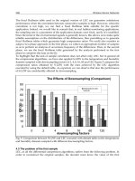
rapidly in the total region. The results further demonstrate that the hybrid sensor network
incorporating DFS with the O-LEACH protocol can evenly distribute the energy load among
nodes, therefore prolong the overall lifetime of the network.

6. Conclusion
We discussed several improved algorithms (protocols) that can be used for WSNs or hybrid
sensor networks with distributed fiber sensors involved. As sensor networks are much more
complicated in real applications, more thorough and careful optimization of routing
algorithms are required to meet specific requirements, such as real-time, long lifetime,
security, and so on.

7. References
[1] I. F. Akyildiz, W. Su, Y. Sankarasubramaniam, E. Cayirci (2002). A survey on sensor
networks, IEEE Communication Magazine, vol. 40, no.8, pp.102-114
[2] J. M. Kahn, R. H. Katz, and K. S. J. Pister (1999). Next century challenges: mobile
networking for smart dust, Proc. ACM MobiCom ’99, Washington DC, pp. 271–78
[3] V. Rodoplu and T. H. Meng (1999). Minimum energy mobile wireless networks, IEEE
JSAC, vol. 17, no. 8, pp.1333–1344
[4] K. Sohrabi et al. (2000). Protocols for self-organization of a wireless sensor network, IEEE
Pers. Commun., pp.16–27
[5] W. R. Heinzelman, A. Chandrakasan, and H. Balakrishnan (2000). Energy-efficient
communication protocol for wireless microsensor networks, IEEE Proc. Hawaii Int’l.
Conf. Sys. Sci., pp. 1–10
[6] X. Fan, Y. Song (2007). Improvement on LEACH protocol of wireless sensor network,
IEEE SENSORCOMM, pp.260-264
[7] H. Jeong, C S. Nam, Y S. Jeong, D R. Shin (2008). A mobile agent based LEACH in
wireless sensor network, Conf. on Advanced Comm. Technol. (ICACT), pp. 75-78
[8] Stephanie Lindsey and Cauligi S. Raghavendra (2002). PEGASIS: Power-Efficient
Gathering in Sensor Information System, 2002 IEEE Aerospace Conference, vol. 3,
pp.1125-1130

[9] X. Bao, D. J. Webb, and D. A. Jackson (1993). 32-km distributed temperature sensor using
Brillouin loss in optical fiber, Opt. Lett., vol. 18, pp.1561–1563.
[10] D. Garus, T. Gogolla, K. Krebber, F. Schliep (1997). Brillouin optical-fiber frequency-
domain analysis for distributed temperature and strain measurements, J. Lightwave
Technol., vol.15, no.4, pp.654-662
[11] S.M. Maughan, H. H. Kee, T. P. Newson (2001). A calibrated 27-km distributed fiber
temperature sensor based on microwave heterodyne detection of spontaneous
Brillouin scattered power, IEEE Photon. Technol. Lett., vol. 13, no 5, pp. 511-513
[12] J. C. Juarez, E. W. Maier, K. N. Choi, H. F. Taylor (2005). Distributed fiber-optic
intrusion sensor system, J. Lightwave Technol. vol.23, no.6, pp.2081-2087
[13] D. Iida, F. Ito (2008). Detection sensitivity of Brillouin scattering near Fresnel reflection
in BOTDR measurement, J. Lightwave Technol., vol. 26, no.4, pp.417-424
[14] D. Kedar and S. Arnon (2003). Laser ‘Firefly’ Clustering; a New Concept in
Atmospheric Probing, IEEE Photon. Tech. Lett., vol.15, no.1 pp. 1672–1624
s

[15] S. Teramoto, and T. Ohtsuki (2004). Optical wireless sensor network system using
corner cube retroreflectors (CCRs), IEEE Globecom’04, pp.1035-1039
[16] D. Kedar, S. Arnon (2005). Second generation laser firefly clusters: an improved
scheme for distributed sensing in the atmosphere, Appl. Opt., vol. 44, no.6, pp.984-
992
[17] Jamal N. AL-Karaki, Ahmed E. Kamal (2004). Routing Techniques in Wireless Sensor
Networks: A Survey, IEEE Wireless Communications, Dec.
[18] W. Heinzelman, J. Kulik, and H. Balakrishnan (1999). Adaptive Protocols for
Information Dissemination in Wireless Sensor Networks, Proc. 5th ACM/IEEE
Mobicom, Seattle, WA, pp. 174–85.
[19] J. Kulik, W. R. Heinzelman, and H. Balakrishnan (2002). Negotiation-Based Protocols
for Disseminating Information in Wireless Sensor Networks, Wireless Networks, vol.
8, pp. 169–85.
[20] Wendi Beth Heinzelman (2000). Application-Specific Protocol Architectures for

Wireless Networks (PhD), Boston: Massachusetts Institute of Technology
[21] Vivek Mhatre, Catherine Rosenberg (2004). Design guidelines for wireless sensor
networks: Communication, clustering and aggregation, Ad Hoc Networks, vol.2, no.1,
pp. 45-63
[22] Ning Xu, Sumit Rangwala, Krishna Kant Chintalapudi, Deepak Ganesan, Alan Broad,
Ramesh Govindan, Deborah Estrin (2004). A Wireless sensor network for structural
monitoring, Proc. 2nd international conference on Embedded networked sensor systems,
Baltimore, MD, USA, pp.13-24.
[23] Katayoun Sohrabi, Jay Gao, Vishal Ailawadhi , Gregory J.Pottie (2000). Protocols for
Self-organization of a Wireless Sensor Network, IEEE Personal Communications,
vol.7, no.5, pp.16-27
[24] ISO.16484-5, Building automation and control systems part 5 data communication
protocol, 2003.
[25] Stephanie Lindsey, Cauligi Raghavendra, Krishna M. Sivalingam (2002). Data
Gathering Algorithms in Sensor Networks Using Energy Metrics, IEEE Transactions
on Parallel and Distributed Systems, vol.13, no.9, pp.924-935



Hybrid Optical and Wireless Sensor Networks 319

Range-free Area Localization Scheme for Wireless Sensor Networks 321
Range-free Area Localization Scheme for Wireless Sensor Networks
Vijay R. Chandrasekhar, Winston K.G. Seah, Zhi Ang Eu and Arumugam P. Venkatesh
X

Range-free Area Localization Scheme
for Wireless Sensor Networks

Vijay R. Chandrasekhar

1
, Winston K.G. Seah
2
,
Zhi Ang Eu
3
and Arumugam P. Venkatesh
4

1
Stanford University, USA
*

2
Victoria University of Wellington, New Zealand
*

3
National University of Singapore
4
National University of Singapore

Abstract
For large wireless sensor networks, identifying the exact location of every sensor may not be
feasible and the cost may be very high. A coarse estimate of the sensors’ locations is usually
sufficient for many applications. In this chapter, we describe an efficient Area Localization
Scheme (ALS) for wireless sensor networks. ALS is a range-free scheme that tries to estimate
the position of every sensor within a certain area rather than its exact location. Furthermore,
the powerful sinks instead of the sensors handle all complex calculations. This reduces the
energy consumed by the sensors and helps extend the lifetime of the network. The

granularity of the areas estimated for each node can be easily adjusted by varying some
system parameters, thus making the scheme very flexible. We first study ALS under ideal
two-ray physical layer conditions (as a benchmark) before proceeding to test the scheme in
more realistic non-ideal conditions modelled by the two-ray physical layer model, Rayleigh
fading and lognormal shadowing. We compare the performance of ALS to range-free
localization schemes like APIT (Approximate Point In Triangle) and DV (Distance Vector)
Hop, and observe that the ALS outperforms them. We also implement ALS on an
experimental testbed and, show that at least 80% of nodes lie within a one-hop region of
their estimated areas. Both simulation and experimental results have verified that ALS is a
promising technique for range-free localization in large sensor networks.

Keywords: Localization, Wireless Sensor Network, Positioning, Range-free

1. Introduction
Deployment of low cost wireless sensors is envisioned to be a promising technique for
applications ranging from early warning systems for natural disasters (like tsunamis and


*
This work done by these authors in the Institute for Infocomm Research, Singapore.


17
Wireless Sensor Networks: Application-Centric Design322
wildfires), ecosystem monitoring, real-time health monitoring, and military surveillance.
The deployment and management of large scale wireless sensor networks is a challenge
because of the limited processing capability and power constraints on each sensor. Research
issues pertaining to wireless sensor networks, from the physical layer to the application
layer, as well as cross-layer issues like power management and topology management, have
been addressed[1]. Sensor network data is typically interpreted with reference to a sensor’s

location, e.g. reporting the occurrence of an event, tracking of a moving object or monitoring
the physical conditions of a region. Localization, the process of determining the location of a
sensor node in a wireless sensor network, is a challenging problem as reliance on technology
like GPS [2] is infeasible due to cost and energy constraints, and also physical constraints
like indoor environments.
In very large and dense wireless sensor networks, it may not be feasible to accurately
measure the exact location of every sensor and furthermore, a coarse estimate of the sensor’s
location may suffice for most applications. A preliminary design of the Area Localization
Scheme (ALS) [3] has been proposed, which can only function in an (unrealistic) ideal
channel and definitely not in a real environment with fading, shadowing and other forms of
interference. In this chapter, we describe algorithms and techniques that will enable the
Area Localization Scheme (ALS) to be deployable in a real environment. ALS is a centralized
range-free scheme that provides an estimation of a sensor’s location within a certain area,
rather than the exact coordinates of the sensor. The granularity of the location estimate is
determined by the size of areas which a sensor node falls within and this can be easily
adjusted by varying the system parameters. The advantage of this scheme lies in its
simplicity, as no measurements need to be made by the sensors. Since ALS is a range-free
scheme, we compare its performance to other range-free schemes like APIT (Approximate
Point In Triangle) [4], DV-Hop[5] and DHL (Density-aware Hopcount-based Localization)
[6]. To validate our schemes, we first use simulations developed in Qualnet[31] to evaluate
the performance of ALS and show that it outperforms other range-free localization schemes.
We then follow with an implementation of ALS on a wireless sensor network test bed and
conduct tests in both indoor and outdoor environments. We observe that at least 90% of
nodes lie within a 1-hop region of their estimated areas, i.e. within their individual
transmission radius.
The rest of the paper is organized as follows. Section 2 provides a survey of related work on
wireless sensor network localization. Section 3 then describes the key aspects of the basic
Area Localization Scheme. Section 4 describes the simulation environment and evaluates the
performance of the ALS and compares it to other range-free schemes. Section 5 discusses the
performance of the ALS evaluated on a wireless sensor network test bed for both indoor and

outdoor environments. This section also discusses how the ALS scheme is extended to a
generic physical layer model from the two-ray model used in the simulation studies. Section
6 presents our conclusions and plans for future work.



2. Related Work
A number of localization schemes have been proposed to date. The localization schemes
take into account a number of factors like the network topology, device capabilities, signal
propagation models and energy requirements. Most localization schemes require the
location of some nodes in the network to be known. Nodes whose locations are known are
referred to as anchor nodes or reference nodes in the literature. The localization schemes that
use reference nodes can be broadly classified into three categories: range-based schemes,
range-free schemes and schemes that use signal processing or probabilistic techniques
(hereafter referred to as probabilistic schemes). There also exist schemes that do not require
such reference locations in the network.

A. Range-based Schemes
In range-based schemes, the distance or angle measurements from a fixed set of reference
points are known. Multilateration, which encompass atomic, iterative and collaborative
multilateration techniques, are then used to estimate the location of each sensor node.
Range-based schemes use ToA (Time of Arrival), TDoA (Time Difference of Arrival), AOA
(Angle of Arrival) or RSSI (Received Signal Strength Indicator) to estimate their distances to
anchor nodes. UWB based localization schemes [7][8], GPS [2], Cricket [9] and other
schemes [11][12][13] use ToA or TDoA of acoustic or RF signals from multiple anchor nodes
for localization. However, the fast propagation of RF signals implies that a small error in
measurement could lead to large errors. Clock synchronization between multiple reference
nodes or between the sender and the receiver is also an extremely critical issue in schemes
that use ToA or TDoA. AOA allows sensor nodes to calculate the relative angles between
neighbouring nodes [14][15]. However, schemes that use AOA entail sensors and reference

nodes to be equipped with special antenna configurations which may not be feasible to
embed on each sensor. Complex non-linear equations also need to be solved[15]. Schemes
that use RSSI [16][17][18] have to deal with problems caused by large variances in reading,
multi-path fading, background interference and irregular signal propagation.

B. Range-free Schemes
Range-free localization schemes usually do not make use of any of the techniques
mentioned above to estimate distances to reference nodes, e.g. centroid scheme [19] and
APIT [4]. Range quantization methods like DV-Hop [5] and DHL [6] associate each 1-hop
connection with an estimated distance, while others apply RSSI quantization [20]. These
schemes also use multilateration techniques but rely on measures like hop count to estimate
distances to anchor nodes. Range-free schemes offer a less precise estimate of location
compared to range-based schemes.

C. Probabilistic Schemes
The third class of schemes use signal processing techniques or probabilistic schemes to do
localization. The fingerprinting scheme [21], which uses complex signal processing, is an
example of such a scheme. The major drawback of fingerprinting schemes is the substantial
effort required for generating a signal signature database, before localization can be
performed. Hence, it is not suitable for adhoc deployment scenarios in consideration.

D. Schemes without Anchor/Reference Points
The fourth class of schemes is different from the first three in that it does not require anchor
nodes or beacon signals. In [22], a central server models the network as a series of equations
representing proximity constraints between nodes, and then uses sophisticated optimization
Range-free Area Localization Scheme for Wireless Sensor Networks 323
wildfires), ecosystem monitoring, real-time health monitoring, and military surveillance.
The deployment and management of large scale wireless sensor networks is a challenge
because of the limited processing capability and power constraints on each sensor. Research
issues pertaining to wireless sensor networks, from the physical layer to the application

layer, as well as cross-layer issues like power management and topology management, have
been addressed[1]. Sensor network data is typically interpreted with reference to a sensor’s
location, e.g. reporting the occurrence of an event, tracking of a moving object or monitoring
the physical conditions of a region. Localization, the process of determining the location of a
sensor node in a wireless sensor network, is a challenging problem as reliance on technology
like GPS [2] is infeasible due to cost and energy constraints, and also physical constraints
like indoor environments.
In very large and dense wireless sensor networks, it may not be feasible to accurately
measure the exact location of every sensor and furthermore, a coarse estimate of the sensor’s
location may suffice for most applications. A preliminary design of the Area Localization
Scheme (ALS) [3] has been proposed, which can only function in an (unrealistic) ideal
channel and definitely not in a real environment with fading, shadowing and other forms of
interference. In this chapter, we describe algorithms and techniques that will enable the
Area Localization Scheme (ALS) to be deployable in a real environment. ALS is a centralized
range-free scheme that provides an estimation of a sensor’s location within a certain area,
rather than the exact coordinates of the sensor. The granularity of the location estimate is
determined by the size of areas which a sensor node falls within and this can be easily
adjusted by varying the system parameters. The advantage of this scheme lies in its
simplicity, as no measurements need to be made by the sensors. Since ALS is a range-free
scheme, we compare its performance to other range-free schemes like APIT (Approximate
Point In Triangle) [4], DV-Hop[5] and DHL (Density-aware Hopcount-based Localization)
[6]. To validate our schemes, we first use simulations developed in Qualnet[31] to evaluate
the performance of ALS and show that it outperforms other range-free localization schemes.
We then follow with an implementation of ALS on a wireless sensor network test bed and
conduct tests in both indoor and outdoor environments. We observe that at least 90% of
nodes lie within a 1-hop region of their estimated areas, i.e. within their individual
transmission radius.
The rest of the paper is organized as follows. Section 2 provides a survey of related work on
wireless sensor network localization. Section 3 then describes the key aspects of the basic
Area Localization Scheme. Section 4 describes the simulation environment and evaluates the

performance of the ALS and compares it to other range-free schemes. Section 5 discusses the
performance of the ALS evaluated on a wireless sensor network test bed for both indoor and
outdoor environments. This section also discusses how the ALS scheme is extended to a
generic physical layer model from the two-ray model used in the simulation studies. Section
6 presents our conclusions and plans for future work.



2. Related Work
A number of localization schemes have been proposed to date. The localization schemes
take into account a number of factors like the network topology, device capabilities, signal
propagation models and energy requirements. Most localization schemes require the
location of some nodes in the network to be known. Nodes whose locations are known are
referred to as anchor nodes or reference nodes in the literature. The localization schemes that
use reference nodes can be broadly classified into three categories: range-based schemes,
range-free schemes and schemes that use signal processing or probabilistic techniques
(hereafter referred to as probabilistic schemes). There also exist schemes that do not require
such reference locations in the network.

A. Range-based Schemes
In range-based schemes, the distance or angle measurements from a fixed set of reference
points are known. Multilateration, which encompass atomic, iterative and collaborative
multilateration techniques, are then used to estimate the location of each sensor node.
Range-based schemes use ToA (Time of Arrival), TDoA (Time Difference of Arrival), AOA
(Angle of Arrival) or RSSI (Received Signal Strength Indicator) to estimate their distances to
anchor nodes. UWB based localization schemes [7][8], GPS [2], Cricket [9] and other
schemes [11][12][13] use ToA or TDoA of acoustic or RF signals from multiple anchor nodes
for localization. However, the fast propagation of RF signals implies that a small error in
measurement could lead to large errors. Clock synchronization between multiple reference
nodes or between the sender and the receiver is also an extremely critical issue in schemes

that use ToA or TDoA. AOA allows sensor nodes to calculate the relative angles between
neighbouring nodes [14][15]. However, schemes that use AOA entail sensors and reference
nodes to be equipped with special antenna configurations which may not be feasible to
embed on each sensor. Complex non-linear equations also need to be solved[15]. Schemes
that use RSSI [16][17][18] have to deal with problems caused by large variances in reading,
multi-path fading, background interference and irregular signal propagation.

B. Range-free Schemes
Range-free localization schemes usually do not make use of any of the techniques
mentioned above to estimate distances to reference nodes, e.g. centroid scheme [19] and
APIT [4]. Range quantization methods like DV-Hop [5] and DHL [6] associate each 1-hop
connection with an estimated distance, while others apply RSSI quantization [20]. These
schemes also use multilateration techniques but rely on measures like hop count to estimate
distances to anchor nodes. Range-free schemes offer a less precise estimate of location
compared to range-based schemes.

C. Probabilistic Schemes
The third class of schemes use signal processing techniques or probabilistic schemes to do
localization. The fingerprinting scheme [21], which uses complex signal processing, is an
example of such a scheme. The major drawback of fingerprinting schemes is the substantial
effort required for generating a signal signature database, before localization can be
performed. Hence, it is not suitable for adhoc deployment scenarios in consideration.

D. Schemes without Anchor/Reference Points
The fourth class of schemes is different from the first three in that it does not require anchor
nodes or beacon signals. In [22], a central server models the network as a series of equations
representing proximity constraints between nodes, and then uses sophisticated optimization
Wireless Sensor Networks: Application-Centric Design324
techniques to estimate the location of every node in the network. In [23], Capkun et al.
propose an infrastructure-less GPS-free positioning algorithm.

E. Area-based Localization
Most of the localization schemes mentioned above calculate a sensor node’s exact position,
except for [4], which uses an area-based approach. In [4], anchor nodes send out beacon
packets at the highest power level that they can. A theoretical method, based on RSSI
measurements, called Approximate Point in Triangle (APIT), is defined to determine
whether a point lies inside a triangle formed by connecting three anchor nodes. A sensor
node uses the APIT test with different combinations of three audible anchor nodes (audible
anchors are anchor nodes from which beacon packets are received) until all combinations
are exhausted. Each APIT test determines whether or not the node lies inside a distinct
triangular region. The intersection of all the triangular regions is then considered to estimate
the area in which the sensor is located. The APIT algorithm performs well when the average
number of audible anchors is high (for example, more than 20). As a result, a major
drawback of the algorithm is that it is highly computationally intensive. An average of 20
audible anchors would imply that the intersection of
20
C
3
= 1140 areas need to be considered.
Furthermore, the algorithm performs well only when the anchor nodes are randomly
distributed throughout the network, which is not always feasible in a real deployment
scenario.

3. Area Localization Scheme Fundamentals
In ALS, the nodes in the wireless sensor network are divided into three categories according
to their different functions: reference nodes, sensor nodes and sinks.

A. Reference/Anchor nodes
The main responsibility of the reference/anchor (both terms will be used interchangeably)
nodes is to send out beacon signals to help sensor nodes locate themselves. Reference nodes

are either equipped with GPS to provide accurate location information or placed in pre-
determined locations. In addition, the reference nodes can send out radio signals at varying
power levels as required. For an Ideal Isotropic Antenna, the received power at a distance d
from the transmitter is given by:

2
4







d
GGPP
rttr



(1)

while the two-ray ground reflection model considers both the direct path and a ground
reflection path, and the received power at a distance d is given by:

4
22
d
PGGhh
P

ttrtr
r

for


rt
hh
d
4

(2)

where P
r
is the received power, P
t
is the transmitted power, d is the distance between the
transmitter and receiver,

is the wavelength and, h
t
and h
r
are the heights of the transmitter
and receiver respectively. G
t
and G
r
represent the gains of the transmitter and receiver

respectively in equations (1) and (2).
From the above equations, it can be clearly seen that if the received power is fixed at a
certain value, the radio signal with a higher transmitted power reaches a greater distance.
Using one of the physical layer models described above and the threshold power that each
sensor can receive, the reference node can calculate the power required to reach different
distances. Each reference node then devises a set of increasing power levels such that the
highest power level can cover the entire area in consideration. The reference nodes then
broadcast several rounds of radio signals. The beacon packet contains the ID of the reference
node and the power level at which the signal is transmitted (which can be simply
represented by an integer value, as explained below.)
Let PS denote the set of increasing power levels of beacon signals sent out by a reference
node. For now, let us assume that all the reference nodes in the system send out the same set
PS of beacon signals. In the ALS scheme, a sensor node simply listens and records the power
levels of beacon signals it receives from each reference node. In real environments, small
scale fading and shadowing can cause the power levels received by the sensor nodes to vary
significantly from the expected power levels calculated by the path loss models in equations
(1) and (2). Sending out beacon signals in the set PS only once might lead to inaccurate
beacon reception by sensor nodes. As a result, the reference nodes send out the beacon
signals in set PS multiple times. The sensor nodes can then calculate the statistical average
(mode or mean) of the received power levels from each reference node.
Let the number of power levels in set PS be denoted by N
p
and the N
p
power levels in set PS
be represented by P
1
,P
2
, P

3
,…,P
Np
. The power levels P
1
, P
2
, P
3
,…,P
Np
can be represented by
simple integers, e.g. increasing values corresponding to increasing power levels; therefore
sensor nodes only need to take note of these integer values that are contained in the beacon
packets and the hardware design can be kept simple as there is no need for accurate
measurement of the received power level. Let the number of times that the same set of
beacon signals PS are sent out be denoted by N
r
, also referred to as the number of rounds.
The power MP in dB required to cover the entire area is calculated from equation (1) or (2),
based on the physical layer model in consideration. The power LP in dB required to cover a
small distance

(say 10 m) is also calculated. The values P
1
,P
2
, P
3
,…,P

Np
are then set to be
N
p
uniformly distributed values in the range [LP, MP] in the dB scale. The simple procedure
followed by the reference nodes is shown below:

1 for i = 1: Nr
2 for j=1: N
p

3 Send beacon signal at power levelP
j

4 end for
5 end for

The transmissions by the different reference nodes do not need to be synchronized.
However, the reference nodes schedule the beacon signal transmissions so to avoid
collisions. The transmitted set of power levels PS need not be the same for all the reference
nodes, and can be configured by the network administrator. Also, the set of power levels PS
need not be uniformly distributed too. It is also not necessary for the reference nodes to
Range-free Area Localization Scheme for Wireless Sensor Networks 325
techniques to estimate the location of every node in the network. In [23], Capkun et al.
propose an infrastructure-less GPS-free positioning algorithm.

E. Area-based Localization
Most of the localization schemes mentioned above calculate a sensor node’s exact position,
except for [4], which uses an area-based approach. In [4], anchor nodes send out beacon
packets at the highest power level that they can. A theoretical method, based on RSSI

measurements, called Approximate Point in Triangle (APIT), is defined to determine
whether a point lies inside a triangle formed by connecting three anchor nodes. A sensor
node uses the APIT test with different combinations of three audible anchor nodes (audible
anchors are anchor nodes from which beacon packets are received) until all combinations
are exhausted. Each APIT test determines whether or not the node lies inside a distinct
triangular region. The intersection of all the triangular regions is then considered to estimate
the area in which the sensor is located. The APIT algorithm performs well when the average
number of audible anchors is high (for example, more than 20). As a result, a major
drawback of the algorithm is that it is highly computationally intensive. An average of 20
audible anchors would imply that the intersection of
20
C
3
= 1140 areas need to be considered.
Furthermore, the algorithm performs well only when the anchor nodes are randomly
distributed throughout the network, which is not always feasible in a real deployment
scenario.

3. Area Localization Scheme Fundamentals
In ALS, the nodes in the wireless sensor network are divided into three categories according
to their different functions: reference nodes, sensor nodes and sinks.

A. Reference/Anchor nodes
The main responsibility of the reference/anchor (both terms will be used interchangeably)
nodes is to send out beacon signals to help sensor nodes locate themselves. Reference nodes
are either equipped with GPS to provide accurate location information or placed in pre-
determined locations. In addition, the reference nodes can send out radio signals at varying
power levels as required. For an Ideal Isotropic Antenna, the received power at a distance d
from the transmitter is given by:

2
4







d
GGPP
rttr



(1)

while the two-ray ground reflection model considers both the direct path and a ground
reflection path, and the received power at a distance d is given by:

4
22
d
PGGhh
P
ttrtr
r

for



rt
hh
d
4

(2)

where P
r
is the received power, P
t
is the transmitted power, d is the distance between the
transmitter and receiver,

is the wavelength and, h
t
and h
r
are the heights of the transmitter
and receiver respectively. G
t
and G
r
represent the gains of the transmitter and receiver
respectively in equations (1) and (2).
From the above equations, it can be clearly seen that if the received power is fixed at a
certain value, the radio signal with a higher transmitted power reaches a greater distance.
Using one of the physical layer models described above and the threshold power that each
sensor can receive, the reference node can calculate the power required to reach different

distances. Each reference node then devises a set of increasing power levels such that the
highest power level can cover the entire area in consideration. The reference nodes then
broadcast several rounds of radio signals. The beacon packet contains the ID of the reference
node and the power level at which the signal is transmitted (which can be simply
represented by an integer value, as explained below.)
Let PS denote the set of increasing power levels of beacon signals sent out by a reference
node. For now, let us assume that all the reference nodes in the system send out the same set
PS of beacon signals. In the ALS scheme, a sensor node simply listens and records the power
levels of beacon signals it receives from each reference node. In real environments, small
scale fading and shadowing can cause the power levels received by the sensor nodes to vary
significantly from the expected power levels calculated by the path loss models in equations
(1) and (2). Sending out beacon signals in the set PS only once might lead to inaccurate
beacon reception by sensor nodes. As a result, the reference nodes send out the beacon
signals in set PS multiple times. The sensor nodes can then calculate the statistical average
(mode or mean) of the received power levels from each reference node.
Let the number of power levels in set PS be denoted by N
p
and the N
p
power levels in set PS
be represented by P
1
,P
2
, P
3
,…,P
Np
. The power levels P
1

, P
2
, P
3
,…,P
Np
can be represented by
simple integers, e.g. increasing values corresponding to increasing power levels; therefore
sensor nodes only need to take note of these integer values that are contained in the beacon
packets and the hardware design can be kept simple as there is no need for accurate
measurement of the received power level. Let the number of times that the same set of
beacon signals PS are sent out be denoted by N
r
, also referred to as the number of rounds.
The power MP in dB required to cover the entire area is calculated from equation (1) or (2),
based on the physical layer model in consideration. The power LP in dB required to cover a
small distance

(say 10 m) is also calculated. The values P
1
,P
2
, P
3
,…,P
Np
are then set to be
N
p
uniformly distributed values in the range [LP, MP] in the dB scale. The simple procedure

followed by the reference nodes is shown below:

1 for i = 1: Nr
2 for j=1: N
p

3 Send beacon signal at power levelP
j

4 end for
5 end for

The transmissions by the different reference nodes do not need to be synchronized.
However, the reference nodes schedule the beacon signal transmissions so to avoid
collisions. The transmitted set of power levels PS need not be the same for all the reference
nodes, and can be configured by the network administrator. Also, the set of power levels PS
need not be uniformly distributed too. It is also not necessary for the reference nodes to
Wireless Sensor Networks: Application-Centric Design326
know each other’s position and levels of transmitted power, but there should be at least one
sink or a central agent that stores the location information of all the reference nodes.

B. Sensor node
A sensor node is a unit device that monitors the environment. Sensors typically have limited
computing capability, storage capacity, communications range and battery power. Due to
power constraints, it is not desirable forsensor nodes to make complex calculations and send
out information frequently.

1) Signal Coordinate Representation:
In the ALS scheme, the sensors save a list of reference nodes and their respective transmitted
power levels and forward the information to the nearest sink when requested or appended

to sensed data. The sinks use this information to identify the area in which the sensors
reside in. However, if the number of reference nodes is large, the packets containing location
information may be long, which might result in more traffic in the network. A naming
scheme is hence designed.
The sensor nodes use a signal coordinate representation to indicate their location
information to the sinks. Power contour lines can be drawn on an area based on the set of
beacon signal power levels PS transmitted by each reference node, and their corresponding
distances travelled. The power contour lines divide the region in consideration into many
sub-regions (which we refer to as areas) as shown in Figure 1 below. Each area in the region
can be represented by a unique set of n coordinates, hereafter referred to as the signal
coordinate.
Suppose there are n reference nodes, which are referred to as R
1
, R
2,… ,
and R
n.
For a sensor in
an area, let the lowest transmitted power levels it receives from the n reference nodes be S
1
,
S
2, …,
and S
n
respectively. S
1
, S
2, …,
and S

n
are simple integer numbers indicating the different
power levels rather than the actual signal strengths. The mappings between integer levels
and the actual power values are saved at the reference nodes and sinks. The signal
coordinate is defined as the representation < S
1
, S
2, …,
S
n
> such that each S
i
, the i
th
element, is
the lowest power level received from R
i
.
For example, consider a square region with reference nodes at the four corners, as shown in
Figure 1. In this case, the set of power levels PS is the same for all the four reference nodes
and there are three power levels in the set PS. The smallest power level in the power set PS
is represented by the integer 1 while the highest power level is represented by the integer 3.
For each node, the contour lines drawn on the region represent the farthest distances that
the beacon signals at each power level can travel. Contour lines for beacon power levels 1
and 2 are drawn. The power level 3 for each corner reference node can reach beyond the
corner that is diagonally opposite to it and so, its corresponding contour line is not seen on
the square region. Thus, for each reference node, the two contour lines corresponding to
power levels 1 and 2 divide the region into three (arc) areas.
Fi
g

Fo
fr
o
si
g
th
e
re
p
sq
u
st
a
n
o
co
o
T
h
tr
a
<
S
ne
co
o
th
e

2)
In

re
c
g
. 1. Example of
A
r a sensor node
i
o
m reference no
d
g
nals at power le
v
e
sensor from r
e
p
resented b
y
th
e
u
are region can
b
a
ted in the si
g

na
o
de i forms the
o
rdinate to ident
i
h
us, if all the sen
s
a
nsmitted b
y
ea
S
1
,S
2
,…,S
n
> to in
d
ed to
g
et infor
m
o
rdinate in its re
q
e
ir ow

n
to see if
t
Algorithm

the ALS schem
e
c
ords the inform
A
LS under ideal
i
i
n the shaded ar
e
d
es 1, 2 and 3 is

v
els 2 and 3 fro
m
e
ference node 4
i
e
unique si
g
nal
c
b

e represented b
y
l coordinate def
i
i
th
element of
t
i
f
y
the area in w
h
s
ors and sinks a
g
ch reference n
o
d
icate their area
l
m
atio
n
from se
n
q
uest and the se
n
t

he
y
lie in the rel
e
e
, the sensor nod
ation that it rec
e
i
sotropic conditi
o
e
a(lower ri
g
ht) i
n

3.The sensor n
o
m
reference node
4
i
s 2. As a result
,
c
oordinate <3,3,
3
y
a unique si

g
na
l
i
nition, the lowe
t
he si
g
nal coor
d
h
ich the
y
are loca
g
ree in advance
o
o
de, the sensor
l
ocation informa
t
n
sors specific to

n
sors simpl
y
co
m

e
vant area.
e simpl
y
listens
e
ives from them.

o
ns; shaded re
g
io
n
n
Fig. 1, the lowe
s
o
de in the shade
d
4
. So, the lowest
p
,
the shaded ar
e
3
,2>. Similarl
y
,
e

l
coordinate, as
s
st power level r
e
d
inate. Sensors
u
ted.
on
the set(s) of
b
nodes can use
t
io
n
to the sinks.


a certain area,
m
pare the incomi
to si
g
nals from
a

A sensor node
a

n is <3, 3, 3, 2>
s
t power level r
e
d
area receives
b
p
ower level recei
v
e
a in the fi
g
ure
c
e
very other area
s
how
n
in the fi
gu
e
ceived from re
f
u
se this unique
b
eacon power le
v

the si
g
nal coo
r

Similarly, when

it includes the
n
g
signal coordi
n
a
ll reference nod
e
a
t a particular l
o
e
ceived
b
eacon
v
ed by
c
an be
in the
u
re. As
f

erence
si
g
nal
v
els PS
r
dinate

a sink
signal
n
ate to
e
s and
o
cation
Range-free Area Localization Scheme for Wireless Sensor Networks 327
know each other’s position and levels of transmitted power, but there should be at least one
sink or a central agent that stores the location information of all the reference nodes.

B. Sensor node
A sensor node is a unit device that monitors the environment. Sensors typically have limited
computing capability, storage capacity, communications range and battery power. Due to
power constraints, it is not desirable forsensor nodes to make complex calculations and send
out information frequently.

1) Signal Coordinate Representation:
In the ALS scheme, the sensors save a list of reference nodes and their respective transmitted
power levels and forward the information to the nearest sink when requested or appended

to sensed data. The sinks use this information to identify the area in which the sensors
reside in. However, if the number of reference nodes is large, the packets containing location
information may be long, which might result in more traffic in the network. A naming
scheme is hence designed.
The sensor nodes use a signal coordinate representation to indicate their location
information to the sinks. Power contour lines can be drawn on an area based on the set of
beacon signal power levels PS transmitted by each reference node, and their corresponding
distances travelled. The power contour lines divide the region in consideration into many
sub-regions (which we refer to as areas) as shown in Figure 1 below. Each area in the region
can be represented by a unique set of n coordinates, hereafter referred to as the signal
coordinate.
Suppose there are n reference nodes, which are referred to as R
1
, R
2,… ,
and R
n.
For a sensor in
an area, let the lowest transmitted power levels it receives from the n reference nodes be S
1
,
S
2, …,
and S
n
respectively. S
1
, S
2, …,
and S

n
are simple integer numbers indicating the different
power levels rather than the actual signal strengths. The mappings between integer levels
and the actual power values are saved at the reference nodes and sinks. The signal
coordinate is defined as the representation < S
1
, S
2, …,
S
n
> such that each S
i
, the i
th
element, is
the lowest power level received from R
i
.
For example, consider a square region with reference nodes at the four corners, as shown in
Figure 1. In this case, the set of power levels PS is the same for all the four reference nodes
and there are three power levels in the set PS. The smallest power level in the power set PS
is represented by the integer 1 while the highest power level is represented by the integer 3.
For each node, the contour lines drawn on the region represent the farthest distances that
the beacon signals at each power level can travel. Contour lines for beacon power levels 1
and 2 are drawn. The power level 3 for each corner reference node can reach beyond the
corner that is diagonally opposite to it and so, its corresponding contour line is not seen on
the square region. Thus, for each reference node, the two contour lines corresponding to
power levels 1 and 2 divide the region into three (arc) areas.
Fi
g

Fo
fr
o
si
g
th
e
re
p
sq
u
st
a
n
o
co
o
T
h
tr
a
<
S
ne
co
o
th
e

2)
In

re
c
g
. 1. Example of
A
r a sensor node
i
o
m reference no
d
g
nals at power le
v
e
sensor from r
e
p
resented b
y
th
e
u
are region can
b
a
ted in the si
g

na
o
de i forms the
o
rdinate to ident
i
h
us, if all the sen
s
a
nsmitted b
y
ea
S
1
,S
2
,…,S
n
> to in
d
ed to
g
et infor
m
o
rdinate in its re
q
e
ir ow

n
to see if
t
Algorithm

the ALS schem
e
c
ords the inform
A
LS under ideal
i
i
n the shaded ar
e
d
es 1, 2 and 3 is

v
els 2 and 3 fro
m
e
ference node 4
i
e
unique si
g
nal
c
b

e represented b
y
l coordinate def
i
i
th
element of
t
i
fy the area in w
h
s
ors and sinks a
g
ch reference n
o
d
icate their area
l
m
atio
n
from se
n
q
uest and the se
n
t
he
y

lie in the rel
e
e
, the sensor nod
ation that it rec
e
i
sotropic conditi
o
e
a(lower ri
g
ht) i
n

3.The sensor n
o
m
reference node
4
i
s 2. As a result
,
c
oordinate <3,3,
3
y
a unique si
g
na

l
i
nition, the lowe
t
he si
g
nal coor
d
h
ich they are loca
g
ree in advance
o
o
de, the sensor
l
ocation informa
t
n
sors specific to

n
sors simply co
m
e
vant area.
e simpl
y
listens
e

ives from them.

o
ns; shaded re
g
io
n
n
Fig. 1, the lowe
s
o
de in the shade
d
4
. So, the lowest
p
,
the shaded ar
e
3
,2>. Similarl
y
,
e
l
coordinate, as
s
st power level r
e
d

inate. Sensors
u
ted.
on
the set(s) of
b
nodes can use
t
io
n
to the sinks.


a certain area,
m
pare the incomi
to si
g
nals from
a

A sensor node
a

n is <3, 3, 3, 2>
s
t power level r
e
d
area receives

b
p
ower level recei
v
e
a in the fi
g
ure
c
e
very other area
s
how
n
in the fi
gu
e
ceived from re
f
u
se this unique
b
eacon power le
v
the si
g
nal coo
r

Similarly, when

it includes the
ng signal coordi
n
a
ll reference nod
e
a
t a particular l
o
e
ceived
b
eacon
v
ed by
c
an be
in the
u
re. As
f
erence
si
g
nal
v
els PS
r
dinate

a sink
signal
n
ate to
e
s and
o
cation
Wireless Sensor Networks: Application-Centric Design328
may receive localization signals (beacon messages)at different power levels from the same
reference node, as explained above. The sensor records its signal coordinate and forwards
the information to the sink(s) using the existing data delivery scheme, as and when
requested.
Let the signal coordinate of a node be denoted <S
1
, S
2
,…,S
n
> where n is the number of
reference nodes. A sensor node uses variables L
11
, L
12,
…,L
1Nr
to represent the lowest power
levels received by the sensor from reference node 1 during rounds 1 to N
r.

Similarly, let
L
i1
, L
i2
,…,L
iNr
represent the lowest power levels received by the sensor from reference node i
during rounds 1 to N
r.
Let the number of reference nodes be n. Initially, all the values
L
11
, L
12,
…, L
1Nr
, L
21
, L
22
, …, L
2Nr
, …, L
n1
, L
n2
, …, L
nNr
are set to zero. The zeros imply that the

sensor nodes have received no signals from the reference nodes.
The pseudo-code running on each sensor node is shown below. After initialization, the
sensor nodes start an infinite loop to receive beacon messages from reference nodes and
follow the algorithm shown below. Since a reference node sends out several rounds of
beacon signals, the sensor node may hear multiple rounds of beacon signals from the same
reference node. If the sensor receives a signal from reference node i for the first time during
round j, it sets L
ij
to be the lowest received power level for that round; otherwise, if the
received power level from reference node i in round j is lower than the current value in
L
ij
, L
ij
is set to the latest received power level. After all the reference nodes have completed
sending out beacon messages, the power levels L
i1
to L
iNr
on each sensor represent the lowest
power levels received from reference node i during rounds 1 to N
r
respectively.

Initialization:
1 for i=1 to n
2 for j = 1 to Nr
3 L
ij
= 0

4 end for
5 end for
Loop:
1 Receive a message
2 if (the message is from reference nodei during round j)
3 if (L
ij
= 0 || received power level <L
ij
) ; received power level  integer
representation
4 L
ij
= received power level
5 end if
6 end if

Each reference node sends out beacon signals at all the power levels in the set PS N
r
times
(N
r
rounds). In real conditions, fading and shadowing can cause the power levels to vary
erratically about the expected signal strength predicted by the large scale fading model.
Hence, the lowest signal power level received by a sensor from a reference node need not be
the same for all the rounds 1 to N
r
, i.e. all the values L
i1
to L

iNr
need not be the same. One is
then faced with the problem of deciding which value L
ix
to pick as S
i,
the i
th
element of the
signal coordinate.
Hence, a threshold value CONFIDENCE_LEVEL is defined. This parameter represents the
confidence level with which the values S
1
, S
2
, …, S
n
can be estimated, and is an operational
va
to
fr
e
i
th
fr
e
{L
i
fu
r

Fi
g
lue that end use
r
80% of N
r
in o
u
e
quenc
y

g
reater
t
element in the
n
e
quenc
y

g
reater
t
1
L
iNr
} are consi
d

r
ther refinement
m
g
. 2. Illustration
o
r
s can specif
y
to
u
r performance
t
han CONFIDEN
C
n
ode’s si
g
nal c
o
t
ha
n
CONFIDE
N
d
ered possible c
a
m
a

y
be necessar
y
(a) Bl
a
(Black

(b) Bla
c
o
f Si
g
nal Coordin
suit their requir
e
studies. If there
C
E_LEVEL in th
e
o
ordinate, i.e. S
i
N
CE_LEVEL, the
n
a
ndidates of the
i
y
.

a
ck re
g
ion <{2,3
}

Red) regions <
{
c
k re
g
ion <{2,3}
,
ate Representati
o
e
ments. For exa
m
is a power lev
e
e
set {L
i
, …, L
iNr
},

= L
ix
. If there i

s
n
all the distinct
p
i
th
element of the

}
, 3, 3, 3>.
1,2,3}, 3,3,3>
,
3, 3,{2,3}>
on

m
ple, this value
w
e
l L
ix
that occur

then L
ix
is set to

s
no power lev
e

p
ower levels in
t

signal coordina
t


w
as set
s with

be the
e
l with
t
he set
t
e, and
Range-free Area Localization Scheme for Wireless Sensor Networks 329
may receive localization signals (beacon messages)at different power levels from the same
reference node, as explained above. The sensor records its signal coordinate and forwards
the information to the sink(s) using the existing data delivery scheme, as and when
requested.
Let the signal coordinate of a node be denoted <S
1
, S
2
,…,S
n

> where n is the number of
reference nodes. A sensor node uses variables L
11
, L
12,
…,L
1Nr
to represent the lowest power
levels received by the sensor from reference node 1 during rounds 1 to N
r.
Similarly, let
L
i1
, L
i2
,…,L
iNr
represent the lowest power levels received by the sensor from reference node i
during rounds 1 to N
r.
Let the number of reference nodes be n. Initially, all the values
L
11
, L
12,
…, L
1Nr
, L
21
, L

22
, …, L
2Nr
, …, L
n1
, L
n2
, …, L
nNr
are set to zero. The zeros imply that the
sensor nodes have received no signals from the reference nodes.
The pseudo-code running on each sensor node is shown below. After initialization, the
sensor nodes start an infinite loop to receive beacon messages from reference nodes and
follow the algorithm shown below. Since a reference node sends out several rounds of
beacon signals, the sensor node may hear multiple rounds of beacon signals from the same
reference node. If the sensor receives a signal from reference node i for the first time during
round j, it sets L
ij
to be the lowest received power level for that round; otherwise, if the
received power level from reference node i in round j is lower than the current value in
L
ij
, L
ij
is set to the latest received power level. After all the reference nodes have completed
sending out beacon messages, the power levels L
i1
to L
iNr
on each sensor represent the lowest

power levels received from reference node i during rounds 1 to N
r
respectively.

Initialization:
1 for i=1 to n
2 for j = 1 to Nr
3 L
ij
= 0
4 end for
5 end for
Loop:
1 Receive a message
2 if (the message is from reference nodei during round j)
3 if (L
ij
= 0 || received power level <L
ij
) ; received power level  integer
representation
4 L
ij
= received power level
5 end if
6 end if

Each reference node sends out beacon signals at all the power levels in the set PS N
r
times

(N
r
rounds). In real conditions, fading and shadowing can cause the power levels to vary
erratically about the expected signal strength predicted by the large scale fading model.
Hence, the lowest signal power level received by a sensor from a reference node need not be
the same for all the rounds 1 to N
r
, i.e. all the values L
i1
to L
iNr
need not be the same. One is
then faced with the problem of deciding which value L
ix
to pick as S
i,
the i
th
element of the
signal coordinate.
Hence, a threshold value CONFIDENCE_LEVEL is defined. This parameter represents the
confidence level with which the values S
1
, S
2
, …, S
n
can be estimated, and is an operational
va
to

fr
e
i
th
fr
e
{L
i
fu
r

Fi
g
lue that end use
r
80% of N
r
in o
u
e
quenc
y

g
reater
t
element in the
n
e
quenc

y

g
reater
t
1
L
iNr
} are consi
d
r
ther refinement
m
g
. 2. Illustration
o
r
s can specif
y
to
u
r performance
t
han CONFIDEN
C
n
ode’s si
g
nal c
o

t
ha
n
CONFIDE
N
d
ered possible c
a
m
a
y
be necessar
y
(a) Bl
a
(Black

(b) Bla
c
o
f Si
g
nal Coordin
suit their requir
e
studies. If there
C
E_LEVEL in th
e
o

ordinate, i.e. S
i
N
CE_LEVEL, the
n
a
ndidates of the
i
y
.
a
ck re
g
ion <{2,3
}

Red) regions <
{
ck region <{2,3}
,
ate Representati
o
e
ments. For exa
m
is a power lev
e
e
set {L
i

, …, L
iNr
},

= L
ix
. If there i
s
n
all the distinct
p
i
th
element of the

}
, 3, 3, 3>.
1,2,3}, 3,3,3>
,
3, 3,{2,3}>
on

m
ple, this value
w
e
l L
ix
that occur

then L
ix
is set to

s
no power lev
e
p
ower levels in
t

signal coordina
t


w
as set
s with

be the
e
l with
t
he set
t
e, and
Wireless Sensor Networks: Application-Centric Design330
This concept is further illustrated by a couple of examples and we assume the same scenario
as in Fig. 1. In Fig. 1, we have assumed ideal isotropic channel conditions and each element
in the signal coordinate has been ascertained with a high confidence level.

Fig. 2 illustrates scenarios of non-ideal channel conditions where beacons messages may be lost.
Fig. 2(a) shows the case <{2,3},3,3,3>, where the first element of the signal coordinate is either
1 or 2. This happens when the lowest power level received from reference 1 during the N
r

rounds of beacon messages oscillates between 1 and 2. Both values (1 and 2) can be
considered as possible candidates for S
1,
if no power level L
1x
occurs with frequency greater
than CONFIDENCE_LEVEL in the set {L
11
, , L
1Nr
}. The union of the black and red regions in
Fig. 2(a) represents the region <0, 3, 3, 3>, where the value of 0 implies that there is no
information available on the first element. This could happen in the case when no beacon
packets are received from reference node 1, and the signal coordinate region <{1,2,3},3,3,3>
is considered as a result. Thus, every element S
i
in the set <S
1
, S
2
, …,S
n
> need not be a
unique value, but could be a set of values as shown in Fig. 2(b). While more than one

element of a signal coordinate may have multiple values, we consider a signal coordinate to
be valid only if at least half of its values have been determined with a high confidence level.
From the above description, it can be clearly seen that the sensor nodes do not perform any
complicated calculations to estimate their location. Neither do they need to exchange
information with their neighbours.

C. Sink
In wireless sensor networks, data from sensor nodes are forwarded to a sink for processing.
From a hardware point of view, a sink usually has much higher computing and data
processing capabilities than a sensor node. In ALS, a sensor node sends its signal coordinate
(location information) to a sink according to the data delivery scheme in use. The sensor
itself does not know the exact location of the area in which it resides nor does it know what
its signal coordinate represents. It is up to the sink(s) to determine the sensor’s location
based on the signal coordinate information obtained from the sensor. One assumption of the
ALS scheme is that the sink knows the positions of all the reference nodes and their
respective transmitted power levels, whether by directly communicating with the reference
nodes, or from a central server, which contains this information. Therefore, with the
knowledge of the physical layer model and signal propagation algorithms, the sink is able to
derive the map of areas based on the information of the transmitted signals from the
reference nodes. With the map and the signal coordinate information, the sink can then
determine which area a sensor is in from the received data, tagged with the signal
coordinate.
In the ALS scheme, the choosing of the signal propagation model plays an important part in
the estimation accuracy. For different networks, different signal propagation models can be
used to draw out the signal map according to the physical layer conditions. An irregular signal
model could divide the whole region into many differently shaped areas, as shown in Fig. 3.
Any adjustments made to the underlying physical layer model will have no impact on the
sensor nodes, which just need to measure their signal coordinates and forward them to the
sink. An immediate observation is the diverse area granularity, which affects the accuracy of
the location estimation. The granularity issue will be discussed in the next section.

A key advantage of ALS is its simplicity for the sensors with all the complex calculations
done by the sink. Thus, the localization process consumes little power at the sensor nodes,
helps to extend the life of the whole network. Furthermore, it has a covert feature whereby
anyone eavesdropping on the transmission will not be able to infer the location of sensors
from the signal coordinates contained in the packets.


Fig. 3. Irregular contour lines arising from a non-ideal signal model

4. Performance Evaluation of ALS
We evaluate ALS using simulations as well as field experimentation using commercially
available wireless sensor nodes.

A. Performance metrics for ALS
The metrics, accuracy and granularity, are used to evaluate the performance of the scheme.
High levels of accuracy and granularity are desired; however, accuracy begins to suffer as
granularity increases, since the probability of estimating the location of a node correctly in a
smaller area decreases. Hence, in order to have a fair evaluation of ALS, we normalize the
accuracy with respect to the granularity or average area estimate, that is, normalized accuracy
= accuracy / average area estimate.
Another metric, average error, is defined to compare the performance of ALS to other range
free schemes. The Center of Gravity (COG) or centroid of the final area estimate is assumed
to be location of the node. Average error is then defined to be the average of the Euclidian
distances between the original and estimated locations for all the nodes in the network.

B. Simulation scenario and parameters
The QUALNET 3.8 simulation environment is used to evaluate the performance of ALS. The
system parameters used in our simulations are described below.
Range-free Area Localization Scheme for Wireless Sensor Networks 331
This concept is further illustrated by a couple of examples and we assume the same scenario

as in Fig. 1. In Fig. 1, we have assumed ideal isotropic channel conditions and each element
in the signal coordinate has been ascertained with a high confidence level.

Fig. 2 illustrates scenarios of non-ideal channel conditions where beacons messages may be lost.
Fig. 2(a) shows the case <{2,3},3,3,3>, where the first element of the signal coordinate is either
1 or 2. This happens when the lowest power level received from reference 1 during the N
r

rounds of beacon messages oscillates between 1 and 2. Both values (1 and 2) can be
considered as possible candidates for S
1,
if no power level L
1x
occurs with frequency greater
than CONFIDENCE_LEVEL in the set {L
11
, , L
1Nr
}. The union of the black and red regions in
Fig. 2(a) represents the region <0, 3, 3, 3>, where the value of 0 implies that there is no
information available on the first element. This could happen in the case when no beacon
packets are received from reference node 1, and the signal coordinate region <{1,2,3},3,3,3>
is considered as a result. Thus, every element S
i
in the set <S
1
, S
2
, …,S
n

> need not be a
unique value, but could be a set of values as shown in Fig. 2(b). While more than one
element of a signal coordinate may have multiple values, we consider a signal coordinate to
be valid only if at least half of its values have been determined with a high confidence level.
From the above description, it can be clearly seen that the sensor nodes do not perform any
complicated calculations to estimate their location. Neither do they need to exchange
information with their neighbours.

C. Sink
In wireless sensor networks, data from sensor nodes are forwarded to a sink for processing.
From a hardware point of view, a sink usually has much higher computing and data
processing capabilities than a sensor node. In ALS, a sensor node sends its signal coordinate
(location information) to a sink according to the data delivery scheme in use. The sensor
itself does not know the exact location of the area in which it resides nor does it know what
its signal coordinate represents. It is up to the sink(s) to determine the sensor’s location
based on the signal coordinate information obtained from the sensor. One assumption of the
ALS scheme is that the sink knows the positions of all the reference nodes and their
respective transmitted power levels, whether by directly communicating with the reference
nodes, or from a central server, which contains this information. Therefore, with the
knowledge of the physical layer model and signal propagation algorithms, the sink is able to
derive the map of areas based on the information of the transmitted signals from the
reference nodes. With the map and the signal coordinate information, the sink can then
determine which area a sensor is in from the received data, tagged with the signal
coordinate.
In the ALS scheme, the choosing of the signal propagation model plays an important part in
the estimation accuracy. For different networks, different signal propagation models can be
used to draw out the signal map according to the physical layer conditions. An irregular signal
model could divide the whole region into many differently shaped areas, as shown in Fig. 3.
Any adjustments made to the underlying physical layer model will have no impact on the
sensor nodes, which just need to measure their signal coordinates and forward them to the

sink. An immediate observation is the diverse area granularity, which affects the accuracy of
the location estimation. The granularity issue will be discussed in the next section.
A key advantage of ALS is its simplicity for the sensors with all the complex calculations
done by the sink. Thus, the localization process consumes little power at the sensor nodes,
helps to extend the life of the whole network. Furthermore, it has a covert feature whereby
anyone eavesdropping on the transmission will not be able to infer the location of sensors
from the signal coordinates contained in the packets.


Fig. 3. Irregular contour lines arising from a non-ideal signal model

4. Performance Evaluation of ALS
We evaluate ALS using simulations as well as field experimentation using commercially
available wireless sensor nodes.

A. Performance metrics for ALS
The metrics, accuracy and granularity, are used to evaluate the performance of the scheme.
High levels of accuracy and granularity are desired; however, accuracy begins to suffer as
granularity increases, since the probability of estimating the location of a node correctly in a
smaller area decreases. Hence, in order to have a fair evaluation of ALS, we normalize the
accuracy with respect to the granularity or average area estimate, that is, normalized accuracy
= accuracy / average area estimate.
Another metric, average error, is defined to compare the performance of ALS to other range
free schemes. The Center of Gravity (COG) or centroid of the final area estimate is assumed
to be location of the node. Average error is then defined to be the average of the Euclidian
distances between the original and estimated locations for all the nodes in the network.

B. Simulation scenario and parameters
The QUALNET 3.8 simulation environment is used to evaluate the performance of ALS. The
system parameters used in our simulations are described below.

Wireless Sensor Networks: Application-Centric Design332
 Region of deployment: Square of size 500m × 500m.
 Physical layer: For the ideal case, it is modelled by the two-ray model given in equation
(2). In the non-ideal case, Rayleigh fading and lognormal shadowing are also factored
into the two-ray model.
 Node placement: A wireless sensor network with 500 nodes (eight of which are reference
nodes) is used. The sensors are placed randomly throughout the region, and the eight
reference nodes are positioned at the four corners and the four mid points of the sides of
the square region. Although there are eight reference nodes, only four transmit beacon
signals during each round of ALS. The sensor nodes in the network are assumed to be
static, and the maximum velocity of objects in the surrounding is set to 1 m/s.
 Reference-to-Node Range ratio (RNR): This parameter refers to the average distance a
reference beacon signal travels divided by the average distance a regular node signal
travels. The radio range of sensors is set to 50 m, while the radio range of reference nodes
is set to 1000 m, which is large enough for the beacon signals to cover the entire area.
Therefore, the RNR value is 20.
 Node Density (ND): The node density refers to the average number of nodes within a
node’s radio transmission area. This value is close to 13 for the network scenario in
consideration.
 Reference Node Percentage (RNP): The reference node percentage refers to the number of
reference nodes divided by the total number of nodes. In our case, the system has a low
RNP of 1.6% (8/500).
 Receiver Threshold Power: The receiver threshold power refers to the lowest signal
strength of a packet that a node can receive. The value is set to -85 dBm.
 N
r
: Number of times each beacon signal is sent out by a reference node. This parameter is
set to 20.
 CONFIDENCE_LEVEL: 80%.

C. Simulation studyof ALS under ideal conditions
LP is set to -13 dBm and MP is set to 17 dBm. The number of power levels is then increased
from 3 to 7 and the performance of the scheme is observed. All the sensors lie in their
estimated areas as the experiment is carried out under ideal conditions. On the other hand,
the granularity increases as the average area estimate decreases (Table 1), and as a result, the
normalized accuracy metric improves, shown in Fig 4.

Ideal conditions
Iteration
No.
No. of power
levels
LP
(dBm)
MP(dB
m)
Avg. Area Est. as
% of area size
% nodes that lie in
their estimated area
1 3 -13 17 58.5 100
2 4 -13 17 17.4 100
3 5 -13 17 8.3 100
4 6 -13 17 5.8 100
5 7 -13 17 4.6 100
Table 1. Ideal case – granularity increases as the number of power levels increases.

Fig. 4. Ideal case: Normalized Accuracy (accuracy/granularity) vs. Number of power levels.

D. Simulation study of ALS under non-ideal conditions
We first demonstrate the impact of decreasing the difference in adjacent power levels on the
signal coordinates measured by the sensors. A signal coordinate <S
1
, S
2
, S
3
, S
4
> is considered
to be valid only if at least two of the four elements S
i
can be measured with a confidence
level of 80%. The measured signal coordinate is considered wrong if any valid element, S
i
,
differs from the actual value.
LP is set to -13dBm, while MP is set to 17dBm, as in the ideal case, and the number of power
levels is increased from 3 to 7. The difference in adjacent power levels is (MP-LP)/(N
p
-1). For
example, when N
p
is set to 3, the three power levels are -13 dBm, 2 dBm and 17 dBm, and the
difference in adjacent power levels is 15 dBm.
It is observed that the percentage of nodes that measure their signal coordinate correctly
decreases from 96% to 28% as the number of power levels increases from 3 to 7. Fading and

shadowing can cause the received signal strength to vary by as much as +10 dBm to -30
dBm of the expected value. The variance in measured signal coordinate increases, as the
fading effect causes the received signal strength to vary by much more than the difference in
adjacent power levels. As a result, fewer signal coordinates are measured correctly with a
high confidence level (Fig. 5.). Nodes that were close to the edges of regions in the area were
more prone to error than the nodes that are in the centre a region.
Number of Power Levels
Normalized Accuracy
Range-free Area Localization Scheme for Wireless Sensor Networks 333
 Region of deployment: Square of size 500m × 500m.
 Physical layer: For the ideal case, it is modelled by the two-ray model given in equation
(2). In the non-ideal case, Rayleigh fading and lognormal shadowing are also factored
into the two-ray model.
 Node placement: A wireless sensor network with 500 nodes (eight of which are reference
nodes) is used. The sensors are placed randomly throughout the region, and the eight
reference nodes are positioned at the four corners and the four mid points of the sides of
the square region. Although there are eight reference nodes, only four transmit beacon
signals during each round of ALS. The sensor nodes in the network are assumed to be
static, and the maximum velocity of objects in the surrounding is set to 1 m/s.
 Reference-to-Node Range ratio (RNR): This parameter refers to the average distance a
reference beacon signal travels divided by the average distance a regular node signal
travels. The radio range of sensors is set to 50 m, while the radio range of reference nodes
is set to 1000 m, which is large enough for the beacon signals to cover the entire area.
Therefore, the RNR value is 20.
 Node Density (ND): The node density refers to the average number of nodes within a
node’s radio transmission area. This value is close to 13 for the network scenario in
consideration.
 Reference Node Percentage (RNP): The reference node percentage refers to the number of
reference nodes divided by the total number of nodes. In our case, the system has a low
RNP of 1.6% (8/500).

 Receiver Threshold Power: The receiver threshold power refers to the lowest signal
strength of a packet that a node can receive. The value is set to -85 dBm.
 N
r
: Number of times each beacon signal is sent out by a reference node. This parameter is
set to 20.
 CONFIDENCE_LEVEL: 80%.

C. Simulation studyof ALS under ideal conditions
LP is set to -13 dBm and MP is set to 17 dBm. The number of power levels is then increased
from 3 to 7 and the performance of the scheme is observed. All the sensors lie in their
estimated areas as the experiment is carried out under ideal conditions. On the other hand,
the granularity increases as the average area estimate decreases (Table 1), and as a result, the
normalized accuracy metric improves, shown in Fig 4.

Ideal conditions
Iteration
No.
No. of power
levels
LP
(dBm)
MP(dB
m)
Avg. Area Est. as
% of area size
% nodes that lie in
their estimated area
1 3 -13 17 58.5 100
2 4 -13 17 17.4 100

3 5 -13 17 8.3 100
4 6 -13 17 5.8 100
5 7 -13 17 4.6 100
Table 1. Ideal case – granularity increases as the number of power levels increases.




Fig. 4. Ideal case: Normalized Accuracy (accuracy/granularity) vs. Number of power levels.

D. Simulation study of ALS under non-ideal conditions
We first demonstrate the impact of decreasing the difference in adjacent power levels on the
signal coordinates measured by the sensors. A signal coordinate <S
1
, S
2
, S
3
, S
4
> is considered
to be valid only if at least two of the four elements S
i
can be measured with a confidence
level of 80%. The measured signal coordinate is considered wrong if any valid element, S
i
,
differs from the actual value.
LP is set to -13dBm, while MP is set to 17dBm, as in the ideal case, and the number of power
levels is increased from 3 to 7. The difference in adjacent power levels is (MP-LP)/(N

p
-1). For
example, when N
p
is set to 3, the three power levels are -13 dBm, 2 dBm and 17 dBm, and the
difference in adjacent power levels is 15 dBm.
It is observed that the percentage of nodes that measure their signal coordinate correctly
decreases from 96% to 28% as the number of power levels increases from 3 to 7. Fading and
shadowing can cause the received signal strength to vary by as much as +10 dBm to -30
dBm of the expected value. The variance in measured signal coordinate increases, as the
fading effect causes the received signal strength to vary by much more than the difference in
adjacent power levels. As a result, fewer signal coordinates are measured correctly with a
high confidence level (Fig. 5.). Nodes that were close to the edges of regions in the area were
more prone to error than the nodes that are in the centre a region.
Number of Power Levels
Normalized Accuracy
Wireless Sensor Networks: Application-Centric Design334


Fi
g
le
v

Fr
o
be

A
L

se
t
T
a
n
o
at
re
g
di
s
th
e
th
e
th
e
co
m
ca
r
as

T
h
g
. 5. Percenta
g
e
o

v
els
o
m the above di
s

set as lar
g
e as p
L
S, with the diffe
r
t
PS havin
g
thr
e
a
ble 2. We consi
d
o
des at the four c
o
the mid-points
o
g
ion after the ref
e
s
tinct set of pow

e
e
areas obtained
e
rounds comple
t
e
area estimate.
T
m
bination of ma
n
r
ried out under
b

a benchmark to
c
h
e results obtaine
d
Percentage of Nodes (%)
o
f nodes that m
e
s
cussion, it is evi
ossible. We ther
e
r

ence between a
d
e
e distinct powe
r
d
er 10 rounds in
o
rners send out
b
o
f the four sides
e
rence nodes sen
e
r contour lines.

from each roun
d
t
ed do not inters
e
T
hus, the final ar
ny
small re
g
ions

b

oth ideal and n
o
c
ompare how w
e
d
are shown i
n
T
a
e
asure si
g
nal co
o
dent that the dif
f
e
fore use a differ
e
dj
acent power le
v
r
levels. The LP

our simulations.

b
eacon si

g
nals, a
n
send out beaco
n
d out six sets of
b

The final area e
s
d
of the beaconin
g
e
ct, the lar
g
est in
t
ea estimate of e
a

in the final area
on
-ideal conditio
n
e
ll the ALS sche
m
a
ble 2 and Fig. 7.

Number of Power
L
o
rdinate correctl
y
f
erence in ad
j
ace
n
e
nt set of power
v
els bein
g
set to
1

and MP for eac

For the first fiv
e
n
d for the next fi
n
si
g
nals. For ex
a

b
eacon signals. E
s
timate of a sens
o
g
process. If the
a
t
ersectin
g
area o
b
a
ch sensor node i
shown in Fig. 6.
n
s. The ideal co
n
m
e performs und
e

L
evels
y
vs Number of
nt power levels
s
levels in each ro

u
1
5 to 20 dBm, wi
t
h round are sh
o
e
rounds, the re
f
ve, the reference

a
mple, Fig. 6 sho
w
ach colour repre
s
o
r is the intersec
t
a
reas obtained f
r
b
tained is consid
e
s one small re
g
i
o
The experiment

i
n
ditions scenario

e
r no
n
-ideal con
d

power
s
hould
u
nd of
t
h each
o
wn i
n

f
erence

nodes
w
s the
s
ents a
t

ion of
r
om all
e
red as
o
n or a
i
s then

serves
d
itions.

Fig. 6. Region after six rounds of ALS; each color represents a set of power levels.

For the non-ideal case, as the number of rounds increases from 1 to 10, the accuracy decreases
from 98.47% to 69.9% (Table 2). The accuracy drops because a wrong signal coordinate
measured in any one round of ALS would result in the final area being estimated incorrectly,
as the intersection of areas from all rounds is considered in the final area estimate. On the
other hand, granularity increases as the average area estimate decreases from 59.99% of the
area size to 1.33% of the area size (Table 2) and this is a consequence of the intersection area for
each sensor becoming smaller and smaller as the number of rounds increases.

Ideal two-ray
conditions
Non-ideal two-ray conditions
Number
of rounds
finished

No. of
power
levels
LP
(dBm)

MP
(dBm)

Avg. Area

E
st. as % o
f
area size
%nodes
correctly
localized

Av
g
. Area

E
st. as % o
f
area size

% nodes
correctly

localized
% of nodes

that lie 1-
hop away
1 3 -16 30 49.76 100 59.99 98.47 1.53
2 3 -14 30 30.06 100 42.17 94.39 5.61
3 3 -13 30 19.26 100 31.18 89.29 10.71
4 3 -11 30 5.10 100 11.30 84.18 15.82
5 3 -9 30 2.80 100 5.58 82.65 9.69
6 3 -16 30 1.55 100 3.97 81.63 10.71
7 3 -14 30 1.17 100 3.09 77.55 10.71
8 3 -13 30 0.96 100 2.49 75.51 12.76
9 3 -11 30 0.71 100 1.72 72.96 18.37
10 3 -9 30 0.60 100 1.33 69.90 21.9
Table 2. Data and results for the non-ideal case
Range-free Area Localization Scheme for Wireless Sensor Networks 335


Fi
g
le
v

Fr
o
be

A
L

se
t
T
a
n
o
at
re
g
di
s
th
e
th
e
th
e
co
m
ca
r
as

T
h
g
. 5. Percenta
g
e
o

v
els
o
m the above di
s

set as lar
g
e as p
L
S, with the diffe
r
t
PS havin
g
thr
e
a
ble 2. We consi
d
o
des at the four c
o
the mid-points
o
g
ion after the ref
e
s
tinct set of pow

e
e
areas obtained
e
rounds comple
t
e
area estimate.
T
m
bination of ma
n
r
ried out under
b

a benchmark to
c
h
e results obtaine
d
Percentage of Nodes (%)
o
f nodes that m
e
s
cussion, it is evi
ossible. We ther
e
r

ence between a
d
e
e distinct powe
r
d
er 10 rounds in
o
rners send out
b
o
f the four sides
e
rence nodes sen
e
r contour lines.

from each roun
d
t
ed do not inters
e
T
hus, the final ar
ny
small re
g
ions

b

oth ideal and n
o
c
ompare how w
e
d
are shown i
n
T
a
e
asure si
g
nal co
o
dent that the dif
f
e
fore use a differ
e
dj
acent power le
v
r
levels. The LP

our simulations.

b
eacon si

g
nals, a
n
send out beaco
n
d out six sets of
b

The final area e
s
d
of the beaconin
g
e
ct, the lar
g
est in
t
ea estimate of e
a

in the final area
on
-ideal conditio
n
e
ll the ALS sche
m
a
ble 2 and Fig. 7.

Number of Power
L
o
rdinate correctl
y
f
erence in ad
j
ace
n
e
nt set of power
v
els bein
g
set to
1

and MP for eac

For the first fiv
e
n
d for the next fi
n
si
g
nals. For ex
a

b
eacon si
g
nals. E
s
timate of a sens
o
g
process. If the
a
t
ersectin
g
area o
b
a
ch sensor node i
shown in Fig. 6.
n
s. The ideal co
n
m
e performs und
e

L
evels
y
vs Number of
nt power levels

s
levels in each ro
u
1
5 to 20 dBm, wi
t
h round are sh
o
e
rounds, the re
f
ve, the reference

a
mple, Fig. 6 sho
w
ach colour repre
s
o
r is the intersec
t
a
reas obtained f
r
b
tained is consid
e
s one small re
g
i

o
The experiment
i
n
ditions scenario

e
r no
n
-ideal con
d

power
s
hould
u
nd of
t
h each
o
wn i
n

f
erence

nodes
w
s the
s

ents a
t
ion of
r
om all
e
red as
o
n or a
i
s then

serves
d
itions.

Fig. 6. Region after six rounds of ALS; each color represents a set of power levels.

For the non-ideal case, as the number of rounds increases from 1 to 10, the accuracy decreases
from 98.47% to 69.9% (Table 2). The accuracy drops because a wrong signal coordinate
measured in any one round of ALS would result in the final area being estimated incorrectly,
as the intersection of areas from all rounds is considered in the final area estimate. On the
other hand, granularity increases as the average area estimate decreases from 59.99% of the
area size to 1.33% of the area size (Table 2) and this is a consequence of the intersection area for
each sensor becoming smaller and smaller as the number of rounds increases.

Ideal two-ray
conditions
Non-ideal two-ray conditions
Number

of rounds
finished
No. of
power
levels
LP
(dBm)

MP
(dBm)

Avg. Area

E
st. as % o
f
area size
%nodes
correctly
localized

Av
g
. Area

E
st. as % o
f
area size

% nodes
correctly
localized
% of nodes

that lie 1-
hop away
1 3 -16 30 49.76 100 59.99 98.47 1.53
2 3 -14 30 30.06 100 42.17 94.39 5.61
3 3 -13 30 19.26 100 31.18 89.29 10.71
4 3 -11 30 5.10 100 11.30 84.18 15.82
5 3 -9 30 2.80 100 5.58 82.65 9.69
6 3 -16 30 1.55 100 3.97 81.63 10.71
7 3 -14 30 1.17 100 3.09 77.55 10.71
8 3 -13 30 0.96 100 2.49 75.51 12.76
9 3 -11 30 0.71 100 1.72 72.96 18.37
10 3 -9 30 0.60 100 1.33 69.90 21.9
Table 2. Data and results for the non-ideal case
Wireless Sensor Networks: Application-Centric Design336




(a) Normalized accuracy starts to flatten out as the number of rounds increases




(b) Average error decreases as the number of rounds increases.
Fig. 7. ALS performance after multiple rounds

Average Error (R)
Number of rounds
Number of rounds
Normalized Accuracy
For the non-ideal case, the normalized accuracy metric improves, and starts to flatten out as
the number of rounds increases. The performance metric increases as the decrease in
average area estimate is greater than the decrease in accuracy after each additional round of
ALS. The performance flattens out because of the quantization of power levels, and the
constraint of maintaining a significant difference between adjacent power levels. ALS can be
stopped once desired accuracy levels and granularity are obtained. The desired average area
estimate and accuracy level, as well as the computational complexity of performing an extra
round, with the increased overhead in beacon messages should all be taken into account
before an additional round is executed. After 10 rounds, the average error drops below 0.5*R
(where R is the Radio Range of a sensor) for both the ideal and non-ideal conditions
(Fig. 7(b)).

E. One-hop Neighbourhood
Nodes that are closer to contour line boundaries are more prone to have their signal
coordinates measured wrongly. An analysis was carried out to investigate the error patterns
of nodes that did not lie in their estimated areas. It was observed that nodes, whose
locations were estimated incorrectly, very often lie in an adjacent area to their actual location
area.
Let the average area estimate of the nodes in the sensor network be denoted by A (for
example, A = 1.33% of region size at the end of 10 rounds in our simulation). The area
estimate of each node can then be approximated by a circle of area A (of radius

(A/)).
Circles with radius


(A/) and 2

(A/) are drawn from the estimated location of the node.
The circular ring between radii

(A/) and 2

(A/) is defined as the one-hop
neighbourhood region of the node. This concept of one-hop neighbourhood is illustrated
with an example in Fig. 8. Referring to Table 2, we observe that the average area estimate is
large for the first four rounds. As a result, all nodes lie within their estimated area or in the
one-hop neighbourhood. As more rounds of ALS are executed, the accuracy decreases and
the number of nodes that fall in the one-hop neighbourhood increases from 9.69% to 21.9%.
It can be seen that, when A = 1.33%, more than 90% of nodes either lie in their estimated
areas or in an area one-hop away.
The significance of the one-hop neighbourhood lies in various application scenarios that
ALS can be applied to. Consider an application scenario where a particular sensor in the
network detects an event and an unmanned vehicle is sent to the area (estimated by ALS) to
investigate. If the vehicle fails to find the sensor in the estimated area, it would then expand
its search in the surrounding areas that are one-hop away, two-hop away and so on. The
chance of finding the sensor within a one-hop range of the estimated area is very high (>
90%), as evident from Table 2.

F. Comparison with other range-free schemes
In this section, we compare ALS against other range-free localization schemes proposed for
wireless sensor networks. The range-free area localization schemes and range-free distance
vector based localization schemes chosen for comparison with ALS are the following: PIT
(Point in Triangle) and APIT (Approximate Point in Triangle) schemes [4], DV-Hop [5], and
DHL [6]. For a fair comparison, the chosen algorithms share a common set of system
parameters described in Section 4.B. The results obtained after ten rounds of ALS are

compared to the other two categories of range-free schemes.
Range-free Area Localization Scheme for Wireless Sensor Networks 337




(a) Normalized accuracy starts to flatten out as the number of rounds increases




(b) Average error decreases as the number of rounds increases.
Fig. 7. ALS performance after multiple rounds

Average Error (R)
Number of rounds
Number of rounds
Normalized Accuracy
For the non-ideal case, the normalized accuracy metric improves, and starts to flatten out as
the number of rounds increases. The performance metric increases as the decrease in
average area estimate is greater than the decrease in accuracy after each additional round of
ALS. The performance flattens out because of the quantization of power levels, and the
constraint of maintaining a significant difference between adjacent power levels. ALS can be
stopped once desired accuracy levels and granularity are obtained. The desired average area
estimate and accuracy level, as well as the computational complexity of performing an extra
round, with the increased overhead in beacon messages should all be taken into account
before an additional round is executed. After 10 rounds, the average error drops below 0.5*R
(where R is the Radio Range of a sensor) for both the ideal and non-ideal conditions
(Fig. 7(b)).

E. One-hop Neighbourhood
Nodes that are closer to contour line boundaries are more prone to have their signal
coordinates measured wrongly. An analysis was carried out to investigate the error patterns
of nodes that did not lie in their estimated areas. It was observed that nodes, whose
locations were estimated incorrectly, very often lie in an adjacent area to their actual location
area.
Let the average area estimate of the nodes in the sensor network be denoted by A (for
example, A = 1.33% of region size at the end of 10 rounds in our simulation). The area
estimate of each node can then be approximated by a circle of area A (of radius

(A/)).
Circles with radius

(A/) and 2

(A/) are drawn from the estimated location of the node.
The circular ring between radii

(A/) and 2

(A/) is defined as the one-hop
neighbourhood region of the node. This concept of one-hop neighbourhood is illustrated
with an example in Fig. 8. Referring to Table 2, we observe that the average area estimate is
large for the first four rounds. As a result, all nodes lie within their estimated area or in the
one-hop neighbourhood. As more rounds of ALS are executed, the accuracy decreases and
the number of nodes that fall in the one-hop neighbourhood increases from 9.69% to 21.9%.
It can be seen that, when A = 1.33%, more than 90% of nodes either lie in their estimated
areas or in an area one-hop away.
The significance of the one-hop neighbourhood lies in various application scenarios that
ALS can be applied to. Consider an application scenario where a particular sensor in the

network detects an event and an unmanned vehicle is sent to the area (estimated by ALS) to
investigate. If the vehicle fails to find the sensor in the estimated area, it would then expand
its search in the surrounding areas that are one-hop away, two-hop away and so on. The
chance of finding the sensor within a one-hop range of the estimated area is very high (>
90%), as evident from Table 2.

F. Comparison with other range-free schemes
In this section, we compare ALS against other range-free localization schemes proposed for
wireless sensor networks. The range-free area localization schemes and range-free distance
vector based localization schemes chosen for comparison with ALS are the following: PIT
(Point in Triangle) and APIT (Approximate Point in Triangle) schemes [4], DV-Hop [5], and
DHL [6]. For a fair comparison, the chosen algorithms share a common set of system
parameters described in Section 4.B. The results obtained after ten rounds of ALS are
compared to the other two categories of range-free schemes.
Wireless Sensor Networks: Application-Centric Design338

Fig. 8. One-hop neighbourhood: green area represents the estimated area of a node in the
final area, while the surrounding red area represents the corresponding one-hop
neighbourhood

1) Comparison with area based scheme:APIT (Approximate Point in Triangle)
In the PIT and APIT schemes[4], a node chooses three reference nodes from all audible
reference nodes (reference nodes from which a beacon was received) and tests whether it is
inside the triangle formed by connecting these three reference nodes. The theoretical method
used to determine whether a point is inside a triangle or not is called the Point-In-Triangle
(PIT) test. The PIT test can be carried out only under ideal physical layer conditions, when
every node in the network is mobile can move around its own position. Due to the
infeasibility of conducting such a test, an APIT (Approximate Point in Triangle) test is
proposed. The APIT uses RSSI information of beacon signals to determine whether it is
inside or outside a given triangle. The PIT or APIT tests are carried out with different

audible reference node combinations until all combinations are exhausted. The information
is then processed by a central server to narrow down the possible area that a target node
resides in. An area scan aggregation algorithm is used to determine the intersection of the
areas and determine the final area estimate of the node.
Fig. 9 shows all the possible triangles for the given configuration of the eight reference
nodes. There are 52 triangles in total (
8
C
3
– 4). The sensor nodes determine whether they are
in or out of each of the 52 triangles, and the final area estimate computed is a small region or
combination of regions on the area. Since PIT and APIT are area localization schemes, their
performance are compared with ALS using the normalized accuracy metric. The following
five cases are compared and results shown in Fig. 10:

i) ALS under ideal physical layer conditions after six rounds
ii) PIT under ideal physical layer conditions
iii) APIT under ideal physical layer conditions
iv) ALS under non-ideal physical layer conditions after six rounds
v) APIT under non-ideal physical layer conditions


Fig. 9. All possible triangles for PIT and APIT schemes with 8 reference nodes: 4 at the
corners and 4 at the mid-points of sides. There are 52 triangles in total.

The PIT and APIT schemes are carried out under ideal conditions to establish the
performance limits that can be achieved with the APIT algorithm under non-ideal conditions.
For the given scenario, it is observed (as shown in Fig. 7(a)) that ALS under ideal conditions
outperforms both PIT and APIT after just six rounds.
Not all APIT tests yield correct results, even under ideal physical layer conditions. As a

result, the performance of APIT under ideal conditions is slightly lower than PIT, due to
lower accuracy levels. Under non-ideal conditions, it is observed that ALS performs much
better than APIT. This is primarily because fluctuating RSSI values causes a number of APIT
tests to be incorrect. It is also observed that only around 60% of the 52 APIT tests are correct
for each sensor. This results in large area estimates on the network area. Thus, lower
accuracy levels and higher area estimates cause the performance of the APIT scheme to
suffer. ALS, on the other hand, is more resilient to fading and shadowing due to the
significant difference in adjacent beacon power levels.
Range-free Area Localization Scheme for Wireless Sensor Networks 339

Fig. 8. One-hop neighbourhood: green area represents the estimated area of a node in the
final area, while the surrounding red area represents the corresponding one-hop
neighbourhood

1) Comparison with area based scheme:APIT (Approximate Point in Triangle)
In the PIT and APIT schemes[4], a node chooses three reference nodes from all audible
reference nodes (reference nodes from which a beacon was received) and tests whether it is
inside the triangle formed by connecting these three reference nodes. The theoretical method
used to determine whether a point is inside a triangle or not is called the Point-In-Triangle
(PIT) test. The PIT test can be carried out only under ideal physical layer conditions, when
every node in the network is mobile can move around its own position. Due to the
infeasibility of conducting such a test, an APIT (Approximate Point in Triangle) test is
proposed. The APIT uses RSSI information of beacon signals to determine whether it is
inside or outside a given triangle. The PIT or APIT tests are carried out with different
audible reference node combinations until all combinations are exhausted. The information
is then processed by a central server to narrow down the possible area that a target node
resides in. An area scan aggregation algorithm is used to determine the intersection of the
areas and determine the final area estimate of the node.
Fig. 9 shows all the possible triangles for the given configuration of the eight reference
nodes. There are 52 triangles in total (

8
C
3
– 4). The sensor nodes determine whether they are
in or out of each of the 52 triangles, and the final area estimate computed is a small region or
combination of regions on the area. Since PIT and APIT are area localization schemes, their
performance are compared with ALS using the normalized accuracy metric. The following
five cases are compared and results shown in Fig. 10:

i) ALS under ideal physical layer conditions after six rounds
ii) PIT under ideal physical layer conditions
iii) APIT under ideal physical layer conditions
iv) ALS under non-ideal physical layer conditions after six rounds
v) APIT under non-ideal physical layer conditions


Fig. 9. All possible triangles for PIT and APIT schemes with 8 reference nodes: 4 at the
corners and 4 at the mid-points of sides. There are 52 triangles in total.

The PIT and APIT schemes are carried out under ideal conditions to establish the
performance limits that can be achieved with the APIT algorithm under non-ideal conditions.
For the given scenario, it is observed (as shown in Fig. 7(a)) that ALS under ideal conditions
outperforms both PIT and APIT after just six rounds.
Not all APIT tests yield correct results, even under ideal physical layer conditions. As a
result, the performance of APIT under ideal conditions is slightly lower than PIT, due to
lower accuracy levels. Under non-ideal conditions, it is observed that ALS performs much
better than APIT. This is primarily because fluctuating RSSI values causes a number of APIT
tests to be incorrect. It is also observed that only around 60% of the 52 APIT tests are correct
for each sensor. This results in large area estimates on the network area. Thus, lower
accuracy levels and higher area estimates cause the performance of the APIT scheme to

suffer. ALS, on the other hand, is more resilient to fading and shadowing due to the
significant difference in adjacent beacon power levels.
Wireless Sensor Networks: Application-Centric Design340

Fig. 10. ALS outperforms PIT and APIT under ideal and non-ideal scenarios respectively

The ALS scheme is much more computationally efficient than APIT. For the scenario in
consideration, the area estimate obtained from the intersection of just 10 regions for ALS,
one from each round, results in a better performance than APIT, which considers the
intersection of 52 regions. Thus, ALS achieves the desired performance level as APIT at a
much lower computational cost. The computational complexity in number of areas is given
by O(N
r
) for ALS and O(
N
C
3
) for APIT.

2) Comparison with distance vector based schemes: DV-Hop and DHL
Distance Vector based localization schemes estimate the point location of a node. The
location estimation error is then defined to be the Euclidian distance between the actual
position and the estimated position of the node. The average of the location estimation
errors of all the nodes in the network is used to compare the performance of the three
localization schemes. The location errors are normalized with respect to the transmission
range of the node. For ALS and APIT, the Center of Gravity (COG) of the final predicted
region is used as the estimated position of the node. Again, localization using PIT, APIT and
ALS schemes are carried out under ideal conditions to establish the performance limits that
can be achieved by the algorithms under non-ideal conditions.
DV-Hop localization uses a mechanism that is similar to classical distance vector routing.

Each reference node broadcasts a beacon, which contains its location information and a hop-
count parameter initialized to one. The beacon is flooded throughout the network. Each
sensor node maintains the minimum counter value per reference node of all beacons it
receives and ignores those beacons with higher hop-count values. Beacons are flooded
outward with hop-count values incremented at every intermediate hop. Through this
mechanism, all nodes in the network (including other reference nodes) get the shortest
distance, in hops, to every reference node. In order to convert hop-count into physical
distance, the system estimates the average distance per hop without range-based techniques.
Once a node can calculate the distance estimation to more than three reference nodes in the
plane, it uses triangulation (or multilateration) to estimate its position. The DV-Hop scheme
performs well in networks with uniform node density, as the size of each hop is assumed to
be constant. The DHL scheme is an enhancement to the DV-Hop scheme for networks with
non-uniform node density. In the DHL scheme, the size of each hop is not assumed to be
constant. Instead, the size of each hop depends on the density of nodes in the
neighbourhood.
In the simulations, the RNR parameter is set to 1 for DV-Hop and DHL, i.e. the radio range
for both the reference and sensor nodes is set to 50m. From the results shown in Fig. 11, it
can be observed that even under non-ideal physical layer conditions, ALS performs better
than the other range-free schemes.


Fig. 11. Average estimation error for different algorithms. Under ideal and non-ideal
conditions, ALS (after 10 rounds) outperforms all the other schemes.

The average estimation error of DV-Hop and APIT under non-ideal conditions is greater
than R (radio range of sensor node.) The APIT scheme under non-ideal conditions is
severely affected by the fluctuations in RSSI of the beacon packets. APIT would perform
better if there were more reference nodes, but the improved performance would be at the
expense of a much higher computational cost. For example, it is observed from the APIT
simulations in [4] that achieving an average estimation error of close to 0.5R, for a similar set

of system parameters used here, would require more than 15 audible reference nodes. This
would entail computing the intersection of more than 455 (
15
C
3
) areas and hence, is highly
computation intensive. The performance of DV-Hop is contingent on the density
distribution of nodes in the network and the estimate used for the average distance of a
single hop. The performance of DV-Hop suffers if the distribution of nodes in the network is
non-uniform. For both schemes, viz. DV-Hop and DHL, we observe that the localization
error of the nodes along the sides is higher than nodes at the centre of the region [24].

Range-free Area Localization Scheme for Wireless Sensor Networks 341

Fig. 10. ALS outperforms PIT and APIT under ideal and non-ideal scenarios respectively

The ALS scheme is much more computationally efficient than APIT. For the scenario in
consideration, the area estimate obtained from the intersection of just 10 regions for ALS,
one from each round, results in a better performance than APIT, which considers the
intersection of 52 regions. Thus, ALS achieves the desired performance level as APIT at a
much lower computational cost. The computational complexity in number of areas is given
by O(N
r
) for ALS and O(
N
C
3
) for APIT.

2) Comparison with distance vector based schemes: DV-Hop and DHL

Distance Vector based localization schemes estimate the point location of a node. The
location estimation error is then defined to be the Euclidian distance between the actual
position and the estimated position of the node. The average of the location estimation
errors of all the nodes in the network is used to compare the performance of the three
localization schemes. The location errors are normalized with respect to the transmission
range of the node. For ALS and APIT, the Center of Gravity (COG) of the final predicted
region is used as the estimated position of the node. Again, localization using PIT, APIT and
ALS schemes are carried out under ideal conditions to establish the performance limits that
can be achieved by the algorithms under non-ideal conditions.
DV-Hop localization uses a mechanism that is similar to classical distance vector routing.
Each reference node broadcasts a beacon, which contains its location information and a hop-
count parameter initialized to one. The beacon is flooded throughout the network. Each
sensor node maintains the minimum counter value per reference node of all beacons it
receives and ignores those beacons with higher hop-count values. Beacons are flooded
outward with hop-count values incremented at every intermediate hop. Through this
mechanism, all nodes in the network (including other reference nodes) get the shortest
distance, in hops, to every reference node. In order to convert hop-count into physical
distance, the system estimates the average distance per hop without range-based techniques.
Once a node can calculate the distance estimation to more than three reference nodes in the
plane, it uses triangulation (or multilateration) to estimate its position. The DV-Hop scheme
performs well in networks with uniform node density, as the size of each hop is assumed to
be constant. The DHL scheme is an enhancement to the DV-Hop scheme for networks with
non-uniform node density. In the DHL scheme, the size of each hop is not assumed to be
constant. Instead, the size of each hop depends on the density of nodes in the
neighbourhood.
In the simulations, the RNR parameter is set to 1 for DV-Hop and DHL, i.e. the radio range
for both the reference and sensor nodes is set to 50m. From the results shown in Fig. 11, it
can be observed that even under non-ideal physical layer conditions, ALS performs better
than the other range-free schemes.

Fig. 11. Average estimation error for different algorithms. Under ideal and non-ideal
conditions, ALS (after 10 rounds) outperforms all the other schemes.

The average estimation error of DV-Hop and APIT under non-ideal conditions is greater
than R (radio range of sensor node.) The APIT scheme under non-ideal conditions is
severely affected by the fluctuations in RSSI of the beacon packets. APIT would perform
better if there were more reference nodes, but the improved performance would be at the
expense of a much higher computational cost. For example, it is observed from the APIT
simulations in [4] that achieving an average estimation error of close to 0.5R, for a similar set
of system parameters used here, would require more than 15 audible reference nodes. This
would entail computing the intersection of more than 455 (
15
C
3
) areas and hence, is highly
computation intensive. The performance of DV-Hop is contingent on the density
distribution of nodes in the network and the estimate used for the average distance of a
single hop. The performance of DV-Hop suffers if the distribution of nodes in the network is
non-uniform. For both schemes, viz. DV-Hop and DHL, we observe that the localization
error of the nodes along the sides is higher than nodes at the centre of the region [24].

Wireless Sensor Networks: Application-Centric Design342
5. Performance of ALS on a WSN Test bed
The performance of the ALS depends on the model used for the physical layer. The radio
environment can be modelled by the empirical log-distance path loss model, as shown
below:

)()log(10)(])[(
0

0
dBX
d
d
ndPLdBdPL



(3)

where n is the path loss exponent which indicates the rate at which the path loss increases
with distance, d
0
is the reference distance (typically set to 1 m), d is the distance between the
transmitter and receiver, PL(d
0
) is the power received at distance d
0
, and X

is a zero-mean
Gaussian distributed random variable (in dB) with standard deviation

. X


describes the
random shadowing effects over a large number of measurements for the same transmitter-
receiver separation.
To extend ALS to any generic physical layer model, we implement a testing phase where the

parameters n and X

are estimated, which can be achieved by the reference nodes mutually
measuring the received signal strength from one another’s beacons. The model in equation
(3) can then be used to determine the different transmit power levels and to draw out the
signal map.
We implemented the ALS on a wireless sensor network test bed [25]. MicaZ motes by
Crossbow Technology Inc. [32] are used as both reference and sensor nodes. The MicaZ
motes allow transmission of signals at only 8 power levels: -25, -15, -10, -7, -5, -3, -1 and 0
dBm, corresponding to MicaZ transmission power settings of 3, 7, 11, 15, 19, 23, 27 and 31
respectively. As a result, we were constrained to use only these eight power levels for the
reference nodes. However, for a real deployment, we anticipate the anchor nodes to be more
sophisticated devices with the ability to finetune the power at which they transmit beacon
signals.


Fig. 12. ALS experiment in an obstacle free environment – the experiment was carried out in
a 30m×30m region in a soccer field. There were no obstacles present inside the region.

Fig. 13. ALS experiments in an obstacle ridden environment – the experiment was carried
out in a 30m×30m region in a park with several trees in the region. Several of the sensors
were placed behind trees, as seen in the picture.

The experiments were carried out in both indoor and outdoor environments. For the
outdoor scenario, the experiment was first carried out in an environment with no obstacles
(Fig. 12), and subsequently in an obstacle-ridden environment (trees, park benches, etc) (Fig.
13). RSSI measurements were made to estimate the path loss exponent of radio signals in
each environment. The path loss exponent is calculated using regression analysis on the
RSSI measurements, and was determined to be 2.92 for the indoor environment and 2.96 for
the outdoor environment. The path loss exponents were then used to estimate the ranges of

the beacon signals sent out at different power levels by reference nodes. The measured and
estimated range measurements for the indoor and outdoor environments are shown in
Table 3, and we observed that the estimated range values tally with the measured range
values for different power levels.

Power
Level
Indoor (Reference
N
ode Height = 12 cm
)
Estimated (m)
Indoor (Reference
N
ode Height = 12 cm
)
Measured (m)
Outdoor(Reference
Node Height = 190 cm)
Estimated (m)
Outdoor
(Reference Node
Height = 190 cm)
Measured (m)
3 2.2 2.5 2.5 2.5
7 4.9 5.5 13.0 13.5
11 7.3 8.0 19.2 17.5
15 9.3 9.0 24.3 24.5
19 10.8 13.0 28.3 30.0
23 12.0 13.0 33.1 33.5

27 14.0 15.0 38.7 37.0
31 15.0 15.0 50.0 50.0
Table 3. Estimated and Measured Range measurements for different MicaZ power levels for
indoor and outdoor environments. The slightly greater differences in indoor estimated and
measured values are due multipath effects.
Range-free Area Localization Scheme for Wireless Sensor Networks 343
5. Performance of ALS on a WSN Test bed
The performance of the ALS depends on the model used for the physical layer. The radio
environment can be modelled by the empirical log-distance path loss model, as shown
below:

)()log(10)(])[(
0
0
dBX
d
d
ndPLdBdPL



(3)

where n is the path loss exponent which indicates the rate at which the path loss increases
with distance, d
0
is the reference distance (typically set to 1 m), d is the distance between the
transmitter and receiver, PL(d
0
) is the power received at distance d

0
, and X

is a zero-mean
Gaussian distributed random variable (in dB) with standard deviation

. X


describes the
random shadowing effects over a large number of measurements for the same transmitter-
receiver separation.
To extend ALS to any generic physical layer model, we implement a testing phase where the
parameters n and X

are estimated, which can be achieved by the reference nodes mutually
measuring the received signal strength from one another’s beacons. The model in equation
(3) can then be used to determine the different transmit power levels and to draw out the
signal map.
We implemented the ALS on a wireless sensor network test bed [25]. MicaZ motes by
Crossbow Technology Inc. [32] are used as both reference and sensor nodes. The MicaZ
motes allow transmission of signals at only 8 power levels: -25, -15, -10, -7, -5, -3, -1 and 0
dBm, corresponding to MicaZ transmission power settings of 3, 7, 11, 15, 19, 23, 27 and 31
respectively. As a result, we were constrained to use only these eight power levels for the
reference nodes. However, for a real deployment, we anticipate the anchor nodes to be more
sophisticated devices with the ability to finetune the power at which they transmit beacon
signals.


Fig. 12. ALS experiment in an obstacle free environment – the experiment was carried out in

a 30m×30m region in a soccer field. There were no obstacles present inside the region.

Fig. 13. ALS experiments in an obstacle ridden environment – the experiment was carried
out in a 30m×30m region in a park with several trees in the region. Several of the sensors
were placed behind trees, as seen in the picture.

The experiments were carried out in both indoor and outdoor environments. For the
outdoor scenario, the experiment was first carried out in an environment with no obstacles
(Fig. 12), and subsequently in an obstacle-ridden environment (trees, park benches, etc) (Fig.
13). RSSI measurements were made to estimate the path loss exponent of radio signals in
each environment. The path loss exponent is calculated using regression analysis on the
RSSI measurements, and was determined to be 2.92 for the indoor environment and 2.96 for
the outdoor environment. The path loss exponents were then used to estimate the ranges of
the beacon signals sent out at different power levels by reference nodes. The measured and
estimated range measurements for the indoor and outdoor environments are shown in
Table 3, and we observed that the estimated range values tally with the measured range
values for different power levels.

Power
Level
Indoor (Reference
N
ode Height = 12 cm
)
Estimated (m)
Indoor (Reference
N
ode Height = 12 cm
)
Measured (m)

Outdoor(Reference
Node Height = 190 cm)
Estimated (m)
Outdoor
(Reference Node
Height = 190 cm)
Measured (m)
3 2.2 2.5 2.5 2.5
7 4.9 5.5 13.0 13.5
11 7.3 8.0 19.2 17.5
15 9.3 9.0 24.3 24.5
19 10.8 13.0 28.3 30.0
23 12.0 13.0 33.1 33.5
27 14.0 15.0 38.7 37.0
31 15.0 15.0 50.0 50.0
Table 3. Estimated and Measured Range measurements for different MicaZ power levels for
indoor and outdoor environments. The slightly greater differences in indoor estimated and
measured values are due multipath effects.