Barfield Raiborn Kinney Cost Accounting_9 docx

input activity allowed for the actual production achieved. The one-variance model
is diagrammed as follows:
Applied
Actual Overhead Overhead
(Variable OH ϩ Fixed OH) (SP ϫ SQ)
Total Overhead Variance
Like other total variances, the total overhead variance provides limited information
to managers. Two-variance analysis is performed by inserting a middle column in
the one-variance model as follows:
Budgeted Overhead Applied
Actual Overhead Based on Standard Overhead
(Variable OH ϩ Fixed OH) Quantity (SP ϫ SQ)
Budget Variance Volume Variance
(or Controllable Variance) (or Noncontrollable
Variance)
Total Overhead Variance
The middle column provides information on the expected total overhead cost based
on the standard quantity. This amount represents total budgeted variable overhead at
standard hours plus budgeted fixed overhead, which is constant across all activity
levels in the relevant range.
The budget variance equals total actual overhead minus budgeted overhead
based on the standard quantity for this period’s production. This variance is also
referred to as the controllable variance because managers are somewhat able to
control and influence this amount during the short run. The difference between
total applied overhead and budgeted overhead based on the standard quantity is
the volume variance.
A modification of the two-variance approach provides a three-variance analysis.
Inserting another column between the left and middle columns of the two-variance
model separates the budget variance into spending and efficiency variances. The
new column represents the flexible budget based on the actual hours. The three-
variance model is as follows:

Budgeted Overhead Budgeted Overhead
Actual Based on Actual Based on Standard Applied
Overhead Hours Quantity Overhead
(VOH ϩ FOH) (Budgeted) (Budgeted) (SP ϫ SQ)
OH Spending Variance OH Efficiency Variance Volume Variance
Total Overhead Variance
The spending variance shown in the three-variance approach is a total over-
head spending variance. It is equal to total actual overhead minus total bud-
geted overhead at the actual activity level. The overhead efficiency variance is
related solely to variable overhead and is the difference between total budgeted
overhead at the actual activity level and total budgeted overhead at the standard
activity level. This variance measures, at standard cost, the approximate amount of
Chapter 10 Standard Costing
397
budget variance
controllable variance
overhead spending
variance
overhead efficiency
variance
variable overhead caused by using more or fewer inputs than is standard for the
actual production. The sum of the overhead spending and overhead efficiency vari-
ances of the three-variance analysis is equal to the budget variance of the two-
variance analysis. The volume variance amount is the same as that calculated using
the two-variance or the four-variance approach.
If variable and fixed overhead are applied using the same base, the one-, two-,
and three-variance approaches will have the interrelationships shown in Exhibit 10–7.
(The demonstration problem at the end of the chapter shows computations for each
of the overhead variance approaches.) Managers should select the method that pro-
vides the most useful information and that conforms to the company’s accounting

system. As more companies begin to recognize the existence of multiple cost dri-
vers for overhead and to use multiple bases for applying overhead to production,
computation of the one-, two-, and three-variance approaches will diminish.
Part 2 Systems and Methods of Product Costing
398
APPROACHES
One-Variance Total Overhead Variance
Two-Variance Budget Variance Volume Variance
(Controllable Variance) (Noncontrollable
Variance)
Three-Variance Spending Variance Efficiency Variance Volume Variance
Four-Variance VOH Spending Variance VOH Efficiency Variance Volume Variance
ϩ FOH Spending Variance
EXHIBIT 10–7
Interrelationships of Overhead
Variances
STANDARD COST SYSTEM JOURNAL ENTRIES
Journal entries using Parkside Products’ picnic table production data for January
2001 are given in Exhibit 10–8. The following explanations apply to the numbered
journal entries.
1. The debit to Raw Material Inventory is for the standard price of the actual
quantity of materials purchased. The credit to Accounts Payable is for the ac-
tual price of the actual quantity of materials purchased. The debit to the vari-
ance account reflects the unfavorable material price variance. It is assumed that
all materials purchased were used in production during the month.
2. The debit to Work in Process Inventory is for the standard price of the stan-
dard quantity of material, whereas the credit to Raw Material Inventory is for
the standard price of the actual quantity of material used in production. The
credit to the Material Quantity Variance account reflects the overuse of mate-
rials valued at the standard price.

3. The debit to Work in Process Inventory is for the standard hours allowed to
produce 400 picnic tables multiplied by the standard wage rate. The Wages
Payable credit is for the actual amount of direct labor wages paid during the
period. The debit to the Labor Rate Variance account reflects the unfavorable
rate differential. The Labor Efficiency Variance debit reflects the greater-than-
standard hours allowed multiplied by the standard wage rate.
4. During the period, actual costs incurred for the various variable and fixed over-
head components are debited to the manufacturing overhead accounts. These
costs are caused by a variety of transactions including indirect material and
labor usage, depreciation, and utility costs.
5. Overhead is applied to production using the predetermined rates multiplied by
the standard input allowed. Overhead application is recorded at completion of
production or at the end of the period, whichever is earlier. The difference
Chapter 10 Standard Costing
399
(1) Raw Material Inventory 14,604.20
Material Purchase Price Variance
1
104.80
Accounts Payable 14,709.00
To record the acquisition of material.
(2) Work in Process Inventory 14,400.00
Material Quantity Variance
2
204.20
Raw Material Inventory 14,604.20
To record actual material issuances.
(3) Work in Process Inventory 6,300.00
Labor Rate Variance
3

160.00
Labor Efficiency Variance
4
357.60
Wages Payable 6,817.60
To record incurrence of direct labor costs in all departments.
(4) Variable Manufacturing Overhead 7,061.00
Fixed Manufacturing Overhead 7,400.00
Various accounts 14,461.00
To record the incurrence of actual overhead costs.
(5) Work in Process Inventory 13,200.00
Variable Manufacturing Overhead 7,200.00
Fixed Manufacturing Overhead 6,000.00
To apply standard overhead cost to production.
(6) Variable Overhead Efficiency Variance 168.00
Variable Manufacturing Overhead 139.00
Variable Overhead Spending Variance 307.00
To close the variable overhead account.
(7) Volume Variance 1,500.00
Fixed Manufacturing Overhead 1,400.00
Fixed Overhead Spending Variance 100.00
To close the fixed overhead account.
EXHIBIT 10–8
Journal Entries for Picnic Table
Production: January 2001
1
The price material variance by item is as follows:
L-04 $ 81.30 U
L-07 100.00 F
P-13 40.50 U

P-19 67.00 U
P-21 66.00 U
F-33 41.10 U
P-100 8.50 F
I-09 82.60 F
Total $104.80 U
3
The labor rate variance by department is as follows:
Cutting $210.00 U
Drilling 66.00 U
Sanding 0.00
Finishing 18.00 U
Packaging 63.60 U
Total $357.60 U
2
The quantity material variance by item is as follows:
L-04 $ 52.00 U
L-07 0.00
P-13 70.00 U
P-19 15.00 U
P-21 10.00 U
F-33 13.20 U
P-100 5.00 U
I-09 39.00 U
Total $204.20 U
4
The labor rate variance by department is as follows:
Cutting $ 80.00 U
Drilling 30.00 U
Sanding 70.00 F

Finishing 90.00 U
Packaging 30.00 U
Total $160.00 U
between actual debits and applied credits in each overhead account represents
the total variable and fixed overhead variances and is also the underapplied
or overapplied overhead for the period.
6. & 7. These entries assume an end-of-month closing of the Variable Manufactur-
ing Overhead and Fixed Manufacturing Overhead accounts. The balances in the
accounts are reclassified to the appropriate variance accounts. This entry is
provided for illustration only. This process would typically not be performed at
month-end, but rather at year-end, because an annual period is used to calculate
the overhead application rates.
Note that all unfavorable variances have debit balances and favorable variances
have credit balances. Unfavorable variances represent excess production costs;
favorable variances represent savings in production costs. Standard production costs
are shown in inventory accounts (which have debit balances); therefore, excess
costs are also debits.
Although standard costs are useful for internal reporting, they can only be used
in financial statements when they produce figures substantially equivalent to those
that would have resulted from using an actual cost system. If standards are realis-
tically achievable and current, this equivalency should exist. Standard costs in finan-
cial statements should provide fairly conservative inventory valuations because effects
of excess prices and/or inefficient operations are eliminated.
At year-end, adjusting entries must be made to eliminate standard cost vari-
ances. The entries depend on whether the variances are, in total, insignificant or
significant. If the combined impact of the variances is immaterial, unfavorable vari-
ances are closed as debits to Cost of Goods Sold; favorable variances are credited
to Cost of Goods Sold. Thus, unfavorable variances have a negative impact on
operating income because of the higher-than-expected costs, whereas favorable
variances have a positive effect on operating income because of the lower-than-

expected costs. Although the year’s entire production may not have been sold yet,
this variance treatment is based on the immateriality of the amounts involved.
In contrast, large variances are prorated at year-end among ending inventories
and Cost of Goods Sold. This proration disposes of the variances and presents the
financial statements in a manner that approximates the use of actual costing. Pro-
ration is based on the relative size of the account balances. Disposition of signif-
icant variances is similar to the disposition of large amounts of underapplied or
overapplied overhead shown in Chapter 3.
To illustrate the disposition of significant variances, assume that there is a $2,000
unfavorable (debit) year-end balance in the Material Purchase Price Variance account
of Parkside Products. Other relevant year-end account balances are as follows:
Raw Material Inventory $ 49,126
Work in Process Inventory 28,072
Finished Goods Inventory 70,180
Cost of Goods Sold 554,422
Total of affected accounts $701,800
The theoretically correct allocation of the material purchase price variance would
use actual material cost in each account at year-end. However, as was mentioned
in Chapter 3 with regard to overhead, after the conversion process has begun, cost
elements within account balances are commingled and tend to lose their identity.
Thus, unless a significant misstatement would result, disposition of the variance
can be based on the proportions of each account balance to the total, as shown
below:
Raw Material Inventory 7% ($ 49,126 Ϭ $701,800)
Work in Process Inventory 4% ($ 28,072 Ϭ $701,800)
Finished Goods Inventory 10% ($ 70,180 Ϭ $701,800)
Cost of Goods Sold 79% ($554,422 Ϭ $701,800)
Part 2 Systems and Methods of Product Costing
400
Applying these percentages to the $2,000 material price variance gives the amounts

shown in the following journal entry to assign to the affected accounts:
Raw Material Inventory ($2,000 ϫ 0.07) 140
Work in Process Inventory ($2,000 ϫ 0.04) 80
Finished Goods Inventory ($2,000 ϫ 0.10) 200
Cost of Goods Sold ($2,000 ϫ 0.79) 1,580
Material Purchase Price Variance 2,000
To dispose of the material price variance at year-end.
All variances other than the material price variance occur as part of the con-
version process. Raw material purchases are not part of conversion, but raw ma-
terial used is. Therefore, the remaining variances are prorated only to Work in
Process Inventory, Finished Goods Inventory, and Cost of Goods Sold. The pre-
ceding discussion about standard setting, variance computations, and year-end ad-
justments indicates that a substantial commitment of time and effort is required to
implement and use a standard cost system. Companies are willing to make such
a commitment for a variety of reasons.
Chapter 10 Standard Costing
401
What are the benefits
organizations derive from
standard costing and variance
analysis?
5
WHY STANDARD COST SYSTEMS ARE USED
“A standard cost system has three basic functions: collecting the actual costs of a
manufacturing operation, determining the achievement of that manufacturing op-
eration, and evaluating performance through the reporting of variances from stan-
dard.”
7
These basic functions result in six distinct benefits of standard cost systems.
Clerical Efficiency

A company using standard costs usually discovers that less clerical time and effort
are required than in an actual cost system. In an actual cost system, the accountant
must continuously recalculate changing actual unit costs. In a standard cost system,
unit costs are held constant for some period. Costs can be assigned to inventory
and cost of goods sold accounts at predetermined amounts per unit regardless of
actual conditions.
Motivation
Standards are a way to communicate management’s expectations to workers. When
standards are achievable and when workers are informed of rewards for standards
attainment, those workers are likely to be motivated to strive for accomplishment.
The standards used must require a reasonable amount of effort on the workers’
part.
Planning
Planning generally requires estimates about the future. Managers can use current
standards to estimate future quantities and costs. These estimates should help in
the determination of purchasing needs for material, staffing needs for labor, and
capacity needs related to overhead that, in turn, will aid in planning for company
cash flows. In addition, budget preparation is simplified because a standard is, in
fact, a budget for one unit of product or service. Standards are also used to pro-
vide the cost basis needed to analyze relationships among costs, sales volume, and
profit levels of the organization.
7
Richard V. Calvasina and Eugene J. Calvasina, “Standard Costing Games That Managers Play,” Management Accounting (March
1984), p. 49. Although the authors of the article only specified manufacturing operations, these same functions are equally
applicable to service businesses.
Controlling
The control process begins with the establishment of standards that provide a basis
against which actual costs can be measured and variances calculated. Variance
analysis is the process of categorizing the nature (favorable or unfavorable) of the
differences between actual and standard costs and seeking explanations for those

differences. A well-designed variance analysis system captures variances as early
as possible, subject to cost-benefit assessments. The system should help managers
determine who or what is responsible for each variance and who is best able to
explain it. An early measurement and reporting system allows managers to monitor
operations, take corrective action if necessary, evaluate performance, and motivate
workers to achieve standard production.
In implementing control, managers must recognize that they are faced with a
specific scarce resource: their time. They must distinguish between situations that
can be ignored and those that need attention. To make this distinction, managers
establish upper and lower limits of acceptable deviations from standard. These
limits are similar to tolerance limits used by engineers in the development of sta-
tistical process control charts. If variances are small and within an acceptable range,
no managerial action is required. If an actual cost differs significantly from stan-
dard, the manager responsible for the cost is expected to determine the variance
cause(s). If the cause(s) can be found and corrective action is possible, such action
should be taken so that future operations will adhere more closely to established
standards.
The setting of upper and lower tolerance limits for deviations allows managers
to implement the management by exception concept, as illustrated in Exhibit 10–9.
In the exhibit, the only significant deviation from standard occurred on Day 5, when
the actual cost exceeded the upper limit of acceptable performance. An exception
report should be generated on this date so that the manager can investigate the
underlying variance causes.
Variances large enough to fall outside the acceptability ranges often indicate
problems. However, a variance does not reveal the cause of the problem nor the
person or group responsible. To determine variance causality, managers must in-
vestigate significant variances through observation, inspection, and inquiry. The
Part 2 Systems and Methods of Product Costing
402
variance analysis

EXHIBIT 10–9
Illustration of Management by
Exception Concept
123456
Day of Week
Dollars of Cost
Points represent actual unit costs
Standard
Unit
Cost
Acceptable
upper
limit
Acceptable
lower
limit
investigation will involve people at the operating level as well as accounting per-
sonnel. Operations personnel should be alert in spotting variances as they occur
and record the reasons for the variances to the extent they are discernable. For
example, operating personnel could readily detect and report causes such as
machine downtime or material spoilage.
One important point about variances: An extremely favorable variance is not
necessarily a good variance. Although people often want to equate the “favorable”
designation with good, an extremely favorable variance could mean an error was
made when the standard was set or that a related, offsetting unfavorable variance
exists. For example, if low-grade material is purchased, a favorable price variance may
exist, but additional quantities of the material might need to be used to overcome
defective production. An unfavorable labor efficiency variance could also result
because more time was required to complete a job as a result of using the inferior
materials. Not only are the unfavorable variances incurred, but internal quality fail-

ure costs are also generated. Another common situation begins with labor rather
than material. Using lower paid workers will result in a favorable rate variance,
but may cause excessive use of raw materials. Managers must constantly be aware
that relationships exist and, hence, that variances cannot be analyzed in isolation.
The time frame for which variance computations are made is being shortened.
Monthly variance reporting is still common, but the movement toward shorter
reporting periods is obvious. As more companies integrate various world-class con-
cepts such as total quality management and just-in-time production into their oper-
ations, reporting of variances will become more frequent. Proper implementation of
such concepts requires that managers be continuously aware of operating activities
and recognize (and correct) problems as soon as they arise. As discussed in the
accompanying News Note, control of product costs must begin well before the life-
cycle stage where standard costing is appropriate. Most costs are committed by the
time a product enters the manufacturing stage.
Chapter 10 Standard Costing
403
Controlling Costs by Design
NEWS NOTEGENERAL BUSINESS
Between 75% and 90% of a product’s costs are prede-
termined when the product design is finished, according
to experts. It follows that if such a large proportion of
costs are immutable once design is complete, then to
manage costs effectively management accountants must
participate during the design of products, providing use-
ful cost data and financial expertise.
At first glance, management accountants may recoil
from this notion, fearing that they have little to contribute
to the design or engineering of a product, but recent
trends make it feasible for management accountants to
be involved in product development without requiring that

they be experts in product aesthetics or product engi-
neering. At many firms, product design has evolved from
a sequential process where the new product was thrown
“over the wall” from one department to another. This
process often involves a team effort with team members
drawn from marketing, industrial design, product engi-
neering, and manufacturing. The product design team in-
tegrates views of all key constituencies to make the trade-
offs necessary to ensure that the design meets the needs
of all: Is it designed for manufacturability? Does it pos-
sess the features that will provide customers valuable
benefits? Is it engineered to provide consistent quality?
The cross-functional product team provides the ideal
opportunity for the management accountant to partici-
pate to ensure control of product costs. Through inter-
actions among the management accountant and mem-
bers of other functions, the team can ensure that the
appropriate balance is maintained between cost and
other important product characteristics such as quality,
function, appearance, and manufacturability.
SOURCE
: Julie H. Hertenstein and Marjorie B. Platt, “Why Product Development
Teams Need Management Accountants,”
Management Accounting
(April 1998),
pp. 50–55.
Decision Making
Standard cost information facilitates decision making. For example, managers can
compare a standard cost with a quoted price to determine whether an item should
be manufactured in-house or instead be purchased. Use of actual cost information

in such a decision could be inappropriate because the actual cost may fluctuate
from period to period. Also, in making a decision on a special price offering to
purchasers, managers can use standard product cost to determine the lower limit
of the price to offer. In a similar manner, if a company is bidding on contracts, it
must have some idea of estimated product costs. Bidding too low and receiving
the contract could cause substantial operating income (and, possibly, cash flow)
problems; bidding too high might be uncompetitive and cause the contract to be
awarded to another company.
The accompanying News Note discusses an alternative standard costing sys-
tems that can improve information used for decision making.
Performance Evaluation
When top management receives summary variance reports highlighting the oper-
ating performance of subordinate managers, these reports are analyzed for both
positive and negative information. Top management needs to know when costs
Part 2 Systems and Methods of Product Costing
404
Which Standard Costing System?
NEWS NOTE GENERAL BUSINESS
Anyone preparing to install or overhaul a costing system
needs to think along three main dimensions: according
to whether the cost is established before or after the
event, i.e., standard or actual, respectively; according to
whether indirect costs are included or not, i.e., absorp-
tion costing or variable costing, respectively; and ac-
cording to the cost units which are the focal point, e.g.,
product, process, or customer.
On this basis, one can contrast product costing with
process costing, standard costing with actual costing, or
absorption costing with variable costing, but it is com-
pletely illogical to contrast standard costing with any form

of absorption costing. The fact is that various combina-
tions are feasible, e.g., standard variable product costs
or actual absorption process costs.
Faced with the task of making decisions, those who
are members of management teams are unlikely to be
interested in the average costs produced by absorption
systems. Rather, we are more likely to be interested in
incremental costs, e.g., what do we think will be the in-
crease in costs in response to an increase in volume aris-
ing from an investment in advertising? Do we think it
would be cheaper to produce a given item in factory A
or factory B, or to outsource it? What are we losing by
shunning the next best alternative?
Only variable costing can embrace these concepts.
Absorption costs are needed for various backward look-
ing tasks, like computing the inventory figure for balance
sheet purposes, but it is difficult to make a case for them
in the context of any forward looking work, such as de-
cision support.
Moreover, decision making being a totally forward-
looking process, the management accounting system to
support it is almost certain to call for costs to be estab-
lished before the event, i.e., standard costing. Standard
costing does not purport to calculate true costs since,
assuming there are such things, they can only be iden-
tified after the event, by which time they are too late to
be input to decisions.
Putting these two strands of thought together, it should
not come as a surprise to find that the overwhelmingly
popular choice, as regards management accounting sys-

tems in support of the making and monitoring of deci-
sions, is standard variable costing.
SOURCE
: David Allen, “Alive and Well,”
Management Accounting (London)
(Sep-
tember 1999), p. 50.
were and were not controlled and by which managers. Such information allows top
management to provide essential feedback to subordinates, investigate areas of con-
cern, and make performance evaluations about who needs additional supervision,
who should be replaced, and who should be promoted. For proper performance
evaluations to be made, the responsibility for variances must be traced to specific
managers.
8
Chapter 10 Standard Costing
405
8
Cost control relative to variances is discussed in greater depth in Chapter 15. Performance evaluation is discussed in greater
depth in Chapters 19, 20 and 21.
CONSIDERATIONS IN ESTABLISHING STANDARDS
When standards are established, appropriateness and attainability should be con-
sidered. Appropriateness, in relation to a standard, refers to the basis on which the
standards are developed and how long they will be expected to last. Attainability
refers to management’s belief about the degree of difficulty or rigor that should be
incurred in achieving the standard.
Appropriateness
Although standards are developed from past and current information, they should
reflect relevant technical and environmental factors expected during the time in
which the standards are to be applied. Consideration should be given to factors
such as material quality, normal material ordering quantities, expected employee

wage rates, degree of plant automation, facility layout, and mix of employee skills.
Management should not think that, once standards are set, they will remain useful
forever. Current operating performance is not comparable to out-of-date standards.
Standards must evolve over the organization’s life to reflect its changing methods
and processes. Out-of-date standards produce variances that do not provide logical
bases for planning, controlling, decision making, or evaluating performance.
Attainability
Standards provide a target level of performance and can be set at various levels
of rigor. The level of rigor affects motivation, and one reason for using standards
is to motivate employees. Standards can be classified as expected, practical, and
ideal. Depending on the type of standard in effect, the acceptable ranges used to
apply the management by exception principle will differ. This difference is espe-
cially notable on the unfavorable side.
Expected standards are set at a level that reflects what is actually expected
to occur. Such standards anticipate future waste and inefficiencies and allow for
them. As such, expected standards are not of significant value for motivation, con-
trol, or performance evaluation. If a company uses expected standards, the ranges
of acceptable variances should be extremely small (and, commonly, favorable)
because the actual costs should conform closely to standards.
Standards that can be reached or slightly exceeded approximately 60 to 70 per-
cent of the time with reasonable effort are called practical standards. These stan-
dards allow for normal, unavoidable time problems or delays such as machine
downtime and worker breaks. Practical standards represent an attainable challenge
and traditionally have been thought to be the most effective at inducing the best
worker performance and at determining the effectiveness and efficiency of workers
at performing their tasks. Both favorable and unfavorable variances result from the
use of such moderately rigorous standards.
expected standard
practical standard
Standards that provide for no inefficiency of any type are called ideal stan-

dards. Ideal standards encompass the highest level of rigor and do not allow for
normal operating delays or human limitations such as fatigue, boredom, or mis-
understanding. Unless a plant is entirely automated (and then the possibility of
human or power failure still exists), ideal standards are impossible to attain. Attempts
to apply such standards have traditionally resulted in discouraged and resentful
workers who, ultimately, ignored the standards. Variances from ideal standards will
always be unfavorable and were commonly not considered useful for constructive
cost control or performance evaluation. Such a perspective has, however, begun
to change.
Part 2 Systems and Methods of Product Costing
406
ideal standard
CHANGES IN STANDARDS USAGE
In using variances for control and performance evaluation, many accountants (and,
often, businesspeople in general) believe that an incorrect measurement is being
used. For example, material standards generally include a factor for waste, and
labor standards are commonly set at the expected level of attainment even though
this level compensates for downtime and human error. Usage of standards that are
not aimed at the highest possible (ideal) level of attainment are now being ques-
tioned in a business environment concerned with world-class operations.
Use of Ideal Standards and Theoretical Capacity
Japanese influence on Western management philosophy and production techniques
has been significant. Just-in-time (JIT) production systems and total quality man-
agement (TQM) both evolved as a result of an upsurge in Japanese productivity.
These two concepts are inherently based on a notable exception to the traditional
disbelief in the use of ideals in standards development and use. Rather than in-
cluding waste and inefficiency in the standards and then accepting additional waste
and spoilage deviations under a management by exception principle, JIT and TQM
both begin from the premises of zero defects, zero inefficiency, and zero down-
time. Under JIT and TQM, ideal standards become expected standards and there

is no (or only a minimal allowable) level of acceptable deviation from standards.
When the standard permits a deviation from the ideal, managers are allowing for
inefficient uses of resources. Setting standards at the tightest possible level results in
the most useful information for managerial purposes as well as the highest quality
products and services at the lowest possible cost. If no inefficiencies are built into
or tolerated in the system, deviations from standard should be minimized and over-
all organizational performance improved. Workers may, at first, resent the intro-
duction of standards set at a “perfection” level, but it is in their and management’s
best long-run interest to have such standards.
If theoretical standards are to be implemented, management must be prepared
to go through a four-step “migration” process. First, teams should be established to
determine current problems and the causes of those problems. Second, if the causes
relate to equipment, the facility, or workers, management must be ready to invest
in plant and equipment items, equipment rearrangements, or worker training so that
the standards are amenable to the operations. (Training is essential if workers are
to perform at the high levels of efficiency demanded by theoretical standards.) If
problems are related to external sources (such as poor-quality materials), manage-
ment must be willing to change suppliers and/or pay higher prices for higher grade
input. Third, because the responsibility for quality has been assigned to workers,
management must also empower those workers with the authority to react to prob-
lems. “The key to quality initiatives is for employees to move beyond their natural
resistance-to-change mode to a highly focused, strategic, and empowered mind-set.
This shift unlocks employees’ energy and creativity, and leads them to ask ‘How
can I do my job even better today?’ ”
9
Fourth, requiring people to work at their
maximum potential demands recognition and means that management must pro-
vide rewards for achievement.
A company that wants to be viewed as a world-class competitor may want to
use theoretical capacity in setting fixed overhead rates. If a company were totally

automated or if people consistently worked to their fullest potential, such a measure
would provide a reasonable overhead application rate. Thus, any underapplied
overhead resulting from a difference between theoretical and actual capacity would
indicate capacity that should be either used or eliminated; it could also indicate
human capabilities that have not been fully developed. If a company uses theo-
retical capacity as the defined capacity measure, any end-of-period underapplied
overhead should be viewed as a period cost and closed to a loss account (such as
“Loss from Inefficient Operations”) on the income statement. Showing the capacity
potential and the use of the differential in this manner should attract managerial
attention to the inefficient and ineffective use of resources.
Whether setting standards at the ideal level and using theoretical capacity to
determine FOH applications will become norms of non-Japanese companies can-
not be determined at this time. However, we expect that attainability levels will
move away from the expected or practical and closer to the ideal. This conclusion
is based on the fact that a company whose competitor produces goods based on
the highest possible standards must also use such standards to compete on quality
and to meet cost (and, thus, profit margin) objectives. Higher standards for effi-
ciency automatically mean lower costs because of the elimination of non-value-
added activities such as waste, idle time, and rework.
Adjusting Standards
Standards have generally been set after comprehensive investigation of prices and
quantities for the various cost elements. Traditionally, these standards were almost
always retained for at least one year and, sometimes, for multiple years. Currently,
the business environment (which includes suppliers, technology, competition, prod-
uct design, and manufacturing methods) changes so rapidly that a standard may
no longer be useful for management control purposes for an entire year.
10
Company management must consider whether to incorporate changes in the
environment into the standards during the year in which significant changes oc-
cur. Ignoring the changes is a simplistic approach that allows the same type of

cost to be recorded at the same amount all year. Thus, for example, any material
purchased during the year would be recorded at the same standard cost regard-
less of when the purchase was made. This approach, although making record-
keeping easy, eliminates any opportunity to adequately control costs or evaluate
performance. Additionally, such an approach could create large differentials be-
tween standard and actual costs, making standard costs unacceptable for external
reporting.
Changing the standards to reflect price or quantity changes would make some
aspects of management control and performance evaluation more effective and
others more difficult. For instance, budgets prepared using the original standards
would need to be adjusted before appropriate actual comparisons could be made
against them. Changing of standards also creates a problem for recordkeeping and
inventory valuation. At what standard cost should products be valued—the standard
Chapter 10 Standard Costing
407
9
Sara Moulton, Ed Oakley, and Chuck Kremer, “How to Assure Your Quality Initiative Really Pays Off,” Management Ac-
counting (January 1993), p. 26.
10
According to a 1999 Institute of Management Accountants’ survey, 54 percent of companies update their standards annually
and another 20 percent update them on an as-needed basis.
SOURCE
: Kip R. Krumwiede, “Results of 1999 Cost Management
Survey: The Use of Standard Costing and Other Costing Practices,” Cost Management Update (December 1999/January 2000),
pp. 1–4.
in effect when they were produced or the standard in effect when the financial state-
ments are prepared? Although production-point standards would be more closely
related to actual costs, many of the benefits discussed earlier in the chapter might
be undermined.
If possible, management may consider combining these two choices in the ac-

counting system. The original standards can be considered “frozen” for budget
purposes and a revised budget can be prepared using the new current standards.
The difference between these budgets would reflect variances related to business
environment cost changes. These variances could be designated as uncontrollable
(such as those related to changes in the market price of raw material) or internally
initiated (such as changes in standard labor time resulting from employee training
or equipment rearrangement). Comparing the budget based on current standards
with actual costs would provide variances that would more adequately reflect in-
ternally controllable causes, such as excess material and/or labor time usage caused
by inferior material purchases.
Price Variance Based on Purchases versus on Usage
The price variance computation has traditionally been based on purchases rather
than on usage. This choice was made so as to calculate the variance as quickly as
possible relative to the cost incurrence. Although calculating the price variance for
material at the purchase point allows managers to see the impact of buying deci-
sions more rapidly, such information may not be most relevant in a just-in-time
environment. Buying materials in quantities that are not needed for current pro-
duction requires that the materials be stored and moved, both of which are non-
value-added activities. The trade-off in price savings would need to be measured
against the additional costs to determine the cost-benefit relationship of such a
purchase.
Additionally, computing a price variance on purchases, rather than on usage,
may reduce the probability of recognizing a relationship between a favorable
material price variance and an unfavorable material quantity variance. If the favor-
able price variance resulted from the purchase of low-grade material, the effects of
that purchase will not be known until the material is actually used.
Decline in Direct Labor
As the proportion of product cost related to direct labor declines, the necessity for
direct labor variance computations is minimized. Direct labor may simply become a
part of a conversion cost category, as noted in Chapter 3. Alternatively, the increase

in automation often relegates labor to an indirect category because workers become
machine overseers rather than product producers.
Part 2 Systems and Methods of Product Costing
408
CONVERSION COST AS AN ELEMENT IN STANDARD COSTING
Conversion cost consists of direct labor and manufacturing overhead. The tradi-
tional view of separating product cost into three categories (direct material, direct
labor, and overhead) is appropriate in a labor-intensive production setting. How-
ever, in more highly automated factories, direct labor cost generally represents only
a small part of total product cost. In such circumstances, one worker might over-
see a large number of machines and deal more with troubleshooting machine mal-
functions than with converting raw material into finished products. These new con-
ditions mean that workers’ wages are more closely associated with indirect, rather
than direct, labor.
How will standard costing be
affected if a company uses a
single conversion element rather
than the traditional labor and
overhead elements?
6
Many companies have responded to the condition of large overhead costs and
small direct labor costs by adapting their standard cost systems to provide for only
two elements of product cost: direct material and conversion. In these situations,
conversion costs are likely to be separated into their variable and fixed components.
Conversion costs may also be separated into direct and indirect categories based on
the ability to trace such costs to a machine rather than to a product. Overhead may
be applied using a variety of cost drivers including machine hours, cost of material,
number of production runs, number of machine setups, or throughput time.
Variance analysis for conversion cost in automated plants normally focuses on
the following: (1) spending variances for overhead costs; (2) efficiency variances for

machinery and production costs rather than labor costs; and (3) volume variance
for production. These types of analyses are similar to the traditional three-variance
overhead approach. In an automated system, managers are likely to be able to
better control not only the spending and efficiency variances, but also the volume
variance. The idea of planned output is essential in a just-in-time system. Variance
analysis under a conversion cost approach is illustrated in Exhibit 10–10. Regard-
less of the method by which variances are computed, managers must analyze those
variances and use them for cost control purposes to the extent that such control
can be exercised.
Chapter 10 Standard Costing
409
Conversion Rate per MH* ϭ
(can be separated into variable and fixed costs)
If variable and fixed conversion costs are separated:
Actual Variable Variable Conversion Rate Variable Conversion Rate ϫ
Conversion Cost ϫ Actual Machine Hours Standard Machine Hours Allowed
Variable Conversion Variable Conversion
Spending Variance Efficiency Variance
Total Variable Conversion Variance
Actual Fixed Budgeted Fixed Fixed Conversion Rate
Conversion Cost Conversion Cost ϫ Standard Machine Hours Allowed
Fixed Conversion Volume
Spending Variance Variance
Total Fixed Conversion Variance
If variable and fixed overhead are not separated:
Flexible Budget Flexible Budget Conversion Rate ϫ
Actual for Actual for Standard Machine Standard Machine
Conversion Costs Machine Hours Hours Allowed Hours Allowed
Spending Variance Efficiency Variance Volume Variance
Total Conversion Variance

*Other cost drivers may be more appropriate than MHs. If such drivers are used to determine the rate, they must
also be used to determine the variances.
Budgeted Labor Cost ϩ Budgeted OH Cost
ᎏᎏᎏᎏᎏᎏ
Budgeted Machine Hours
EXHIBIT 10–10
Variances under Conversion
Approach
Assume that Parkside Products makes a wrought iron park bench in a process
that is fully automated and direct labor is not needed; that is, all labor required
for this product is considered indirect. Conversion cost information for this prod-
uct for 2001 follows:
Expected production 12,000 units
Actual production 13,000 units
Budgeted machine hours 24,000
Actual machine hours 25,000
Budgeted variable conversion cost $ 96,000
Budgeted fixed conversion cost 192,000
Actual variable conversion cost 97,500
Actual fixed conversion cost 201,000
Variable conversion rate: $96,000 Ϭ 24,000 ϭ $4 per MH
Fixed conversion rate: $192,000 Ϭ 24,000 ϭ $8 per MH
Standard machine hours ϭ 13,000 ϫ 2 ϭ 26,000
The variance computations for conversion costs follow.
Actual Flexible Budget Flexible Budget Standard Cost
Conversion Cost Actual Hours Standard Hours ($12 ϫ 26,000)
$298,500 $292,000 $296,000 $312,000
$6,500 U $4,000 F $16,000 F
Spending Efficiency Volume
Variance Variance Variance

$13,500 F
Total Conversion Cost Variance
Part 2 Systems and Methods of Product Costing
410
Commerce
Bancorp
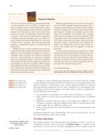
REVISITING
ommerce grew slowly at first, adding a few
branches each year, and its service became a
draw for the small-business customers on the lending
side. By 1994, Commerce had pioneered Sunday banking,
opening branches from 11 a.m. to 4 p.m. That same year,
Mr. Hill took another page from the McDonald’s handbook
with the launch of Commerce University—modeled after
Hamburger U. at McDonald’s.
“We are different!” shouts John Manning, a training
manager at the facility, before a room full of students.
Classes cover everything from loan underwriting to counting
cash. Today’s course is called “Traditions,” which includes
basics such as answering the phone in a chirpy voice.
One by one, students stand behind a screen and practice
their greeting—“Hello! My name is Linda! How may I help
you?!”—while the rest of the class rates the effort.
In 1994, the same year Commerce set up its training
facility, legislators in Washington revised banking laws to
allow interstate mergers, spurring the growth of behemoths
such as Bank of America Corp., Bank One Corp. and First
Union. The top priority for these banks was to cut costs
and squeeze more profits out of merged operations. Often
that started with staff cuts, which hurt morale.

“It makes for a very insecure environment,” says Rita
O’Brien, a retired executive at a small engineering company
who used to bank at First Union, but switched because of
poor service and fees to Commerce. “That gets reflected
back to the customer.” Indeed, U.S. Transactions, a firm
that researches banking markets, found that 3 out of 10
retail customers of merged banks say the merger hurt
service. Most of those say they want to leave their bank.
Mr. Hill, seeing an opportunity to grow much faster,
started hammering on the service message. He billed
Commerce as “America’s Most Convenient Bank,” in an
effort to steal dissatisfied customers from rivals. He
advertised hours, honed teller service, and began paying
his branches $5,000 to divide among the staff each time
a rival branch nearby closes its doors.

C
kofamerica
.com


Chapter 10 Standard Costing
411
SOURCES
: Jathon Sapsford, “Local McBanker: A Small Chain Grows by Borrowing Ideas from Burger Joints—Jersey’s Commerce Bancorp Stretches Hours, Cuts Fees to Build
Volume—The Catch: Lower Interest,”
The Wall Street Journal
(May 17, 2000), p. A1; Corporate Profile Web site, (June 16, 2000).
For Commerce, the challenge now is to maintain
service while growing. The company spends $100,000

on marketing each new branch opening to create a
hometown feeling, and the event is a flashback to another
banking era. On a recent Saturday in the Philadelphia
suburb of Flourtown, the neighborhood slowly turned out
to pick up free Commerce cups and pens. A magician
twisted balloons, while a disk jockey spun oldies. There
was a raffle and free soft drinks and hot dogs. Wayne
Gomes, a Philadelphia Phillies relief pitcher, signed photos
for kids in Little League outfits.
With assets of $7 billion, Commerce is the largest
bank headquartered in southern New Jersey. Its retail
approach to banking uses chain concepts that feature
standardized facilities, standardized hours, standardized
service, and aggressive marketing. The consistent delivery
and reinforcement of this strategy for over 26 years has
built a brand that the consumer has accepted as truth.
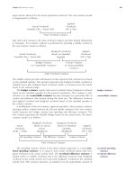
A standard cost is computed as a standard price multiplied by a standard quantity.
In a true standard cost system, standards are derived for prices and quantities of
each product component and for each product. A standard cost card provides in-
formation about a product’s standards for components, processes, quantities, and
costs. The material and labor sections of the standard cost card are derived from
the bill of materials and the operations flow document, respectively.
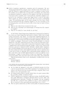
A variance is any difference between an actual and a standard cost. A total
variance is composed of a price and a usage subvariance. The material variances
are the price and the quantity variances. The material price variance can be com-
puted on either the quantity of material purchased or the quantity of material used
in production. This variance is computed as the quantity measure multiplied by the
difference between the actual and standard prices. The material quantity variance
is the difference between the standard price of the actual quantity of material used
and the standard price of the standard quantity of material allowed for the actual

output.
The two labor variances are the rate and efficiency variances. The labor rate
variance indicates the difference between the actual rate paid and the standard rate
allowed for the actual hours worked during the period. The labor efficiency vari-
ance compares the number of hours actually worked against the standard number
of hours allowed for the level of production achieved and multiplies this difference
by the standard wage rate.
If separate variable and fixed overhead accounts are kept (or if this information
can be generated from the records), two variances can be computed for both the
variable and fixed overhead cost categories. The variances for variable overhead
are the VOH spending and VOH efficiency variances. The VOH spending variance
is the difference between actual variable overhead cost and budgeted variable over-
head based on the actual level of input. The VOH efficiency variance is the dif-
ference between budgeted variable overhead at the actual activity level and vari-
able overhead applied on the basis of standard input quantity allowed for the
production achieved.
The fixed overhead variances are the FOH spending and volume variances.
The fixed overhead spending variance is equal to actual fixed overhead minus bud-
geted fixed overhead. The volume variance compares budgeted fixed overhead to
applied fixed overhead. Fixed overhead is applied based on a predetermined rate
using a selected measure of capacity. Any output capacity utilization actually achieved
(measured in standard input quantity allowed), other than the level selected to deter-
mine the standard rate, will cause a volume variance to occur.
CHAPTER SUMMARY
Depending on the detail available in the accounting records, a variety of over-
head variances may be computed. If a combined variable and fixed overhead rate
is used, companies may use a one-, two-, or three-variance approach. The one-
variance approach provides only a total overhead variance, which is the difference
between actual and applied overhead. The two-variance approach provides infor-
mation on a budget and a volume variance. The budget variance is calculated as

total actual overhead minus total budgeted overhead at the standard input quan-
tity allowed for the production achieved. The volume variance is calculated in the
same manner as under the four-variance approach. The three-variance approach
calculates an overhead spending variance, overhead efficiency variance, and a vol-
ume variance. The spending variance is the difference between total actual over-
head and total budgeted overhead at the actual level of activity worked. The effi-
ciency variance is the difference between total budgeted overhead at the actual
activity level and total budgeted overhead at the standard input quantity allowed
for the production achieved. The volume variance is computed in the same man-
ner as it was using the four-variance approach.
Actual costs are required for external reporting, although standard costs may
be used if they approximate actual costs. Adjusting entries are necessary at the end
of the period to close the variance accounts. Standards provide a degree of cleri-
cal efficiency and assist management in its planning, controlling, decision making,
and performance evaluation functions. Standards can also be used to motivate em-
ployees if the standards are seen as a goal of expected performance.
A standard cost system should allow management to identify significant vari-
ances as close to the time of occurrence as feasible and, if possible, to help de-
termine the variance cause. Significant variances should be investigated to decide
whether corrective action is possible and practical. Guidelines for investigation
should be developed using the management by exception principle.
Standards should be updated periodically so that they reflect actual economic
conditions. Additionally, they should be set at a level to encourage high-quality pro-
duction, promote cost control, and motivate workers toward production objectives.
Automated manufacturing systems will have an impact on variance computa-
tions. One definite impact is the reduction in or elimination of direct labor hours
or costs for overhead application. Machine hours, production runs, and number of
machine setups are examples of more appropriate activity measures than direct labor
hours in an automated factory. Companies may also design their standard cost sys-
tems to use only two elements of production cost: direct material and conversion.

Variances for conversion under such a system focus on machine or production ef-
ficiency rather than on labor efficiency.
Part 2 Systems and Methods of Product Costing
412
Mix and Yield Variances
Most companies use a combination of many materials and various classifications
of direct labor to produce goods. In such settings, the material and labor variance
computations presented in the chapter are insufficient.
When a company’s product uses more than one material, a goal is to combine
those materials in such a way as to produce the desired product quality in the most
cost-beneficial manner. Sometimes, materials can be substituted for one another
without affecting product quality. In other instances, only one specific material or
type of material can be used. For example, a furniture manufacturer might use
either oak or maple to build a couch frame and still have the same basic quality. A
perfume manufacturer, however, may be able to use only a specific fragrance oil
to achieve a desired scent.
APPENDIX
How do multiple material and
labor categories affect
variances?
7
Labor, like materials, can be combined in many different ways to make the
same product. Some combinations will be less expensive than others; some will be
more efficient than others. Again, all potential combinations may not be viable: Un-
skilled laborers would not be able to properly cut Baccarat or Waterford crystal.
Management desires to achieve the most efficient use of labor inputs. As with
materials, some amount of interchangeability among labor categories is assumed.
Skilled labor is more likely to be substituted for unskilled because interchanging
unskilled labor for skilled labor is often not feasible. However, it may not be cost
effective to use highly skilled, highly paid workers to do tasks that require little or

no training. A rate variance for direct labor is calculated in addition to the mix and
yield variances.
Each possible combination of materials or labor is called a mix. Management’s
standards development team sets standards for materials and labor mix based on
experience, judgment, and experimentation. Mix standards are used to calculate
mix and yield variances for materials and labor. An underlying assumption in prod-
uct mix situations is that the potential for substitution exists among the material
and labor components. If this assumption is invalid, changing the mix cannot im-
prove the yield and may even prove wasteful. In addition to mix and yield vari-
ances, price and rate variances are still computed for materials and labor. Consider
the following example.
The Fish Place has begun packaging a frozen one-pound “Gumbo-combo” that
contains processed crab, shrimp, and oysters. This new product is used to illus-
trate the computations of mix and yield variances. To some extent, one ingredient
may be substituted for the other. In addition, it is assumed that the company uses
two direct labor categories (A and B). There is a labor rate differential between
these two categories. Exhibit 10–11 provides standard and actual information for
the company for December 2000.
Material Price, Mix, and Yield Variances
A material price variance shows the dollar effect of paying prices that differ from
the raw material standard. The material mix variance measures the effect of
substituting a nonstandard mix of materials during the production process. The
Chapter 10 Standard Costing
413
mix
material mix variance
Material standards for one lot (200 1-pound packages):
Crab: 60 pounds at $7.20 per pound $ 432
Shrimp: 90 pounds at $4.50 per pound 405
Oysters: 50 pounds at $5.00 per pound 250

Total 200 pounds $1,087
Labor standards for one lot (200 1-pound packages):
Category A workers: 20 hours at $10.50 per hour $210
Category B workers: 10 hours at $14.30 per hour 143
Total 30 hours $353
Actual production and cost data for December:
Production: 40 lots
Material:
Crab: Purchased and used 2,285.7 pounds at $7.50 per pound
Shrimp: Purchased and used 3,649.1 pounds at $4.40 per pound
Oysters: Purchased and used 2,085.2 pounds at $4.95 per pound
Total 8,020.0 pounds
Labor:
Category A 903 hours at $10.50 per hour ($9,481.50)
Category B 387 hours at $14.35 per hour ($5,553.45)
Total 1,290 hours
EXHIBIT 10–11
Standard and Actual Information
for December 2000
material yield variance is the difference between the actual total quantity of in-
put and the standard total quantity allowed based on output; this difference re-
flects standard mix and standard prices. The sum of the material mix and yield
variances equals a material quantity variance similar to the one shown in the chap-
ter; the difference between these two variances is that the sum of the mix and
yield variances is attributable to multiple ingredients rather than to a single one.
A company can have a mix variance without experiencing a yield variance.
For Gumbo-combo, the standard mix of materials is 30 percent (60 pounds of
200 pounds per lot) crab, 45 percent shrimp, and 25 percent oysters. The yield of
a process is the quantity of output resulting from a specified input. For Gumbo-
combo, the yield from 60 pounds of crab, 90 pounds of shrimp, and 50 pounds of

oysters is one lot of 200 one-pound packages. Computations for the price, mix, and
yield variances are given below in a format similar to that used in the chapter:
Actual Mix ϫ Actual Mix ϫ Standard Mix ϫ Standard Mix ϫ
Actual Quantity Actual Quantity Actual Quantity Standard Quantity
ϫ Actual ϫ Standard ϫ Standard ϫ Standard
Price Price Price Price
Material Price Material Mix Material Yield
Variance Variance Variance
Assume The Fish Place used 8,020 total pounds of ingredients to make 40 lots of
Gumbo-combo. The standard quantity necessary to produce this quantity of Gumbo-
combo is 8,000 total pounds of ingredients. The actual mix of crab, shrimp, and
oysters was 28.5, 45.5, and 26.0 percent, respectively:
Crab (2,285.7 pounds out of 8,020) ϭ 28.5%
Shrimp (3,649.1 pounds out of 8,020) ϭ 45.5%
Oysters (2,085.2 pounds out of 8,020) ϭ 26.0%
Computations necessary for the material variances are shown in Exhibit 10–12.
These amounts are then used to compute the variances.
Part 2 Systems and Methods of Product Costing
414
material yield variance
yield
(1) Total actual data (mix, quantity, and prices):
Crab—2,285.7 pounds at $7.50 $17,142.75
Shrimp—3,649.1 pounds at $4.40 16,056.04
Oysters—2,085.2 pounds at $4.95 10,321.74 $43,520.53
(2) Actual mix and quantity; standard prices:
Crab—2,285.7 pounds at $7.20 $16,457.04
Shrimp—3,649.1 pounds at $4.50 16,420.95
Oysters—2,085.2 pounds at $5.00 10,426.00 $43,303.99
(3) Standard mix; actual quantity; standard prices:

Crab—30% ϫ 8,020 pounds ϫ $7.20 $17,323.20
Shrimp—45% ϫ 8,020 pounds ϫ $4.50 16,240.50
Oysters—25% ϫ 8,020 pounds ϫ $5.00 10,025.00 $43,588.70
(4) Total standard data (mix, quantity, and prices):
Crab—30% ϫ 8,000 pounds ϫ $7.20 $17,280.00
Shrimp—45% ϫ 8,000 pounds ϫ $4.50 16,200.00
Oysters—25% ϫ 8,000 pounds ϫ $5.00 10,000.00 $43,480.00
EXHIBIT 10–12
Computations for Material Mix
and Yield Variances
Actual M & Q; Standard M; Actual Standard M,
Actual M, Q, & P* Standard P Q; Standard P Q, & P
$43,520.53 $43,303.99 $43,588.70 $43,480.00
$216.54 U $284.71 F $108.70 U
Material Price Material Mix Material Yield
Variance Variance Variance
$40.53 U
Total Material Variance
*Note: M ϭ mix, Q ϭ quantity, and P ϭ price.
The above computations show a single price variance being calculated for materials.
To be more useful to management, separate price variances can be calculated for
each material used. For example, the material price variance for crab is $685.71 U
($17,142.75 Ϫ $16,457.04), for shrimp $364.91 F ($16,056.04 Ϫ $16,420.95), and
for oysters $104.26 F ($10,321.74 Ϫ $10,426.00). The savings on the shrimp and
oysters was less than the added cost for the crab, so the total price variance was
unfavorable. Also, less than the standard proportion of the most expensive ingre-
dient (crab) was used, so it is reasonable that there would be a favorable mix vari-
ance. The company also experienced an unfavorable yield because total pounds
of material allowed for output (8,000) was less than actual total pounds of material
used (8,020).

Labor Rate, Mix, and Yield Variances
The two labor categories used by The Fish Place are unskilled (A) and skilled (B).
When preparing the labor standards, the development team establishes the labor
categories required to perform the various tasks and the amount of time each task
is expected to take. During production, variances will occur if workers are not paid
the standard rate, do not work in the standard mix on tasks, or do not perform
those tasks in the standard time.
The labor rate variance is a measure of the cost of paying workers at other
than standard rates. The labor mix variance is the financial effect associated with
changing the proportionate amount of higher or lower paid workers in produc-
tion. The labor yield variance reflects the monetary impact of using more or
fewer total hours than the standard allowed. The sum of the labor mix and yield
variances equals the labor efficiency variance. The diagram for computing labor
rate, mix, and yield variances is as follows:
Actual Mix ϫ Actual Mix ϫ Standard Mix ϫ Standard Mix ϫ
Actual Hours ϫ Actual Hours ϫ Actual Hours ϫ Standard Hours ϫ
Actual Rate Standard Rate Standard Rate Standard Rate
Labor Rate Variance Labor Mix Variance Labor Yield Variance
Standard rates are used to make both the mix and yield computations. For
Gumbo-combo, the standard mix of A and B labor shown in Exhibit 10–11 is two-
thirds and one-third (20 and 10 hours), respectively. The actual mix is 70 percent
(903 of 1,290) A and 30 percent (387 of 1,290) B. Exhibit 10–13 presents the labor
computations for Gumbo-combo production. Because standard hours to produce
one lot of Gumbo-combo were 20 and 10, respectively, for categories A and B
labor, the standard hours allowed for the production of 40 lots are 1,200 (800 of
A and 400 of B). Using the amounts from Exhibit 10–13, the labor variances for
Gumbo-combo production in December are calculated in diagram form:
Chapter 10 Standard Costing
415
labor mix variance

labor yield variance
Standard M;
Actual M & H; Actual H;
Actual M, H, & R* Standard R Standard R Standard M, H, & R
$15,034.95 $15,015.60 $15,179.00 $14,120.00
$19.35 U $163.40 F $1,059 U
Labor Rate Labor Mix Labor Yield
Variance Variance Variance
$914.95 U
Total Labor Variance
*Note: M ϭ mix, H ϭ hours, and R ϭ rate.
As with material price variances, separate rate variances can be calculated for
each class of labor. Because category A does not have a labor rate variance, the
total rate variance relates to category B.
The company has saved $163.40 by using the actual mix of labor rather than
the standard. A higher proportion of the less expensive class of labor (category A)
than specified in the standard mix was used. One result of substituting a greater
proportion of lower paid workers seems to be that an unfavorable yield occurred
because total actual hours (1,290) were greater than standard (1,200).
Because there are trade-offs in mix and yield when component qualities and
quantities are changed, management should observe the integrated nature of price,
mix, and yield. The effects of changes of one element on the other two need to
be considered for cost efficiency and output quality. If mix and yield can be in-
creased by substituting less expensive resources while still maintaining quality, man-
agers and product engineers should change the standards and the proportions of
components. If costs are reduced but quality maintained, selling prices could also
be reduced to gain a larger market share.
Part 2 Systems and Methods of Product Costing
416
(1) Total actual data (mix, hours, and rates):

Category A—903 hours at $10.50 $9,481.50
Category B—387 hours at $14.35 5,553.45 $15,034.95
(2) Actual mix and hours; standard rates:
Category A—903 hours at $10.50 $9,481.50
Category B—387 hours at $14.30 5,534.10 $15,015.60
(3) Standard mix; actual hours; standard rates:
Category A—2/3 ϫ 1,290 ϫ $10.50 $9,030.00
Category B—1/3 ϫ 1,290 ϫ $14.30 6,149.00 $15,179.00
(4) Total standard data (mix, hours, and rates):
Category A—2/3 ϫ 1,200 ϫ $10.50 $8,400.00
Category B—1/3 ϫ 1,200 ϫ $14.30 5,720.00 $14,120.00
EXHIBIT 10–13
Computations for Labor Mix and
Yield Variances
KEY TERMS
bill of material (p. 383)
budget variance (p. 397)
controllable variance (p. 397)
expected standard (p. 405)
fixed overhead spending variance (p. 395)
flexible budget (p. 392)
Chapter 10 Standard Costing
417
ideal standard (p. 406)
labor efficiency variance (p. 392)
labor mix variance (p. 415)
labor rate variance (p. 392)
labor yield variance (p. 415)
material price variance (p. 389)
material quantity variance (p. 391)

material mix variance (p. 413)
material yield variance (p. 414)
mix (p. 413)
noncontrollable variance (p. 395)
normal capacity (p. 392)
operations flow document (p. 385)
overhead efficiency variance (p. 397)
overhead spending variance (p. 397)
practical capacity (p. 392)
practical standard (p. 405)
standard cost (p. 382)
standard cost card (p. 386)
standard quantity allowed (p. 389)
theoretical capacity (p. 392)
total overhead variance (p. 396)
total variance (p. 387)
variable overhead efficiency variance
(p. 395)
variable overhead spending variance
(p. 394)
variance analysis (p. 402)
volume variance (p. 395)
yield (p. 414)
Actual Costs
Direct Material: Actual Price ϫ Actual Quantity Purchased or Used
DM: AP ϫ AQ ϭ AC
Direct Labor: Actual Price (Rate) ϫ Actual Quantity of Hours Worked
DL: AP ϫ AQ ϭ AC
Standard Costs
Direct Material: Standard Price ϫ Standard Quantity Allowed

DM: SP ϫ SQ ϭ SC
Direct Labor: Standard Price (Rate) ϫ Standard Quantity of Hours Allowed
DL: SP ϫ SQ ϭ SC
Standard Quantity Allowed: Standard Quantity of Input (SQ) ϫ Actual Quantity
of Output Achieved
Variances in Formula Format
The following abbreviations are used:
AFOH ϭ actual fixed overhead
AM ϭ actual mix
AP ϭ actual price or rate
AQ ϭ actual quantity or hours
AVOH ϭ actual variable overhead
BFOH ϭ budgeted fixed overhead (remains at constant amount regardless of
activity level as long as within the relevant range)
SM ϭ standard mix
SP ϭ standard price
SQ ϭ standard quantity
TAOH ϭ total actual overhead
Material price variance ϭ (AP ϫ AQ) Ϫ (SP ϫ AQ)
Material quantity variance ϭ (SP ϫ AQ) Ϫ (SP ϫ SQ)
Labor rate variance ϭ (AP ϫ AQ) Ϫ (SP ϫ AQ)
Labor efficiency variance ϭ (SP ϫ AQ) Ϫ (SP ϫ SQ)
SOLUTION STRATEGIES
Four-variance approach:
Variable OH spending variance ϭ AVOH Ϫ (VOH rate ϫ AQ)
Variable OH efficiency variance ϭ (VOH rate ϫ AQ) Ϫ (VOH rate ϫ SQ)
Fixed OH spending variance ϭ AFOH Ϫ BFOH
Volume variance ϭ BFOH Ϫ (FOH rate ϫ SQ)
Three-variance approach:
Spending variance ϭ TAOH Ϫ [(VOH rate ϫ AQ) ϩ BFOH]

Efficiency variance ϭ [(VOH rate ϫ AQ) ϩ BFOH)] Ϫ [(VOH rate ϫ SQ) ϩ BFOH]
Volume variance ϭ [(VOH rate ϫ SQ) ϩ BFOH] Ϫ [(VOH rate ϫ SQ) ϩ
(FOH rate ϫ SQ)] (This is equal to the volume variance of the
four-variance approach.)
Two-variance approach:
Budget variance ϭ TAOH Ϫ [(VOH rate ϫ SQ) ϩ BFOH]
Volume variance ϭ [(VOH rate ϫ SQ) ϩ BFOH] Ϫ [(VOH rate ϫ SQ) ϩ
(FOH rate ϫ SQ)] (This is equal to the volume variance of the
four-variance approach.)
One-variance approach:
Total OH variance ϭ TAOH Ϫ (Combined OH rate ϫ SQ)
MULTIPLE MATERIALS:
Material price variance ϭ (AM ϫ AQ ϫ AP) Ϫ (AM ϫ AQ ϫ SP)
Materials mix variance ϭ (AM ϫ AQ ϫ SP) Ϫ (SM ϫ AQ ϫ SP)
Materials yield variance ϭ (SM ϫ AQ ϫ SP) Ϫ (SM ϫ SQ ϫ SP)
MULTIPLE LABOR CATEGORIES:
Labor rate variance ϭ (AM ϫ AQ ϫ AP) Ϫ (AM ϫ AQ ϫ SP)
Labor mix variance ϭ (AM ϫ AQ ϫ SP) Ϫ (SM ϫ AQ ϫ SP)
Labor yield variance ϭ (SM ϫ AQ ϫ SP) Ϫ (SM ϫ SQ ϫ SP)
VARIANCES IN DIAGRAM FORMAT:
Direct Materials and Direct Labor
Actual Price ϫ Standard Price ϫ
Actual Quantity Purchased Actual Quantity Purchased
Material Price Variance
Standard Price ϫ Standard Price ϫ
Actual Quantity Used Standard Quantity Allowed
Material Quantity Variance
Actual Price ϫ Standard Price ϫ Standard Price ϫ
Actual Quantity Used Actual Quantity Used Standard Quantity Allowed
Material Price Variance Material Quantity Variance

Total Material Variance
Part 2 Systems and Methods of Product Costing
418
Actual Price ϫ Standard Price ϫ Standard Price ϫ
Actual Quantity of Actual Quantity of Standard Quantity of
Hours Worked Hours Worked Hours Allowed
Labor Rate Variance Labor Efficiency Variance
Total Labor Variance
Overhead four-variance approach:
Variable Overhead
Applied VOH
Actual VOH VOH Rate ϫ Actual Quantity VOH Rate ϫ Standard Quantity
(a) (b)
VOH Spending Variance VOH Efficiency Variance
Total Variable OH Variance
Fixed Overhead
Applied FOH
Actual FOH Budgeted FOH FOH Rate ϫ Standard Quantity
(c) (d)
FOH Spending Variance Volume Variance
Total Fixed OH Variance
Overhead one-, two-, and three-variance approaches:
Budget Based Budget Based
Actual on Input Hours on Output Hours Applied
Actual VOH VOH Rate ϫ AQ VOH Rate ϫ SQ VOH Rate ϫ SQ
ϩ Actual FOH ϩ Budgeted FOH ϩ Budgeted FOH ϩ FOH Rate ϫ SQ
(a) ϩ (c) (b) (d)
Spending Variance Efficiency Variance Volume Variance
(a) ϩ (b) ϩ (c) (d)
Budget Variance Volume Variance

(a) ϩ (b) ϩ (c) ϩ (d)
Total Overhead Variance
(Total Under/Overapplied Overhead)
Mix and Yield Variances
MULTIPLE MATERIALS:
Actual Mix ϫ Actual Mix ϫ Standard Mix ϫ Standard Mix ϫ
Actual Quantity Actual Quantity Actual Quantity Standard Quantity
ϫ Actual Price ϫ Standard Price ϫ Standard Price ϫ Standard Price
Material Price Variance Material Mix Variance Material Yield Variance
MULTIPLE LABOR CATEGORIES:
Actual Mix ϫ Actual Mix ϫ Standard Mix ϫ Standard Mix ϫ
Actual Hours ϫ Actual Hours ϫ Actual Hours ϫ Standard Hours ϫ
Actual Rate Standard Rate Standard Rate Standard Rate
Labor Rate Variance Labor Mix Variance Labor Yield Variance
Chapter 10 Standard Costing
419
Part 2 Systems and Methods of Product Costing
420
Poly Containers makes 300-gallon plastic water tanks for a variety of commercial
uses. The standard per unit material, labor, and overhead costs are as follows:
Direct material: 80 pounds @ $2 $160
Direct labor: 1.25 hours @ $16 per hour 20
Variable overhead: 30 minutes of machine time @ $50.00 per hour 25
Fixed overhead: 30 minutes of machine time @ $40.00 per hour 20
The overhead application rates were developed using a practical capacity of 6,000
units per year. Production is assumed to occur evenly throughout the year.
During May 2001, the company produced 525 tanks. Actual data for May 2001
are as follows:
Direct material purchased: 46,000 pounds @ $1.92 per pound
Direct material used: 43,050 pounds (all from May’s purchases)

Total labor cost: $10,988.25 for 682.5 hours
Variable overhead incurred: $13,770 for 270 hours of machine time
Fixed overhead incurred: $10,600 for 270 hours of machine time
Required:
Calculate the following:
a. Material price variance based on purchases
b. Material quantity variance
c. Labor rate variance
d. Labor efficiency variance
e. Variable overhead spending and efficiency variances
f. Fixed overhead spending and volume variances
g. Overhead variances using a three-variance approach
h. Overhead variances using a two-variance approach
i. Overhead variance using a one-variance approach
Solution to Demonstration Problem
a.
AP ϫ AQ
p
SP ϫ AQ
p
$1.92 ϫ 46,000 $2.00 ϫ 46,000
$88,320 $92,000
$3,680 F
MPV
b. SQ ϭ 525 ϫ 80 pounds ϭ 42,000 pounds
SP ϫ AQ
u
SP ϫ SQ
$2 ϫ 43,050 $2 ϫ 42,000
$86,100 $84,000

$2,100 U
MQV
c. & d. AR ϭ $10,988.25 Ϭ 682.5 hours ϭ $16.10 per hour
SQ ϭ 525 ϫ 1.25 hours ϭ 656.25 hours
AP ϫ AQ SP ϫ AQ SP ϫ SQ
$16.10 ϫ 682.5 $16 ϫ 682.5 $16 ϫ 656.25
$10,988.25 $10,920 $10,500
$68.25 U $420 U
LRV LEV
DEMONSTRATION PROBLEM
e. SQ ϭ 525 ϫ 0.5 ϭ 262.5 hours
SP ϫ AQ SP ϫ SQ
Actual VOH $50.00 ϫ 270 $50.00 ϫ 262.5
$13,770 $13,500 $13,125
$270 U $375 U
VOH Spending Variance VOH Efficiency Variance
f. BFOH, annually ϭ 6,000 ϫ $20 ϭ $120,000
BFOH, monthly ϭ $120,000 Ϭ 12 months ϭ $10,000
SQ ϭ 262.5 hours [from part (e)].
SP ϫ SQ
Actual FOH Budgeted FOH $40 ϫ 262.50
$10,600 $10,000 $10,500
$600 U $500 F
FOH Spending Variance Volume Variance
g., h., and i. Combined overhead application rate ϭ $50 ϩ $40 ϭ $90 per MH;
SQ ϭ 262.5 hours [from part (e)].
Actual VOH VOH Rate ϫ AQ VOH Rate ϫ SQ Applied OH
ϩ Actual FOH ϩ Budgeted FOH ϩ Budgeted FOH (SP ϫ SQ)
$13,770 $50 ϫ 270 ϭ $13,500 $50 ϫ 262.5 ϭ $13,125 $50 ϫ 262.5 ϭ $13,125
ϩ 10,600 ϩ 10,000 ϩ 10,000 ϩ 40 ϫ 262.5 ϭ 10,500

$24,370 $23,500 $23,125 $90 ϫ 262.5 ϭ $23,625
$870 U $375 U $500 F
Spending Variance Efficiency Variance Volume Variance
VOH Rate ϫ SQ
ϩ Budgeted FOH
$50 ϫ 262.50 ϭ $13,125 Applied OH
Actual OH ϩ 10,000 (SP ϫ SQ)
$24,370 $23,125 $90 ϫ 262.50 ϭ $23,625
$1,245 U $500 F
Budget Variance Volume Variance
Applied OH
Actual OH SP ϫ SQ
$24,370 $90 ϫ 262.50 ϭ $23,625
$745 U
Total Overhead Variance
(Total Under/Overapplied Overhead)
Chapter 10 Standard Costing
421
1. What are the three primary uses of a standard cost system? In a business that
routinely manufactures the same products or performs the same services, why
would standards be helpful?
2. The standards development team should be composed of what experts? Why
are these people included?
3. Discuss the development of standards for a material. How is the quality stan-
dard established for a material?
QUESTIONS