Báo cáo hóa học: " Performance analysis of spectrum sharing mechanisms in cognitive radio networks" pptx
Bạn đang xem bản rút gọn của tài liệu. Xem và tải ngay bản đầy đủ của tài liệu tại đây (558.06 KB, 15 trang )
RESEARCH Open Access
Performance analysis of spectrum sharing
mechanisms in cognitive radio networks
Chen Peipei, Zhang Qinyu
*
, Zhang Yalin and Wang Ye
Abstract
In this article, a non-preemptive (NP) mechanism is proposed to improve the quality-of-service (QoS) of secondary
users (SUs) in joint leasing and sensing-based cognitive radio networks (CRNs). In this spectrum-sharing mechanis m,
a primary user (PU) could not forcibly terminate a SU with ongoing transmission. Both the typical preemptive and
the proposed NP mechanisms are modeled by multi-dimensional Markov chains with three state variables. A
decomposition-approximated method is used to derive the closed-form solutions of the steady-state probabilities in
the Markov chains. The analytical results are verified by numerical results. System parameters that affect performance
metrics are also investigated in these two mechanisms. The simulation results show that in the proposed mechanism
the performance metrics of SUs such as force-termination probability and mean system delay are improved
significantly, with an acceptable loss of PUs’ QoS in terms of mean waiting time and blocking probability. A QoS
tradeoff can be achieved between the primary and the secondary systems. For QoS improvement of SUs, the
proposed NP mechanism outperforms the preemptive mechanism in joint leasing and sensing-based CRNs.
Keywords: cognitive radio networks, joint leasing and sensing, non-preemptive mechanism, QoS tradeoff
1. Introduction
Cognitive radio (CR) has been c onsidered as a viable
technique to improve the uti lization of spectral resources
in a li censed (primary) system [1]. The secondary users
(SUs) in the unlice nsed (se condary) system are allowed
to opportunistically utilize the spectrum holes that are
temporarily unoccupied by primary users (PUs). The key
enabler is the SU with CR technology, which can sense
the spectrum hole and accordingly adjust its transmission
parameters. The main idea of CR is that SUs exploit the
spectrum holes and take advantage of them opportunisti-
cally. Therefore, the spectrum sharing mechanism in CR
networks (CRNs) becomes a hot research topic.
According t o t he literature related to CRNs, previous
study on dynamic spectrum access (DSA) can be categor-
ized as sensing-based access model , leasing-based access
model, and joint leasing and sensing-based access model.
In sensing-based CRNs [2-5], SUs acquire the information
of spe ctrum holes through spectrum sensing and freely
access the unoccupied licensed channels, without paying
any leasing fees to primary system. The primary system is
ignorant of SUs, and the quality-of-service (QoS) of PUs
should be protected by a specific spectrum sharing
mechanism. In leasing-based CRNs [6], the secondary sys-
tem dynamically leases spectrum from primary system and
owns exclusive right to access the le ased spectrum. How-
ever, the spectrum leasing is not performed in re al time
and the SUs will keep the exclusive right until the lease
term expires, which may cause a great QoS degradation to
primary system once the PUs’ services grow abruptly. The
joint leasing and sensing-based CRN proposed in [7] is
widely considered to be a viable market option that bene-
fits both the primary and the secondary systems. The pri-
mary system can make extra profit via spectrum leasing
(unlike in sensing-based CRNs) and SUs have full flexibil-
ity in utilizing the spectrum holes (unlike in leasing-based
CRNs). SUs pay the primary system the channel leasing
fees only for opportunistic access. The joint leasing and
sensi ng-based model enables more flexible integration of
DSA in the licensed spectrum via real-time spectrum
leasing.
In this article, we study the spectrum-sharing mechan-
isms in joint leasing and sensing-based CRNs, which ben-
efit both the primary and the secondary systems. The
authors in [8] proposed a preemptive spectrum-sharing
* Correspondence:
Department of Electronic and Information Engineering, Shenzhen Graduate
School, Harbin Institute of Technology, Shenzhe n, China
Peipei et al. EURASIP Journal on Wireless Communications and Networking 2011, 2011:129
/>© 2011 Peipei et al; licensee Springer. Thi s is an Open Access article distributed under the terms of the Creative Commons Attribution
License (http://creativecomm ons.org/licenses/by/2.0), which permits unrestricted use, distribution, and repr oduction in any medium,
provided the original work is properly cited.
mechanism in joint leasing and sensing-based CRNs.
This preemptive mechanism is the same as the traditional
spectrum-sharing mechanism in sensing-based CRNs
[2-5], which has the basic requirementthatthePUsare
not affected by the SUs’ opportunistic spectrum utiliza-
tion. A SU has to vacate the channel p romptly when a
PU returns and handoff to another spectrum hole. When
no spectrum hol e is available, the SU’s ongoing transmis-
sion is terminated and the SU is preempted. In the pre-
emptive mechanism, PUs have preemptive priorities over
SUs. The preemptive mechanism causes significant force-
termination probability for SUs [2]. That is not only a
waste of r esources (power and frequency), but also insuf-
ferable for SUs, especially for the SUs who lease spectrum
for some guarantees of QoS. We originally present a non-
preemptive (NP) spectrum-sh aring mechanis m, in which
PUs have no preemptive priorities over SUs. A PU would
wait for a period of time until the completion of the SU’s
ongoing transmission when no spectrum hole is available.
No SU would forcibly be terminated by PUs. A QoS tra-
deoff will be achieved between the primary and the sec-
ondary systems. We focus on the performance analysis of
spectrum-sharing mechanisms, which not only gives the
evaluation of the spectrum-shar ing mechanisms, but also
provides a clue for future rese arches on strategies o f pri-
mary and secondary systems in joint leasing and sensing-
based CRNs.
The interactions between PUs and SUs i n spectrum
sharing can be modeled b y a multi-dimensional Markov
chain. For comparison, both the preemptive and the NP
mechanisms are modeled based on the Markov process.
Markov theory is an effective metho d to model the spec-
trum sharing in CR systems [2,3, 5]. However, it is always
non-trivial to obtain the exact closed-form solutions of the
steady-state probabilities. An approximate method intro-
duced by Ghain and Schwartz [9,10] can be used for ana-
lyzing the Markov chain and deducing the approximate
closed-form solutions of steady-state probabilities since we
suppose that the SUs have much shorter average service
time than PUs. Performance metrics such as mean system
delay and force-termination probability of SU, average
waiting time, and blocking probability of PU are evaluated
with the steady-state probabilities in CRNs. The QoS tra-
deoff relationships between primary and secondary sys-
tems are discussed. In addition, the influences of system
parameters on performance metrics have also been
presented.
This rest of the article is organized as follows. In Sec-
tion 2, we first present the system model of a joint leasing
and sensing-base d CRN, and introduce the preemptive
and the NP mechanisms based on three-dimensional
Markov chains. We then derive the closed-form solutions
of the steady-state probabilities in the Markov chains by
decomposition approximation. In Sectio n 3, we give the
expressions of performance metrics. To verify the analyti-
cal solution, simulation results are carried o ut and the
two spectrum-sha ring mechanisms are compared and
discussed in Section 4. Finally, conclusion is drawn in
Section 5.
2. System model
The joint leasing and sensing-based access model can be
described as a CRN with three interacting layers [7]: pri-
mary system (with PU access point and PUs), spectrum
broker, and secondary system (with SU access point and
SUs with CR capabilities). The system model is depicted
in Figure 1. The primary system divides the licensed
spectrum into two parts. One part consists of reserved
channels for PUs transmission only, and the other part
consists of the shared channels that can be used by SUs
opportunistically. The primary system can temporarily
lease its spectrum usage rights of the shared channels to
secondary system through the spectrum broker, and get
payoff from secondary system as SUs opportunistically
utilize the shared channels. The spectrum broker can be
either a regulatory authority (e.g., FCC in USA, Ofcom in
UK) or an authorized third-party. The spectrum broker
works as an interaction entity between the primary and
the secondary s ystems [11 ]. A contract between the pri-
mary and t he secondary systems has to be made in spec-
trum broker. The interactions between the primary and
the secondary systems in a three-tier CRN can be mod-
eled by a Stackelberg game [12], where the primary sys-
tem is the leader and secondary system is the follower.
The leader announces its own policies (the range of
shared channel s, spectrum leasing cost), and the second-
ary system makes its own decisions (the range of leased
channels, service tariff) with the knowledge of the leader’s
decisions. The primary and the secondary systems
exchange their information through spectrum broker.
For simplicity, we assume that there are one primary sys-
tem and one secondary system. In this joint leasing and
sensing-based three-tier CRN, the spectrum-sharing
mechanism has the major influences on the primary and
the secondary systems’ decisions. The economic factor is
not our focus here and will be considered in our f uture
research.
We ass ume that there are N licensed channels in a pri -
mary system, and each of them has identical bandwidth.
Among these N channels, R channels are dedicated for
PUs, and N - R channelsaresharedbyPUsandSUs.A
SU can sense the shared chan nels by spectrum sensing
and access the channel if it i s not occupied by a PU. The
PU and the SU arrival processes follow Poisson process
with arrival rates l
p
and l
s
, respectively. The service in
the CRN is a single-slot first c ome first served transmis-
sion. The service time of the PU follows exponential dis-
tribution with mean 1/μ
p
and that of the SU follows
Peipei et al. EURASIP Journal on Wireless Communications and Networking 2011, 2011:129
/>Page 2 of 15
exponential distribution with mean 1/μ
s
.Asthenumber
of spectrum holes varies with PUs traffic dram atically, we
assume the traffic of SUs has much shorter a verage ser-
vice time compared to the traffic of PUs. A first in first
out buffer of size Q is allocated for the secondary system.
In this section, we describe the process of spectrum
sharing in the CRN as a multi-dimensional Markov
chain with three state variables. The states in the model
are denoted as
N
p
(
t
)
, N
s
(
t
)
, N
s
(
t
)
.
P
i,j,k
= lim
t→∞
P
N
p
(
t
)
= i, N
’
s
(
t
)
= j, N
s
(
t
)
= k
repre-
sents the steady probability of state, in which N
p
(t)=i
is the number of PUs in the system,
N
s
(
t
)
=
j
is the
number of SUs in the system, N
s
(t)=k is the number of
SUs in service. Here, we use (i, j, k)asthenotationofa
state in the model.
2.1 Preemptive mechanism
In the preemptive mechanism, a SU has to switch to
another spectrum hole or stop its transmission (be pre-
empted) as soon as a PU reclaims the channel, since
PUs are given priorities over SUs. The pr eempted SU
that ceases ongoing packet transmission will put the
failed transmission packet into the buffer and wait for
transmission again. However, if the buffer is full, then
the SU’s failed transmission packet will be dropped. The
number of channels that SUs can use is a random vari-
able, which depends on the PUs’ service probability dis-
tributions. Since the number of the spectrum holes
depends on the PUs’ traffic, the number of S Us in ser-
vice also varies with PUs’ traffic. Figure 2 shows an
example of the state transition diagram with N =3,R =
1. The state space of the preemptive mechanism Ω
pre
is
presented as
pre
=
⎧
⎪
⎨
⎪
⎩
i, j, k
:0≤ i ≤ N;0 ≤ k ≤ min
(
N − R, N − i
)
;
j = k,if0≤ k < min
(
N − R, N − i
)
;
k ≤ j ≤ k + Q,ifk = min
(
N − R, N − i
)
⎫
⎪
⎬
⎪
⎭
.
In F igure 2, we can see that unidirectional transitions
exist in the Markov chain, so that the Markov chain
cannot be reversible, which means that the exact closed-
form solutions are non-tri vial to obtain. Decomposit ion
technique [9] is used as a tool to derive the approximate
close d-form solutions of steady-state probab ilities in the
Markov chain. The Markov chain can be broken down
into a hierarchy of groups of a ggregate states. Each
group of states comprises of all the states with a fixed
number of PUs. Figure 2 shows that there are four
groups of aggregate states and each group is circled by a
line separately. All transitions between the groups are in
terms of l
p
and μ
p
.Forthedurationofaspecificnum-
ber of PUs, the states of SUs achieve equilibrium. All
the transitions within a group are in terms of l
s
and μ
s
,
and the steady-state probabilities
P
pre
i,
j
,k
in the preemptive
mechanism can be approximated by ignoring the transi-
tions between groups.
PUs have preemptive priorities over SUs, which
implies that the equilibrium distribution of PUs can
simplybemodeledasaM/M/N/N queueing system. P
i
represents the probability of i PUs in the system, which
can be derived by Erlang-B formula [9]:
P
i
=
ρ
i
p
i!
N
j=0
ρ
j
p
j!
,whereρ
p
=
λ
p
μ
p
.
(1)
Spectrum
Broker
12
Reserved channels for PUs
Shared Channels can be used by SUs
opportunistically
RR+1
1
S
U system
Figure 1 System model.
Peipei et al. EURASIP Journal on Wireless Communications and Networking 2011, 2011:129
/>Page 3 of 15
∀
i
Î {0,1, ,R}, the M/M/N-R/N-R+Q queueing sys-
tem can be used to obtain
P
pre
i,j,min
(
j,N−R
)
, which repre-
sents the probability of j SUs in the system. r
s
= l
s
/μ
s
refers to the SU traffic load in Erlang. For simplicity, we
denote N-R = D, N-R+Q = E.
P
pre
i,j,min
(
j,D
)
=
⎧
⎪
⎨
⎪
⎩
P
i
· P
pre
i,0
ρ
j
s
j!0≤ j <
D
P
i
·
P
pre
i,0
ρ
j
s
D
!
D
j−D
D ≤ j ≤ E
(2)
P
pre
i,0
=
⎛
⎜
⎝
ρ
D
s
1 −
ρ
s
D
(Q+1)
1 −
ρ
s
D
D!
+
D−1
x=0
ρ
x
s
x!
⎞
⎟
⎠
−
1
(3)
∀
i
Î {R+1, , N-1},
P
pre
i,j,min
(
j,N−i
)
can be derived from
the M/M/N-i/N-i+Q queueing system similarly as (2)
and (3).
For i = N, we construct the balance equations of the
states in the group. The steady-state probabilities can be
easily obtained.
P
pre
N,
j
,0
= λ
j
s
P
pre
N,0,
0
(4)
Q
j
=0
P
pre
N,j,0
=
1+λ
s
+ ···+ λ
Q
s
P
pre
N,0,0
= P
N
(5)
All the steady-state probabilities in the preemptive
mechanism are given approximately in above formulas.
The complete algorithm for the steady-state probabilities
in the preemptive mechanism is described in Appendix
A
2.2. NP mechanism
In the NP mechanism, PUs have no preemptive priori-
ties over SUs. When there is no spectrum hole to
switc h, a SU would not vacate the channel reclaimed by
a PU until the SU finishes its ongoing transmission. It
means that SUs would not be forcibly terminated by
PUs. Both the primary and the secondary systems can
communicate with the spectrumbrokerthroughauxili-
ary control chan nels [7]. We descri be the explicit inter-
actions between the primary and the secondary systems
as follows.
In the secondary system, SUs can monitor the real-
time situation of the shared channels by periodic spec-
trum sensing. Once there is no spectrum hole, the sec-
ondary system will inform a waiting signaling to the
primary system through the spect rum broker. After
0,1,1
0, 2, 2
p
O
p
P
0, 0, 0
0, 3, 2
0, 4, 2
s
P
s
O
s
O
s
O
s
O
2
s
P
2
s
P
2
s
P
p
O
p
P
p
O
p
P
p
O
p
P
p
O
p
P
1,1,1
1, 2, 2
1, 0, 0
1, 3, 2
1, 4, 2
s
P
s
O
s
O
s
O
s
O
2
s
P
2,1,1
2, 2,1
2, 0, 0
2,3,1
s
P
s
O
s
O
s
O
2
p
P
p
O
2
p
P
p
O
2
p
P
p
O
2
p
P
p
O
p
O
3,1, 0
3, 2, 0
3, 0, 0
s
O
s
O
3
p
P
p
O
3
p
P
p
O
p
O
3
p
P
p
O
s
P
s
P
2
s
P
2
s
P
Figure 2 An example of the preemptive mechanism.
Peipei et al. EURASIP Journal on Wireless Communications and Networking 2011, 2011:129
/>Page 4 of 15
receiving this signaling, the PU who is ready to transmit
will wait for a period of time and inform the secondary
system the target channel that it reclaims. The SU in
the specific channel will vacate the channel immediately
after it finish es the ongoing transmission. If the channel
can be released before the PU’ s waiting time is due,
then the PU can access the target channel and the PU’s
serviceisonlydeferred.Otherwise,thePUwillbe
blocked. Once the SUs sense that there appears a spec-
trum hole (a SU or PU in service left), the waiting sig-
naling is canceled for PUs in the primary system via the
spectrum broker. In the situation without waiting signal-
ing, the proposed mechanism works in the same way as
the preemptive mechanism.
In this article, we assume that the waiting time of a
PU follows exponential distribution with mean 1/μ
p
,
which is the same as the PU’s service time. Therefore,
the total rate of a PU leaving the system only depends
on N
p
(t). This implies that the number of PUs in the
system is independent of the SUs’ traffic and the steady
state probabilities of N
p
(t) can also be derived by (1).
Figure 3 shows an example of the state transition dia-
gram of NP mechanism with N =3,R=1.Thestate
space of NP mechanism Ω
nonpre
is
nonpre
=
⎧
⎪
⎪
⎪
⎪
⎨
⎪
⎪
⎪
⎪
⎩
S
n
=
pre
S
q
=
⎧
⎪
⎨
⎪
⎩
i, j, k
: R +1≤ i ≤ N;
min
(
N − i, N − R
)
< k ≤ max
(
N − i, N − R
)
;
k ≤ j ≤ k + Q
⎫
⎪
⎬
⎪
⎭
⎫
⎪
⎪
⎪
⎪
⎬
⎪
⎪
⎪
⎪
⎭
.
In Figure 3, the shaded states represent the states with
PUs queueing for transmission, and these states do not
exist in preemptive mechanism. The set of states with
PUs queueing is denoted as S
q
, while the set of the
other states in Ω
nonpre
is denoted as S
n
.Inqueueing
states, i+k >N, only N-K PUs ar e in service, i-(N-K)PUs
are queueing for transmission.
We use the decomposition technique to derive the
appr oximate closed-form solutions of steady-state prob-
abilities
P
nonpre
i,
j
,k
in the proposed NP mechanism.
Step 1. For i Î (0, , R), all states are in S
n
,andthe
state transitions in each group can be modeled as M/M/
0, 0,0
0,1,1 0, 2, 2
0,3, 2
0, 4, 2
1, 0, 0
1, 1, 1
1, 2, 2
1, 3, 2
1, 4, 2
2, 0,0 2,1,1
2, 2,1
2,3,1
3, 0, 0
3,1, 0
3, 2, 0
2, 2, 2
2,3,2
2, 4, 2
3, 2, 2
3, 3, 2
3, 4, 2
3,1,1
3, 2,1
3, 3,1
s
O
s
O
s
O
s
O
s
P
2
s
P
2
s
P
2
s
P
s
P
2
s
P
2
s
P
2
s
P
s
O
s
O
s
O
s
O
p
O
p
O
p
O
p
O
p
O
p
P
p
P
p
P
p
P
p
P
s
O
s
O
s
O
s
P
s
P
s
P
s
O
s
O
p
O
p
O
p
O
2
p
P
2
p
P
2
p
P
2
p
P
s
P
s
P
s
P
s
O
s
O
3
p
P
s
O
s
O
p
O
p
O
p
O
2
p
P
2
p
P
2
p
P
2
s
P
2
s
P
2
s
P
3
p
P
3
p
P
3
p
P
p
O
p
O
p
O
s
O
s
O
2
s
P
2
s
P
2
s
P
p
O
3
p
P
3
p
P
3
p
P
p
O
p
O
3
p
P
3
p
P
Non-queueing state in
Queueing state in
n
S
q
S
Figure 3 An example of the non-preemptive mechanism.
Peipei et al. EURASIP Journal on Wireless Communications and Networking 2011, 2011:129
/>Page 5 of 15
(N-R)/(N-R)+Q . Therefore, the steady-state probabilities
of j SUs in the system
P
nonpre
i,j,min
(
j,N−R
)
can be derived by
the same formulas as (2) and (3).
Step 2. For i Î (R, , N-1), we denote the queueing
states as (i’,j,k) to distinguish it from the non-queueing
states here. The transitions into the queuei ng states {i =
1 ≤ i’ ≤ N, j ≤ k, k =min(N-i, N-R)}areonlyfromthe
non-queueing states {i, j ≤ k, k =min(N-i, N-R)}, which
have been obtained from last step. Figure 4 shows an
example of the transition diagram between non-queue-
ing states and queueing states.
We define the terms F
i, j, k
, R
i, j, k
as follows.
F
i
,j,k
≡ P
nonpre
i
,j−1,k
λ
s
ϕ
i
, j − 1, k
= total probability flux into state
i
, j, k
other than from
i
− 1, j, k
or
i
+1,j,k
(6)
in which (i’ ,j,k) indicates whether the state (i’ ,j,k)
exists or not, i.e. (i’,j,k) = 1, if (i’,j,k) Î Ω
nonpre
.
R
i
,j,k
= λ
s
+ kμ
s
+ λ
p
+ i
μ
p
= total rate out of state
i
, j, k
.
(7)
We use (6) and (7) to construct balance equations for
the queueing states, as proposition 1 in [10].
P
nonpre
i,
j
,k
satisfies the following recursive relationship:
P
nonpre
i
,
j
,k
=
i
−1,j,k
+ P
nonpre
i
−1,
j
,k
i
−1,j,k
.
(8)
i
−1,j,k
=
⎧
⎨
⎩
F
i
,j,k
+
i
+1
μ
p
i
,j,k
R
i
,j,k
−
(
i
+1
)
μ
p
i
,j,k
R +1≤ i
≤
N
0 i
> N
(9)
i
−1,j,k
=
⎧
⎨
⎩
λ
p
R
i
,j,k
−
(
i
+1
)
μ
p
i
,j,k
R +1≤ i
≤
N
0 i
> N
(10)
Step 3. For iÎ (R+1, , N-1), we can derive the non-
queueing states’ equilibrium probabilities
P
nonpre
i,j,min
(
j,N−i
)
according to the following balance equations. Figure 5
shows an example of the transition diagram between the
queueing states with known equilibrium probabilities
and the non-queueing states we are interested in.
P
nonpre
i
,
0
,
0
λ
s
= P
nonpre
i
,
1
,
1
μ
s
P
nonpre
i,0,0
+ P
nonpre
i,1,1
+ ···+ P
nonpre
i,N−i+
Q
,N−i
= P
i
− P
q
(
i
)
P
q
(
i
)
≡
∀j,k s.t.
(
i,j,k
)
∈S
q
P
i,j,k
The closed-form solutions of steady-state probabilities
P
nonpre
i,j,min
(
j,g(i)
)
for the queueing stat es with iÎ (R+1, , N-1)
canbewrittenas(11).Wedenote
N − i = g
(
i
)
, N − i +1=x
(
i
)
,
(
N − i +1
)
P
nonpre
i
,
b
,
N−i+1
= f
i,
b
here.
P
nonpre
i,j,min
(
j,g(i)
)
=
⎧
⎪
⎪
⎪
⎪
⎪
⎪
⎪
⎪
⎪
⎨
⎪
⎪
⎪
⎪
⎪
⎪
⎪
⎪
⎪
⎩
P
nonpre
i,0
ρ
j
s
j!
1 ≤ j ≤ g
(
i
)
P
nonpre
i,0
ρ
g(i)
s
g
(
i
)
!
ρ
s
g
(
i
)
j−g(i)
−
j−x(i)
a=0
ρ
s
g
(
i
)
j−x(i)−a
x(i)+a
b=x(i)
f
i,b
g
(
i
)
g
(
i
)
<
j
(11)
1, 2, 2
1, 3, 2
1, 4, 2
2, 2, 2
2,3, 2
2, 4, 2
3, 2, 2
3, 3, 2
3, 4, 2
s
O
s
O
p
O
p
O
p
O
2
p
P
2
p
P
2
p
P
2
s
P
2
s
P
2
s
P
3
p
P
3
p
P
3
p
P
p
O
p
O
p
O
s
O
s
O
2
s
P
2
s
P
2
s
P
1i
'
2i
'
3
i
Known Equilibrium Probabilities
Unknown Equilibrium Probabilities
Figure 4 Decomposition solution to the queueing states with i = R.
Peipei et al. EURASIP Journal on Wireless Communications and Networking 2011, 2011:129
/>Page 6 of 15
P
nonpre
i,0
=
P
i
− P
q
(
i
)
+
g(i)+Q
j=x(i)
j−x(i)
a=0
ρ
s
g
(
i
)
j−x(i)−a
x(i)+a
b=x(i)
f
i,b
g
(
i
)
g(i)
j
=0
ρ
j
s
j!
+
ρ
g(i)
s
g
(
i
)
!
Q
b=1
ρ
s
g
(
i
)
b
(12)
Step 4. For i=N, Figure 6 shows an example of t he
transition diagram between states with known equili-
brium probabilities and states that we are interested in.
According to the decomposition technique, local bal-
ance equat ion can be presented as (13). As a result, the
equilibrium probabilities can easily be written as (14)
and (15).
P
nonpre
N
,
1
,
1
μ
s
+ P
nonpre
N−1
,
0
,
0
λ
p
= P
nonpre
N
,
0
,
0
λ
s
+ Nμ
p
(13)
P
nonpre
N,0,0
=
P
nonpre
N,1,1
μ
s
+ P
nonpre
N−1,0,0
λ
p
λ
s
+ Nμ
p
(14)
P
nonpre
N,j,0
=
P
nonpre
N,j+1,1
μ
s
+ P
nonpre
N,j−1,0
λ
s
λ
s
+ Nμ
p
1 ≤ j ≤
Q
(15)
All the steady-state probabilities in the NP mec hanism
are given approximately by above four steps. The com-
plete algorithm for calculating the steady-state probabil-
ities in the NP mechanism is presented in Appendix B.
The main purpose of deriving the steady-state probabil-
ities is to evaluate the performance metrics in the joint
leasing and sensing-based CRN.
3. Performance metrics
QoS is defined as the ability of the network to provide a
service at an assured service level, which is also the per-
formance evaluation standard of the network. A user
perceives the QoS in the specific network in terms of,
for example, usability, retainability, and integrity of the
service [13]. Blocking probability is the probability that a
2, 0, 0
2,1,1
2, 2,1
2, 3,1
2, 2, 2
2,3, 2
2, 4, 2
s
O
s
O
s
O
s
P
s
P
s
P
2
s
P
2
s
P
2
s
P
Known Equilibrium Probabilities
Unknown Equilibrium Probabilities
Figure 5 Decomposition solution to non-queueing states with i = R+ 1.
2, 0, 0
2,1,1
2, 2,1
3, 0, 0
3,1, 0
3, 2, 0
3,1,1
3, 2,1
3, 3,1
s
O
s
O
p
O
s
P
s
P
s
P
3
p
P
3
p
P
3
p
P
Known Equilibrium Probabilities
Unknown Equilibrium Probabilities
Figure 6 Decomposition solution to non-queueing states with i = N.
Peipei et al. EURASIP Journal on Wireless Communications and Networking 2011, 2011:129
/>Page 7 of 15
user is block ed when it is trying to a ccess the system,
which reflects the usability of the network. Force-termi-
nation probability is the probability that a user has to
stop its ongoing transmission. The force-termination
probability can reflect the retainability of the service. As
the service integrity relates to the delay of data trans-
mission, mean system delay and mean waiting time are
also in our considerations.
For evaluating the spectrum-sharing mechanisms in
the CRN, metrics that we consider include force-termi-
nation probability of SU P
FT-su
, mean system delay of
SU T
Delay-su
, mean waiting time of PU t
wait-pu
,and
blocking probability of PU P
BL-pu
. The expressions of
these metrics are described as follows. We define f(i) ≡
min(N-i, N-R).
3.1 Metrics in the preemptive mechanism
The force-termination probability and dropping prob-
ability of SU are obtained as
P
pre
FT - su
=
N−1
i=R
Q
q=0
λ
p
P
pre
i,N−i+q,N−i
λ
s
1 − P
pre
BL - su
,
(16)
P
pre
Drop - su
=
N−1
i=R
λ
p
P
pre
i,N−i+Q,N−i
λ
s
1 − P
pre
BL - su
,
(17)
in which
P
pre
BL - su
=
N
i
=
0
P
pre
i,f (i)+Q,f (i)
.
The force-termination probability of SU P
FT-su
repre-
sents the probability that the SU in service has to stop
transmission because of the channel reclaimed by a PU.
The mean system delay of SU
T
pre
Dela
y
-s
u
contains the
SU’s transmission time and waiting time in the buffer. It
can be written as
T
pre
Delay - su
=
1
1 − P
pre
BL - su
1 − P
pre
Drop - su
N
i=1
t
pre
i
P
i
.
(18)
when 0 ≤ i ≤ N-1,
t
pr
e
i
represents the system delay,
given that i PUs are in the system and spectrum holes
exist. There are two different situations here. In one
situation, the SU has occupied a spectrum hole, and the
system delay correspondingly equals to the mean service
time of SU 1/μ
s
. In t he other situation, the SU is in the
buffer with q SUs waiting ahead, and the system delay is
denoted as
t
pre
i,f (i)+q,f (i)
=
1
μ
s
+
q +1
f
(
i
)
μ
s
.
t
pre
i
=
f (i)−1
k=0
P
pre
i,k,k
1
μ
s
+
Q−1
q
=0
P
pre
i,f (i)+q,f (i)
t
pre
i,f (i)+q,f (i
)
when i = N, no spectrum hole exists. The SU has to
wait for the appearance of a spectrum hole and a queue-
ing time of j SUs which are in front of it in the
buffer.
t
pre
i
=
Q−1
j
=0
P
i,j,0
1
Nμ
p
+
j +1
μ
s
.
The blocking probability of PU is obtained as
P
pre
BL -
p
u
= P
N
. The mean waiting t ime of PU
t
pre
wait -
p
u
=
0
,
since PUs in the preemptive mechanism have priorities
over SUs.
3.2. Metrics in the NP mechanism
The mean system delay of SU
T
nonpre
Dela
y
-s
u
can be presented
as
T
nonpre
Delay - su
=
1
1 − P
nonpre
BL - su
N
i
=1
t
nonpre
i
nonque
+ t
nonpre
i
que
P
i
.
(19)
The blocking probability of SU in the NP mechanism
is
P
nonpre
BL - su
=
R
i=0
P
nonpre
i,N−R+Q,N−R
+
N
i=R+1
N−R
k
=
N
−
i
P
nonpr
e
i,k+Q,k
.
t
nonpre
i
non
q
u
e
and
t
nonpr
e
i
q
ue
represent the system delay of the states with-
out and with PUs queueing, respectively, given that i
PUs are in the system. The analysis process is t he same
as the derivati on of
T
pre
Dela
y
-s
u
in the last subs ection. Due
to the limited length of this article, the detail of analysis
is omitted.
When 0 ≤ i ≤ N-1, then
t
nonpre
i
nonque
=
f (i)−1
k=0
P
nonpre
i,k,k
1
μ
s
+
Q−1
q
=0
P
nonpre
i,f (i)+q,f (i)
t
nonpre
i,f (i)+q,f (i)
,
t
nonpre
i,f (i)+q,f (i)
=
1
μ
s
+
q +1
f
(
i
)
μ
s
.
When i = N, then
t
nonpre
i
nonque
=
Q−1
j
=1
P
nonpre
i,j,0
1
Nμ
p
+
j +1
μ
s
.
t
nonpr
e
i
q
ue
satisfies the following recursive relationship:
t
nonpre
i
que
i, j, k
=
N−R
k=N−i+1
k+Q−1
j
=k
P
nonpre
i,j,k
1
kμ
s
+ t
nonpre
i
que
i, j − 1, k − 1
,
in which R+1 ≤ i ≤ N. When k-1 = N-i, then
t
nonpre
i
que
i, j − 1, k − 1
= P
nonpre
i,N−i+
q
,N−i
t
nonpre
i,N−i+
q
,N−i
.
Peipei et al. EURASIP Journal on Wireless Communications and Networking 2011, 2011:129
/>Page 8 of 15
The blocking probability of PU is obtained as
P
nonpre
BL -
p
u
= P
N
+ P
BL - extra
· P
BL - extr
a
refers to the extra
blocking probability caused by the waiting requirement
raised by SUs.
P
BL - extra
=
N
i=R+1
k+Q
j
=k
max(N−i,N−R)
k=min(N−i,N−R)
P
nonpre
i,j,k
·
i −
(
N − k
)
i
(20)
The mean waiting time of PU
t
nonpre
wait -
pu
is given by
t
nonpre
wait - pu
=AQ
pu
λ
p
1 − P
nonpre
BL - pu
.
(21)
The mean number of queueing PUs AQ
pu
is
AQ
pu
=
∀
(
i,j,k
)
∈S
q
max
{
0, i −
(
N − k
)
}
· P
nonpre
i,j,k
.
The mean waiting time of PU refers to the average
extra time that the PU spends on waiting d ue to the
introduction of the NP mechanism in the CRN.
4. Simulation results and discussion
In the above two sections, we have derived all the
approximate equilibrium probabilities and the expres-
sions of performance metrics i n two spectrum-sharing
mechanisms. For perfor mance evaluation, fir st we will
give the numerical results to verify the feasibility of
approximate solutions to the equilibrium probabilities.
Then, these two spectrum-sharing mechanisms are com-
pared and influences of the system parameters are taken
into consideration. In the simulation, if not specially
mentioned we assume that N =5,R =2,Q =2,μ
p
=1/
10, μ
s
=5,l
p
= 1, in which (1/ μ
p
)/(1/μ
s
) > > 1. We eval-
uate the perfor mance metrics versus l
s
, which ranges
from 0.2 to 2. In the following figures, AR and SR are
the abbreviations for analytical results and simulation
results, respectively, while P and NP represent the pre-
emptive mechanism and NP mechanism, respectively.
Two figures compose a group, and each group of figures
exhibits the system parameters’ influences on the perfor-
mance metrics.
Figures 7 and 8 show the analytical results of perfor-
mance metrics calculated by the approximate closed-
form solutions of the steady-state probabilities. To verify
the feasibility of the approximation, we compare the
analytical results with the e xact numerical results for
both the P and the NP mechanisms. The numerical
results are carried out by Monte Carlo experiments. We
can see that the analytical results and numerical results
are hardly distinguishab le. The closed-form solutions of
the steady-state probabilities are well appr oximated and
they can be used to analyze t he performance metrics.
For brevity, the numerical results are not exhibited in
the rest of the article.
In Figure 7, the left subfigure shows that the mean sys-
tem delay of SU T
Delay-su
increases with l
s
.
T
nonpre
Dela
y
-s
u
is
always smaller than
T
pre
Dela
y
-s
u
, and the difference between
T
pre
Dela
y
-s
u
and
T
nonpre
Dela
y
-s
u
grows with l
s
and 1/μ
s
.Theright
subfigure s hows
P
pre
FT -
su
increases with both l
s
and 1/ μ
s
,
while
P
nonpre
FT -
su
stays at zero. From above descriptions, we
can see that the N P mechanism improves the QoS of SU
in the CRN.
On the other hand, Figure 8 shows the QoS loss of PU
in the NP mechanism.
t
pre
wait -
pu
stays at zero, while
t
nonpre
wait -
pu
increases with l
s
and 1/μ
s
. The NP mechanism leads to a
growing blocking probability of PU in terms of l
s
and 1/
μ
s
. A QoS tradeoff between the primary and the secondary
systems can be achieved in the NP mechanism. It is
because that a PU would not preempt a SU until the SU
finishes its ongoing transmission when there is no spec-
trum hole to handoff. For QoS improvement of SUs, the
NP mechanism turns into a better choice than the pre-
emptive mechanism. The traffic parameters are key factors
that influence the performance metrics. As l
s
and 1/μ
s
increase, the advantages of the NP mechanism become
more prominent.
In the NP mechanism with l
s
=2,μ
s
= 5, a PU spends
the mean waiting time of 0.04s (which accounts for 0.4%
of the mean service time of PU) on queueing for transmis-
sion, and the PU also gains an extra b lock ing probability
of 0.0034 (which accounts for 0.6% of the blocking prob-
ability of PU) because its waiting time is due. In return,
the force-termination probability of SU decreases by 16%
and the mean system delay of SU decreases by 0.06 (which
accounts for 30% of the mean service time of SU). The
results show that, significant improvement of SUs ’ QoS
can be acquired with an acceptable loss of PUs’ QoS.
Figures 9 and 10 show the influences of l
p
and l
s
on the
performance metrics. The left subfigure in Figure 9 shows
that T
Delay-su
increases with l
p
and l
s
,and
T
pre
Dela
y
-s
u
is
always larger than
T
nonpre
Dela
y
-s
u
. The differences between
T
pre
Dela
y
-s
u
and
T
nonpre
Dela
y
-s
u
change insignificantly with l
p
. The
right subfigure shows that
P
pre
FT -
su
increases with l
s
and l
p
,
while
P
nonpre
FT -
su
stays at zero. Figure 10 shows that there
exists mean waiting time of PU
t
nonpre
wait -
pu
in the NP mechan-
ism, and
t
nonpre
wait -
pu
increases with both l
s
and l
p
.Extra
blocking probability of PU is also caused when the PU’s
waiting time is due in the NP mechanism. As a result, we
can get the same conclusion that a QoS tradeoff is
achieved between the primary and the secondary systems
in the NP mechanism.
Figures 11 and 12 constitu te our third simulation
group. In this group, the performance metrics with differ-
ent reserved channels are revealed. R represents the
Peipei et al. EURASIP Journal on Wireless Communications and Networking 2011, 2011:129
/>Page 9 of 15
number o f channels that are reserved only for PUs, N - R
is the number of shared channels that can be shared by
PUs and SUs. Similar analysis c an be done to these two
figures, a nd the influe nce of system parameter R on both
the primary and the secondary systems can be derived
easily. In addition, we also give the simulation results
with other s ystem parameters in Appendix C, such as
buffer size Q and total number of channels N.Allofthe
simulation results show that t he NP mechanism signifi-
cantly improves the QoS of SUs with an acceptable QoS
degradation of PUs. The performance analysis of these
two spectrum-sharing mechanisms verifies that the pro-
posed NP mechanism outperforms the preemptive
mechanism in the joint leasing and sensing-based CRN.
0.4 0.8 1.2 1.6 2
0
0.1
0.2
0.3
0.4
0.5
0.6
0.7
0.8
Arrival rate of SU λ
s
T
Deylay−su
(s)
AR μ
s
=5 (P)
SR μ
s
=5 (P)
AR μ
s
=5 (NP)
SR μ
s
=5 (NP)
AR μ
s
=10 (P)
SR μ
s
=10 (P)
AR μ
s
=10 (NP)
SR μ
s
=10 (NP)
0.4 0.8 1.2 1.6 2
0
0.02
0.04
0.06
0.08
0.1
0.12
0.14
0.16
Arrival rate of SU λ
s
P
FT−su
AR μ
s
=5 (P)
SR μ
s
=5 (P)
AR μ
s
=10 (P)
SR μ
s
=10 (P)
(NP)
Figure 7 The mean system delay and the force-termination of SU with different mean service time of SU.
0.4 0.8 1.2 1.6 2
0.564
0.565
0.566
0.567
0.568
Arrival rate of SU λ
s
P
BL−pu
AR μ
s
=5 (NP)
SR μ
s
=5 (NP)
AR μ
s
=10 (NP)
SR μ
s
=10 (NP)
(P)
0.4 0.8 1.2 1.6 2
0
0.005
0.01
0.015
0.02
0.025
0.03
0.035
0.04
Arrival rate of SU λ
s
t
wait−pu
(s)
AR μ
s
=5 (NP)
SR μ
s
=5 (NP)
AR μ
s
=10 (NP)
SR μ
s
=10 (NP)
(P)
Figure 8 The mean waiting time and the blocking probability of PU with different mean service time of SU.
Peipei et al. EURASIP Journal on Wireless Communications and Networking 2011, 2011:129
/>Page 10 of 15
4. Conclusion
In the joint leasing and sensing-based CRN, the primary
system leases its spectrum usa ge rights of shared chan-
nels to secondary system, and gets payoff from the
secondary system as SUs opportunistically access the
shared channels by sensing. Different from traditional
sensing-based CRNs, QoS guarantee for SUs has to be
considered in spec trum-sharing mechanism design. In
0.4 0.8 1.2 1.6 2
0
0.05
0.1
0.15
0.2
Arrival rate of SU λ
s
P
FT−su
λ
p
=1 (P)
λ
p
=1.5 (P)
λ
p
=2 (P)
(NP)
0.4 0.8 1.2 1.6 2
0.2
0.4
0.6
0.8
1
Arrival rate of SU λ
s
T
Delay−su
(s)
λ
p
=1 (P)
λ
p
=1 (NP)
λ
p
=1.5 (P)
λ
p
=1.5 (NP)
λ
p
=2 (P)
λ
p
=2 (NP)
Figure 9 The mean system delay and the force-termination of SU with different arrival rates of PU.
0.4 0.8 1.2 1.6 2
0
0.005
0.01
0.015
0.02
0.025
0.03
0.035
0.04
0.045
Arrival rate of SU λ
s
t
wait−pu
(s)
λ
p
=1 (NP)
λ
p
=1.5 (NP)
λ
p
=2 (NP)
(P)
0.4 0.8 1.2 1.6 2
0.55
0.6
0.65
0.7
0.75
0.8
Arrival rate of SU λ
s
P
BL−pu
λ
p
=1 (NP)
λ
p
=1 (P)
λ
p
=1.5 (NP)
λ
p
=1.5 (P)
λ
p
=2 (NP)
λ
p
=2 (P)
Figure 10 The mean waiting time and the blocking probability of PU with different arrival rates of PU.
Peipei et al. EURASIP Journal on Wireless Communications and Networking 2011, 2011:129
/>Page 11 of 15
this article, we propose a NP spectrum-sharing mechan-
ism in the joint leasing and sensing-based CRN. We
have modeled both the NP mechanism and the preemp-
tive mechanism based on multi-dimensional Markov
chains. The closed-form solutions of steady-state prob-
abilities in the two mechanisms are derived approxi-
mately by a one-dimension al decomposing method. The
expressions of performance metrics including mean
system delay of SU and mean waiting time of PU are
also described. The approximate analytical results are
verified by simulation results, which demonstrate that
the closed-form solutions of the steady-state probabil-
ities can be used to estimate the performance of the
spectrum-sharing mechanisms. With the analytical solu-
tions, the performance metrics can easily be obtained.
In addition, we have discussed the impacts of system
0.4 0.8 1.2 1.6 2
0.4
0.5
0.6
0.7
0.8
0.9
1
Arrival rate of SU λ
s
T
Delay−su
(s)
R=0 (P)
R=0 (NP)
R=2 (P)
R=2 (NP)
R=4 (P)
R=4 (NP)
0.4 0.8 1.2 1.6 2
0
0.02
0.04
0.06
0.08
0.1
0.12
0.14
0.16
Arrival rate of SU λ
s
P
FTsu
R=0 (P)
R=2 (P)
R=4 (P)
(NP)
Figure 11 The mean system delay and the force-termination of SU with different numbers of reserved channels.
0.4 0.8 1.2 1.6 2
0
0.01
0.02
0.03
0.04
0.05
0.06
Arrival rate of SU λ
s
t
wait−pu
(s)
R=0 (NP)
R=2 (NP)
R=4 (NP)
(P)
0.4 0.8 1.2 1.6 2
0.563
0.564
0.565
0.566
0.567
0.568
0.569
0.57
Arrival rate of SU λ
s
P
BL−pu
R=0 (NP)
R=2 (NP)
R=4 (NP)
(P)
Figure 12 The mean waiting time and the blocking probability of PU with different numbers of reserved channels.
Peipei et al. EURASIP Journal on Wireless Communications and Networking 2011, 2011:129
/>Page 12 of 15
parameters such as arrival rate, service time, buffer size,
and number of available channels on performance
metrics. For comparison, the performance of traditional
preemptive spectrum-sharing mechanism has also been
analyzed and the results show that the proposed NP
mech anism significantly improves the SU s’ QoS with an
acceptable QoS degradation o f PUs. According to the
performance analysis, the system parameters have
impacts on the QoS tradeoff between PUs and SUs.
How to balance the QoS tradeoff between PUs and SUs
0.2 0.4 0.6 0.8 1
0
0.5
1
1.5
Arrival rate of SU λ
s
T
Delay−su
(s)
Q=2 (P)
Q=2 (NP)
Q=4 (P)
Q=4 (NP)
Q=6 (P)
Q=6 (NP)
0.4 0.8 1.2 1.6 2
0
0.05
0.1
0.15
0.2
Arrival rate of SU λ
s
P
FT−su
Q=2 (P)
Q=4 (P)
Q=6 (P)
NP
Figure 13 The mean system delay and the force-termination of SU with different buffer sizes.
0.4 0.8 1.2 1.6 2
0
0.01
0.02
0.03
0.04
0.05
0.06
Arrival rate of SU λ
s
t
wait−pu
(s)
Q=2 (NP)
Q=4 (NP)
Q=6 (NP)
(P)
0.2 0.4 0.6 0.8 1
0.563
0.564
0.565
0.566
0.567
0.568
0.569
0.57
Arrival rate of SU λ
s
P
BL−pu
Q=2 (NP)
Q=4 (NP)
Q=6 (NP)
(P)
Figure 14 The mean waiting time and the blocking probability of PU with different buffer sizes.
Peipei et al. EURASIP Journal on Wireless Communications and Networking 2011, 2011:129
/>Page 13 of 15
0.4 0.8 1.2 1.6 2
0.2
0.4
0.6
0.8
1
1.2
1.4
1.6
1.8
Arrival rate of SU λ
s
T
Delay−su
(s)
N=3 (P)
N=3 (NP)
N=5 (P)
N=5 (NP)
N=7 (P)
N=7 (NP)
0.4 0.8 1.2 1.6 2
0
0.02
0.04
0.06
0.08
0.1
0.12
0.14
0.16
0.18
Arrival rate of SU λ
s
P
FT−su
N=3 (P)
N=5 (P)
N=7 (P)
(NP)
Figure 15 The mean system delay and the force-termination of SU with different numbers of total channels.
0.4 0.8 1.2 1.6 2
0
0.01
0.02
0.03
0.04
0.05
0.06
0.07
Arrival rate of SU λ
s
t
wait−pu
(s)
N=3 (NP)
N=5 (NP)
N=7 (NP)
(P)
0.4 0.8 1.2 1.6 2
0.4
0.45
0.5
0.55
0.6
0.65
0.7
0.75
Arrival rate of SU λ
s
P
BL−pu
N=3 (NP)
N=3 (P)
N=5 (NP)
N=5 (P)
N=7 (NP)
N=7 (P)
Figure 16 The mean waiting time and the blocking probability of PU with different numbers of total channels.
Peipei et al. EURASIP Journal on Wireless Communications and Networking 2011, 2011:129
/>Page 14 of 15
by setting the system parameters in designing spectrum
leasing strategy will be an interesting topic for future
study.
Appendix
A. Complete algorithm of the preemptive mechanism
For i =0toN
Calculate P
i
by using equation (1
)
End For
For i =0toR
Let N − R = D, N − R +
Q
= E
sub - A
⎧
⎪
⎪
⎪
⎪
⎪
⎪
⎪
⎪
⎪
⎪
⎪
⎪
⎪
⎪
⎪
⎨
⎪
⎪
⎪
⎪
⎪
⎪
⎪
⎪
⎪
⎪
⎪
⎪
⎪
⎪
⎪
⎩
For k = 0 to min
(
N − R, N − i
)
If k < min
(
N − R, N − i
)
j = k
Calculate P
pre
i,j,min
(
j,N−R
)
by using equation (2) (3
)
else
For j = k to k + Q
Calculate P
pre
i,j,min
(
j,N−R
)
by using equation (2) (3)
End For
End If
End For
End For
For i = R +1toN-1
Let N − i = D, N − i + Q = E
Repeat sub - A
End For
i = N, k =0;
For j =0toQ
Calculate P
pre
i,j,min
(
j,N−R
)
by using equation (4) (5)
En
d
F
o
r
B. Complete algorithm of the NP mechanism
For i =0toN
Calculate P
i
by using equa tion (1
)
En
d
F
o
r
For i =0toR
Let N − R = D, N − R + Q = E
sub - A
End For
//
calculate the non - queuein
g
states with i =
R
C. Complement of simulation results
(1) Different buffer sizes (Figures 13 and 14).
(2) Different numbers of total channels (Figures 15
and 16).
Acknowledgements
This study was supported by the National Basic Research Program under
Grant No. 2009CB320402.
Competing interests
The authors declare that they have no competing interests.
Received: 13 April 2011 Accepted: 11 October 2011
Published: 11 October 2011
References
1. S Haykin, Cognitive radio: brain-empowered wireless communications. IEEE
J Sel Areas Commun. 23(2), 201–220 (2005)
2. PK Tang, YH Chew, LC Ong, MK Haldar, Performance of secondary radios in
spectrum sharing with prioritized primary access, in Proceedings of IEEE
Conference on MILCOM 2006, Washington, DC, 1-7 (October 2006)
3. YR Kondareddy, N Andrewa, P Agrawal, On the capacity of secondary users
in a cognitive radio network, in Proceedings of IEEE Sarnoff Symposium 2009,
New Jersey, USA, 1–5 (March 2009)
4. SM Kannappa, M Saquib, Performance analysis of a cognitive network with
dynamic spectrum assignment to secondary users, in Proceedings of IEEE
International Conference on Communications (ICC) 2010, Ottawa, Canada, 1–5
(May 2010)
5. P Zhu, J Li, X Wang, Scheduling model for cognitive radio, in Proceedings of
3rd International Conference on Cognitive Radio Oriented Wireless Networks
and Communications 2008, Singapore, 1–6 (May 2008)
6. S Sengupta, M Chatterjee, S Ganguly, An economic framework for spectrum
allocation and service pricing with competitive wireless service providers, in
Proceedings of 2nd IEEE International Symposium on New Frontiers in
Dynamic Spectrum Access Networks 2007, Dublin, Ireland, 89–98 (April 2007)
7. MM Buddhikot, Understanding dynamic spectrum access: models,
taxonomy and challenges, in Proceedings of 2nd IEEE International
Symposium on New Frontiers in Dynamic Spectrum Access Networks 2007,
Dublin, Ireland, 649–663 (April 2007)
8. K Hyoil, KG Shin, Optimal admission and eviction control of secondary users
at Cognitive Radio HotSpots, in Proceedings of 6th Annual IEEE
Communication Society Conference on Sensor, Mesh and Ad Hoc
Communications and Networks, Rome, Italy, 1–9 (June 2009)
9. S Ghani, M Schwartz, A decomposition approximation for the analysis of
voice/data integration. IEEE Trans Commun. 42(7), 2441–2452 (1994).
doi:10.1109/26.297853
10. S Ghani, M Schwartz, A decomposition approximation for the performance
evaluation of non-preemptive priority in GSM/GPRS, in Proceedings of 1st
International Conference on Broadband Networks, California, USA, 459–469
(October 2004)
11. K Hyoil, KG Shin, Understanding Wi-Fi 2.0: from the economical perspective
of wireless service providers. IEEE Wirel Commun. 17(4), 41–46 (2010)
12. J Jia, Q Zhang, Competitions and dynamics of duopoly wireless service
providers in dynamic spectrum market, in Proceedings of ACM MobileHoc
2008, Hong Kong, 313–322 (May 2008)
13. D Soldani, M Li, R Cuny, QoS and QoE Management in UMTS Cellular System,
(Wiley, New York, 2006)
doi:10.1186/1687-1499-2011-129
Cite this article as: Peipei et al.: Performance analysis of spectrum
sharing mechanisms in cognitive radio networks. EURASIP Journal on
Wireless Communications and Networking 2011 2011:129.
Submit your manuscript to a
journal and benefi t from:
7 Convenient online submission
7 Rigorous peer review
7 Immediate publication on acceptance
7 Open access: articles freely available online
7 High visibility within the fi eld
7 Retaining the copyright to your article
Submit your next manuscript at 7 springeropen.com
Peipei et al. EURASIP Journal on Wireless Communications and Networking 2011, 2011:129
/>Page 15 of 15