Báo cáo hóa học: " Efficiency analysis of color image filtering" pot

RESEARCH Open Access
Efficiency analysis of color image filtering
Dmitriy V Fevralev
1*
, Nikolay N Ponomarenko
1
, Vladimir V Lukin
1
, Sergey K Abramov
1
, Karen O Egiazarian
2
and
Jaakko T Astola
2
Abstract
This article addresses under which conditions filtering can visibly improve the image quality. The key points are the
following. First, we analyze filtering efficiency for 25 test images, from the color image database TID2008. This
database allows assessing filter efficiency for images corrupted by different noise types for several levels of noise
variance. Second, the limit of filtering efficiency is determined for independent and identically distributed (i.i.d.)
additive noise and compared to the output mean square error of state-of-the-art filters. Third, component-wise and
vector denoising is studied, where the latter approach is demonstrated to be more efficient. Fourth, using of
modern visual quality metrics, we determine that for which levels of i.i.d. and spatially correlated noise the noise in
original images or residual noise and distortions because of filtering in output images are practically invisible. We
also demonstrate that it is possible to roughly estimate whether or not the visual quality can clearly be improved
by filtering.
Keywords: image filtering, filter efficiency, quality metrics, color image database
1. Introduction
A huge amount of color images is acquired nowadays by
professional and consumer digital cameras, mobile
phones, remote sensing systems, etc., and used for var-

ious purposes [1-5]. A large percentage of these images
are of appropriate quality and need no processing for
enhancement. However, there are quite many images
which are degraded. One of the main factors affecting
color image quality is the noise that might be of different
types and hav e various characteristics. Typical source s of
noise are low exposure in bad conditions of image acqui-
sition, thermal and shot noise [2], etc. Thus, image filter-
ing (also often called denoising) is widely used to remove
undesirable noise while preserving the useful information
in images. The purposes of filtering can be image
enhancement (in the sense of better visual quality) and
achieving better pre-conditions for image classification
and compression, object detection, [6-9], etc.
A large number of filters have been proposed so far
(see [6,8-12] and references therein). Such a variety of
approaches is explained by several reasons. One reason is
the fact that users and customers are often unsatisfied by
achieved results. This may come from the known fact
that alongside the positive effect of noise suppression any
filter more or less distorts useful information, such as
details, edges, texture. The second reason is historical.
New mathematical fundamentals for filtering have
appeared steadily during the last 40 years as robust esti-
mation theo ry in 70 and 80th [10,13], wavelets, PCA and
ICA in 90th of the previous century [11,14] have been
developed. Also, many new methods of locally adaptive
and non-local techniques of image filtering have been
designed recently (see [8,15-17] and references therein).
The third reason is that more accurate and adequate

models of noise have been d esigned and new prac tical
situations for which the alrea dy designed filters perform
poorly have been found [18-21]. Next, for many applica-
tions there is a need to carry out image processing in
automatic (fully blind), robust, adaptive, intelligent way,
better suited for solving any final task [22-25]. This is
especially crucial when there is a need to process a large
number of images, e.g., multichannel images and/or
remote data on-board. The fifth reason is that new visual
quality metrics (criteria, indices) have been developed
recently to assess visual quality of data [26-32]. But they
are seldom used in filter design and efficiency analysis.
The sixth reason is that images to be filtered can be one-
channel (grayscale) [10,13], three-channel (as color
images in RGB representation) [1,2,6], and multichannel
* Correspondence:
1
National Aerospace University, 61070, Kharkov, Ukraine
Full list of author information is available at the end of the article
Fevralev et al. EURASIP Journal on Advances in Signal Processing 2011, 2011:41
/>© 2011 Fevralev et al; licensee Sprin ger. This is an Open Access article distributed u nder the terms of the Creative Commons
Attribu tion License ( which permits u nrestricted use, distribution, and reproduction in
any me dium, provided the original work is properly cited.
(e.g., multi- and hyperspectral) [3,4]. For filtering multi-
channel images, two approaches are possible, namely,
component-wise denoising and vector or 3D processing
taking into account inter-channel correlation of image
data [1,2,6,12,33,34]. Each of them has advantages and
shortcomings. A thorough analysis of results is needed
for deciding which filter to apply.

In this article, we focus the four latter problems with
applic ation to color image filtering. One problem is that
in most bo oks and papers that address color image fil-
tering, noise is supposed to be independent and identi-
cally distributed (i.i.d.) [6,12,33]. This is an idealization
that leads to overestimation of (expected) filtering effi-
ciency that is reachable in practice [35-37]. Therefore,
along considering the i.i.d. noise case, we also study the
case of spatially correlated noise, which is more realistic
for color images [20].
It is also worth noting that nature and statistics of
noise in color images is not yet well described and mod-
eled. Although in many references, noise is considered
to be Gaussian and pure additive, this, strictly saying,
does not hold in practice [18-21,38]. The noise in origi-
nal (raw) images is clearly signal dependent [1,21,38].
After nonlinear operations with data in image proces-
sing chain [2], the assumption on noise Gaussianity and
approximately constant variance of noise holds only for
component image fragments with local mean intensity
from about 20 till about 230 235 [18,39]. Moreover,
even for such fragments, noise variance can sligh tly dif-
fer for R, G, and B components where fo r G component
it is usually the small est. For fragments with local mean
values outside these limits, noise variance is usually
smaller and clipping effects can take place. This makes
the analysis of filtering efficiency problematic. To sim-
plify situat ion and comparisons, below we analyze addi-
tive Gaussian noise with variance values equal for all
three components.

Besides, we pay main attention to visual quality of ori-
ginal and filtered images. Note that considerable
advances have taken place in design of new visu al qual-
ity metrics (indices) in recent years. It has been demon-
strated many times that mean square error (MSE) is not
an adequate metric for characterizing visual quality of
original and processed images [26-31,40-42]. Experi-
ments with a large n umber of observers have d emon-
strated that a peak signal-to-noise-ratio (PSNR) increase
by 3 dB (or, equivalently, MSE reduction twice) because
of filtering does not guarantee improvement of filtered
image visual quality compared to original noisy one
[38]. Many quality metrics, i.e., DCTune, WSNR, SSIM,
MSSIM, PSNR-HVS-M, have been designed recently
and shown to be more adequate than MSE and PSNR in
characterizing visual quality of original noisy and filtered
images. Thus, below analysis of filtering efficiency is
carried out using PSNR, PSNR-HVS-M [31], and, in
some cases, MSSIM [27]. The two latter metrics are
able to take into account for several valuable specific
features of human v ision system (HVS) and they have
been demonstrated to be among the best ones for the
considered application [29].
One more problem with filter design and comparison is
that fo r many years there were no established theore tical
limits of filtering efficiency. Thus, it was not clear how
large gain in image quality can be provided because of fil-
tering even in terms of output MSE low er bound. Fortu-
nately, a breakthrough paper [43] has appeared recently. It
has answered, at least, some im portant questions for the

case of filtering grayscale images (or component-wise pro-
cessing of color images) corrupted by i.i.d. noise. Below we
will give more insight to this aspect.
A drawback of many publications dealing with image fil-
tering is the use of a limited set of standard images. Mean-
while, recent research results show that “old” standard
images as, e.g., Lena, are, in fact, not noise-free [44,45].
This causes problems in correct estimation of filtering effi-
ciency and careful comparison of filter performance.
Therefore, our goal is to test filters for a larger number of
real-life color images which are practically noise-free. The
set of natural color images of Kodak />phics/kodak/ and the image database TID20008 [29]
o that is based on the Kodak
set provide an opportunity of such thorough testing.
Finally, starting from the paper [46], two approaches to
color image filtering began to be developed and analyzed
in parallel, component-wise, and vector (3D). A lot of vec-
tor filters that allow exploiting inherent inter-channel cor-
relation of color image components have been proposed
since then [6,12]. In this article, we basically consider
DCT-based filters [15,33,35,47] since they have shown
themselves to be quite simple, efficient, and easily adapta-
ble to processing grayscale and color images corrupted by
i.i.d. and spatially correlated noise. We give some results
for other state-of-the-art filters for compar ison purposes.
One more goal of testing DCT-based filters for a large
number of color images and noise variances is to find
practical situations for which filtering is desirable or not
expedient. Note that, in our opinion, filtering o f color
images meant for visual inspection is not needed in two

cases: (1) if noise in an original noisy image is not visible;
(2) an applied filter does not improve visual quality of pro-
cessed (output) image compared to the corresponding ori-
ginal one.
The rest of this article is structured as follows. First, we
give a brief description of TID2008 and the possibilities
offered by it in Section 2. Then, potential limits of filter-
ing efficienc y and the resul ts provided by k nown filt ers
are cons idered i n Section 3. Thoroug h efficiency analysis
for additive white (i.i.d.) Gaussian noise (AWGN) and
Fevralev et al. EURASIP Journal on Advances in Signal Processing 2011, 2011:41
/>Page 2 of 19
spatially correlated noise is carried out in Sections 4 and
5, respectively. Finally, the conclusions are drawn.
2. Tampere image database 2008 (TID) and used
noise models
The color image database TID2008 was created in 2008.
The mai n goal of its creation was to provide wider
opportunities for performance analysis of different visual
quality metrics and their comparison to other database s
of distorted images as, e.g., LIV E [48] that con tains
images with five types of degradations. The database
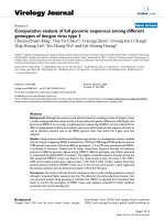
TID2008 contains 25 distortion-free test color images
(see Figure 1) and 1,700 distorted ones. Seventeen types
of distortions have been simulated including AWGN
(the first type of distortions), spatially correlated noise
(the third type of distortions), and other ones, in parti-
cular, distortions in filtered images because of residual
noise and imperfection of filters. Four levels of distor-
tions are provided adjusted so that PSNR values are

about 30, 27, 24, and 21 dB for each color image (see
[29,40] for more details).
Nowadays people use the TID2008 for some other pur-
poses than it was originally created [49,50]. Since this
image database already contains noisy and reference
images, it can be also exploited for testing image filtering
efficiency. Moreover, having noise-free images at disposal,
it is easy to add noise to them with any required variance
and, in general, any type and st atistical characteristics.
Note that all t he images, i n opposite to original Kodak
database, are of equal size that provides additional benefits
in their processing and analysis. The images are of differ-
ent content and complexities (complexity here means a
percentage of pixels that belong to image homogeneous
regions). In this sense, the images ##3 and 23 (Figure 1)
are the simplest whilst the images ##13, 14, 5, 18 are the
most complex ones. The image #25 is not from Kodak
database. It was synthesized by the authors of TID2008 to
test metric performance for artificial images. In general,
1
2 3
4
5
6 7 8 9 10
11 12 13 14 15
16 17 18 19 20
21 22
2
3
24

25
Figure 1 Noise-free test color images of TID2008 (each image has 384 rows and 512 columns, 24 bits per pixel).
Fevralev et al. EURASIP Journal on Advances in Signal Processing 2011, 2011:41
/>Page 3 of 19
no obvious differences between metric performance for
real life and artificial images have been observed in
experiments.
The PSNR values equal to 30, 27, 24, and 21 dB men-
tioned above are provided for AWGN and spatially corre-
lated noise by setting variance values s
2
equal to 65, 130,
260, and 520, respectively, for images with 8-bit represen-
tation in each color (R, G, and B) component. Noise
independence in color components has been assumed.
Spatially correlated noise has been obtained by filtering
2D AWGN by 3 × 3 mean filter with further setting a
required noise variance. After adding noise, noisy image
values have been returned into the limits 0 255, i.e., clip-
ping effects are observed in noisy images.
The case of noise variance equal to 65 (distortion level
1) is the most interesting from practical point of view
since the noise is clearly visible for most images and,
thus, it is desirable to apply filtering. The same relates
to noisy images with noise variance s
2
= 130. Mean-
while, noise variances 260 and 520 seldom met in prac-
tice. Thus, let us concentrate on more thorough
studying the cases of noisy images with s

2
= 130, 65,
and less. For all the values of noise variance smaller
than 65, images corrupted by i.i.d. and spatially corre-
lated nois e have been obtained similarly as for TID2008
images.
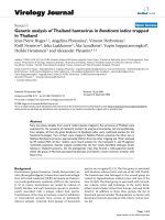
Let us illustrate some effects observed for noisy images.
Figure 2a shows the test image #16 corrupted by i.i.d.
noise with variance 65. Noise is visible in homogeneous
image regions but masked in textural regions. The same
test image corrupted by spatially correlated noise with the
same variance is presented in Figure 2b. It is obvious that
the visual quality of the latter image is worse. Noise is well
seen in practically all parts of this image. For both images,
the values of input PSNR defined as PSNR
inp
=10log
10
(255
2
/s
2
) are e qual to 30 dB. For the i mage in Figure 2a,
the metric PSNR-HVS-M [31] equals to 33.2 dB whilst for
the image in Figure 2b PSNR-HVS-M = 26.6 dB ( larger
PSNR-HVS-M relates to better visual qual ity). Thus, also
from example one can see that PSNR-HVS-M charac-
terizes image visual quality more adequately than conven-
tional PSNR.
The reason is that the metric PSNR-HVS-M accounts

for two important features of HVS. First, it exploits the
fact that sensitivity to distortions in low spatial frequen-
cies is larger than to distortions in high spatial frequen-
cies. Second, masking effect (worse ability of human
vision to notice distortions in heterogeneous and tex-
tural image areas) is taken into account.
3. Potential limits and preliminary analysis of
filter efficiency
As it has been mentioned in Section 1, there is a possi-
bility to derive lower bound output MSE (further
denoted as MSE
lb
) for denoising a grayscale image cor-
rupted by i.i.d. noise [43] under c ondition that one
also has the corresponding noise-free image. This
allows determining MSE
lb
for component-wise proces-
sing of color images in TID2008 for the first type of
distortion (i.i.d. Gaussian noise). The obtained results
for 11 color images from TID2008 (s
2
= 65) are pre-
sented in Table 1. We have selected for analysis the
most textural images (##13, 14, 5, 6, 8, 18), the sim-
plest structure test images (##10 and 23), one example
of typical (middle complexity) images (#11), and the
artificial image #25.
The analysis shows the following:
1. For a given image, the values MSE

lb
are close to
each other, this is explained by known high similar-
ity (inter-component correlation) of information
content in component R, G, and B images;
a b
Figure 2 The test image #16 corrupted by i.i.d. (a) and spatially correlated (b) noise with s
2
=65.
Fevralev et al. EURASIP Journal on Advances in Signal Processing 2011, 2011:41
/>Page 4 of 19
2. The values MSE
lb
can differ by up to 10 times
depending upon image complexity (compare MSE
lb
values for the test images ##13 and 23); this conclusion
is in good agreement with data presented in the article
[43] where it has been shown that the difference can
be even larger;
3. The larger MSE
lb
values are observed for more com-
plex-structure images, for the image #13 MSE
lb
is only
about 1.55 times smaller than s
2
= 65; thus, even
potential quality improvement because of filtering in

terms of output MSE or output PSNR (PSNR
out
)is
quite small;
4. Meanwhile, for other images improvement of PSNR
(that can be characterized by PSNR
out
-PSNR
inp
)can
be considerable, up to 11 dB for the test image #23.
For our further study, it is important to recall some
conclusions resulting from the previous analysis [40]. To
provide better visual quality of a filtered image com-
pared to the corresponding noisy one, it is necessary to
ensure that PSNR improvement because of filtering is,
at least, 3 6 dB (the smaller PSNR for noisy image, the
larger PSNR improvement should be). The latter conclu-
sion is based on the analysis of averaged mean opinion
score (MOS) [40] but it can be different for particular
images.
So, let us briefly look a t output MSE values (MSE
out
)
provided by some recently proposed filters applied com-
ponent-wise. Consider first a standard DCT-based filter
with 8 × 8 fully overlapping blocks and hard thresholding
with the threshold T =2.6s [47] where s is supposed to
be known apriori. The obtained output MSEs denoted
as MSE

DCT
are presented in Table 1. Their analysis
allows us to draw the following preliminary conclusions:
1. There is an obvious correlation between MSE
lb
and MSE
DCT
: to large r MSE
lb
corresp onds the larger
MSE
DCT
;
2. For larger MSE
lb
, the ratio MSE
DCT
/MSE
lb
is smal-
ler, i.e., the standard DCT filter provides efficiency
close to the potential limit; the same tendency has
been observed in [43] where it has been demonstrated
that the state-of-the-art filters possess efficiency close
to the reachable maximum for complex-structure
images especially if noise variance is large; for such
situations there is a very limited room for further
improvement of filter performance;
3. Considerable room for further impr ovement of fi l-
ter pe rformance exists for the simplest-structure

images (e.g., ##23 and 10, but MSE
DCT
for them is
already quite small; thus, further improvement of fil-
ter performance is not so crucial);
4. The results for artificial image #25 are similar to
those ones for typical real-life images as the image
#11.
One can argue that the standard DCT-based filter is
not the best. Because of this, for comparison purposes we
also present some results [51] for a more elaborated filter
BM3D [16] shown to be the best in [43]. For s
2
= 65 and
R component of color images, the BM3D filter produces
MSEs equal to 27.8, 28.3, 45.0, 29.4, 27.5, and 11.5 for
the images ##5, 8, 13, 14, 18, and 23, respectively. Com-
parison of these data to the corresponding data in Table
1 shows that the BM3D is slightly more efficient than the
DCT-based filter and it produces closer output MSEs to
MSE
lb
. However, the difference is not significant. It is
noted that thorough comparison of different filters is not
the main goal of thi s article . Here, it is important that
DCT-based filters perform close to currently reachable
limit.
We have also deter mined MSE
lb
for the cases s

2
=130
and 260. For a given test image, MSE
lb
for the case s
2
=
130 is about 1.7 1.8 times larger than MSE
lb
for s
2
= 65.
Similarly, MSE
lb
values for s
2
= 260 are about 1.7 1.8
times larger than the corresponding MSE
lb
values for
Table 1 Lower bound MSE and output MSE for the DCT-based filter for components of color images in TID2008.
Image index in TID2008 R component G component B component
MSE
lb
MSE
DCT
MSE
lb
MSE
DCT

MSE
lb
MSE
DCT
1 28.9 36.8 29.9 36.5 28.9 36.8
5 27.5 30.4 28.0 30.9 26.4 30.8
6 23.7 31.2 23.5 31.2 22.4 30.8
8 23.2 32.5 23.3 32.1 22.6 32.0
10 7.1 17.6 7.5 18.1 7.3 17.8
11 16.4 26.4 16.2 26.3 15.3 25.8
13 41.0 46.6 42.6 46.2 37.2 46.3
14 20.7 31.0 20.0 30.6 19.5 30.7
18 21.4 28.7 20.4 28.1 17.4 28.3
23 4.6 12.9 4.7 12.7 4.8 12.6
25 14.7 19.4 14.0 18.2 13.5 18.3
Fevralev et al. EURASIP Journal on Advances in Signal Processing 2011, 2011:41
/>Page 5 of 19
s
2
= 130. T he same ten dency has been observed [43] for
grayscale test images. The ratios MSE
DCT
/MSE
lb
for lar-
ger noise variances are even smaller than for s
2
= 65.
Thus, let us mainly concentrate on considering s
2

=65
and smaller values as more realistic and interesting in
practice. An interested reader can find some additional
data for s
2
= 130 in [51,52].
Unfortunately, the method and software [43] do not
allow determining potential limits of filtering efficiency for
vector filtering of color images. However, there are initial
results showing that MSE
lb
values in this case should be
considerab ly smaller than in the ca se of component-wise
processing [51,53]. We present results (output MSE
3DDCT
)
for the 3D DCT based vector filter [33] that uses “spectral”
DCT to decorrelate color components and then applies
2D DCT (see data in Table 2 for noise variances s
2
=65
and s
2
= 130). Let us, for example, consider MSE
3DDCT
for the test image #13. They are again quite close for R, G,
and B components and are approximately equal to 23 for
s
2
= 65. This is almost twice less th an MSE

lb
for compo-
nent-wise processing case (see data in Table 1). The values
MSE
3DDCT
occur to be smaller than the corresponding
MSE
lb
for the test images ##5 and 8 as well (compare data
in Tables 1 and 2). Only for the s implest test ima ge #23
the values MSE
3DDCT
are larger than the corresponding
MSE
lb
values although all MSE
3DDCT
are sufficiently smal-
ler than the corresponding MSE
DCT
.
Some other vector (3D) filters as C-BM3D [53] are
able to produce even smaller output MSE than
MSE
3DDCT
[54]. Besides, as it has recently been demon-
strated in [54], lower bounds for vector filtering is about
twice smaller than the corresponding MSE
lb
values if

noise is independent in color components.
One should not be surprised by the fact that MSE
3DDCT
and output MSE for some other vector filters can be
smaller t han the corresponding MSE
lb
.Thisdoesnot
mean that MSE
lb
values derived according to [43] are
incorrect.Thisonlydemonstratestwothings.First,the
use o f inter-component correlation being taken into
account by a filter allows considerable improvement of
filtering efficiency. Second, it is worth t rying to derive
lower bound MSE for multichannel filtering in the future.
Table 2 also presents the results for s
2
= 130. It is
seen that for a given image and color component, the
values of MSE
3DDCT
for s
2
= 130 are about 1.5 1.7
times larger than for s
2
= 65. Thus, the tendency
described above remains.
One should a lso keep in mind that nowadays there are
quite many blind (automatic) methods for estimation of

noise variance needed to set filter’s parameter (thresh-
old), see, e.g., [55-57] and refe rences therein. For i.i.d.
additive noise case, these methods allow estimating noise
variance or standard deviation accurately e nough even
for highly textural images as, e.g., the test image #13.
These methods can be applied if noise variance in color
components is not known in advance creating the basis
for fully automatic processing [58]. If noise in color
images has speci fic prop erties described in Section 1 and
the articles [18,39], we recommend using in blind estima-
tion of noise variance only the image fragments (blocks,
scanning windows) with local mean from 25 till 230.
4. Filter efficiency analysis for the TID2008 color
images, AWGN case
Let us start from brief description of the used quantita-
tive criteria of filtering efficiency. T he filter output
MSEs for color image components are calculated as
σ
2
k out
=
I

i=1
J

j
=1
(I
f

kij
− I
true
kij
)
2
/I
J
(1)
where
I
f
ki
j
is ijth sample of filtered kth component of a
color image in RGB representation,
I
true
ki
j
denotes true
(noise-free) value of ijth pixel of kth component, k =
1,2,3; I, J define a processed image size (384 rows and
512 columns for TID2008 color images).
Output PSNR for the considered 8-bit representation
of each color component is determined as
PSNR
k
=10log
10

(255
2
/σ
2
k out
)
(2)
Alongside with the standard PSNR, we have analyzed
the visual quality metric PSNR-HVS-M. For calculating
PSNR-HVS-M, weighted MSE
σ
2
k
H
VS
−
M
is derived first
(see details in [31]), and then
PSNR-HVS-M
k
=10log
10
(255
2
/σ
2
k
H
VS

-M
)
(3)
The source code is available at omar-
enko.info/psnrhvsm.htm. Similar to PSNR, PSNR-HVS-M
Table 2 Output MSE for the 3D DCT based filter [33] for four color images in TID2008
Component Image
Test image #13 Test image #5 Test image #8 Test image #23
s
2
=65 s
2
= 130 s
2
=65 s
2
= 130 s
2
=65 s
2
= 130 s
2
=65 s
2
= 130
R 22.0 38.9 17.3 29.1 18.2 33.2 9.0 13.8
G 22.6 40.8 17.3 29.4 17.5 33.4 8.8 13.7
B 24.6 42.1 17.5 29.2 18.8 31.3 9.5 14.6
Fevralev et al. EURASIP Journal on Advances in Signal Processing 2011, 2011:41
/>Page 6 of 19

is expressed in dB. Larger values correspond to better
visual quality. The ca ses PSNR -HVS-M > 40 dB relate to
almost perfect visual quality where noise and distortions
are practically not seen [59]. Also note that dynamic range
D of image representation should be used in (2) and (3)
instead of 255 if images are not in 8-bit representation.
Let us first consider the d ependences PSNR-HVS-M
k
(n), where n denotes index in TID2008, before and after
filtering for s
2
= 65 (see Figure 3a).
The lower group of three curves corresponds to input
(noisy) images and the upper group to t he filtered ones,
respectively. There are several important observations
that follow from the analysis of these curves:
1. Again, the curves for all color components are
very similar; this relates to both the group of input
(noisy) images and output (filtered) ones.
2. For original (noisy) images, the lowest visual qual-
ity takes place for the simplest structure images (the
smallest values of PSN R-HVS-M
k
(n) are observed
for the test images ##2, 3, 4, 15, 16, 20, and 23,
about 33 dB for all of them); this deals with the fact
that for textural images noise is considerably masked
while for simple structure images it is well seen in
homogeneous image regions.
3. For all the test images, their visual quality has

been improved; however, improvement is quite dif-
ferent, the larg est improvement is observed for sim-
ple structure images as, e.g., the test images ##3, 15,
23; the smallest improvement takes place for the
most complex s tructure test images as, e.g., the t est
images ##5, 13, and 14.
It is noted that different efficiencies of image filtering
result from the test image properties. For example, the
test image #13 is, obviously, more compl ex than the test
images #3 and #23. T he problem of efficient filtering of
textural imag es is typical and crucial not only for DCT-
based filters but also for almost all the filters as well.
Generally speaking, this is one of the most complicated
problems in image filtering (see also data in Table 1).
Here, we would li ke to draw readers’ attention to
recently obtained results [59]. Visibility of distortions
has been analyzed for images compressed in a lossy
man ner. It has been shown that for PSNR-HVS-M > 40
dB or MSSIM > 0.99 the distortions are practical ly non-
noticeable. We have checked this for color noisy and fil-
tered images as well as for images with watermarks. It
has been established that the aforementioned property
holds.
Keeping this in mind, it is possible to state that f or
AWGN with s
2
= 65 noise is clearly visible in original
images (the values of PSNR-HVS-M
k
(n)arewithinthe

limits 33 36 dB, see the lower group of curves in Figure 3).
In processed images, residual noise and distortions intro-
duced by filtering are less noticeable but anyway visible.
We have also considered several values of AWGN
noise variance smaller than 65 (the corresponding noisy
images have been generated using the reference images
in TID2008). Consider the most interesting case of s
2
=
25. It is noted that for s
2
=25PSNR
inp
is equal to 34.1
dB for all noisy images. The results are presented in Fig-
ure 3b. The lower group of three curves relates to the
noisy images and the upper group corresponds to the
filtered ones. The main conclusions drawn from the
analysis of these curves are the same as conclusions 1-3
given above. The difference consists in the following.
The smallest values of PSNR-HVS-M
k
(n) observed for
the noisy test images ##2, 3, 4, 15, 16, 20, and 23 are
within the limits 37.5 38 dB, i.e., considerably larger
n
(), dB
k
PSNR HVS M n
n

()
,
d
B
k
PSNR HVS M n
a B
Figure 3 PSNR-HVS-M
k
(n) before (thin lines) and after filtering for s
2
= 65 (a) and 25 (b), AWGN.
Fevralev et al. EURASIP Journal on Advances in Signal Processing 2011, 2011:41
/>Page 7 of 19
than for the case of s
2
= 65. For the most complex
structure images as, e.g., the test images ##5, 8, 13, and
14, the values of PSNR-HVS-M
k
(n) are larger than 40
dB even for noisy (not filtered) images and there is no
need to process them to improve visual quality.
For almost all the filtered test images, the values of
PSNR-HVS-M
k
( n) are larger than 40 dB. This means
that processed images are practically indistinguishable
from the corresponding reference ones. Moreover, if
more sophisticated filtering methods than component-

wise DCT-based denoising are applied, then it is possi-
ble to provide almost “ideal” visual quality of processed
images (PSNR-HVS-M
k
> 40 dB) for values of noise var-
iance larger than 25. As examples, let us give da ta for
two images from TID2008: one of the simplest ones
(#3) and one of the most complex (#13). If the 3D DCT
filter [33] is applied to the test image #3 corrupted by
AWGN with s
2
= 35, the values of PSNR-HVS-M
k
are
equal to 41.84, 41.94, and 41 .47 dB for R, G, and B
components, respectively. Similarly, for the image #13
we have 42.66, 42.00, and 41.1 dB (all over 40 dB).
Thus, the upper limit of AWGN variance for which fil-
tered images are indistinguishable from reference ones
is even higher if efficient 3D filters are employed.
Our studies have also shown that if s
2
≤ 10 15, noise
is practically (with large probability) invisible in original
images. This means t hat there is no reason to apply fil-
tering if AWGN noise has variance s
2
≤ 10 15.
In terms of conventional PSNR
k

, the smallest values
for s
2
= 25 are observed for the components o f the
complex-structure test image #13 (about 35 dB) while
for the simplest test images (##3, 7, 20, 23, and 25) the
values of PSNR
k
reach 40 dB. Therefore, in terms of
PSNR
k
, component-wise DCT-based filtering is still effi-
cient. More complicated filters [33,53] are able to pro-
vide even larger increase of PSNR after denoising.
A practical question is then can anyone predict effi-
ciency of filtering or is it reasonable to pe rform filtering
for a given image? For this purpose, one has to be sure
that noise is i.i.d. Second, one has to be confident that
noise variance is smaller than 15 (then no filtering can
be performed), if component-wise DCT-based filtering
is to be applied and smaller t han 35 if 3D DCT-based
denoising has to be carried out. Earlier, we mentioned
the methods for blind evaluation of noise variance
which are accurate enough. Thus, it could be also nice
to have a parameter allowing to establish is noise i.i.d.
or not.
One such parameter has been proposed in [36]. The
methodology of its determination i s the following. For
each block with its left upper corner characterized by
indices l and m, two local estimates of noise variance

are calculated in spatial domain as
σ
2
klm
=
l
+7

i=l
m+7

j
=m
(I
kij
−
¯
I
klm
)
2
/63;
¯
I
klm
=
l
+7

i=l

m+7

j
=m
I
kij
/6
4
(4)
and in DCT domain as
(σ
sp
klm
)
2
= (1.483med(



D
lm
qs



))
2
,
(5)
where

D
lm
q
s
, q = 0, , 7, s = 0, , 7, except q = s =
0
are DCT coefficients of lmth block of kth component of
a given color image. Then, for each block the following
ratio is calculated
R
klm
= σ
klm
/σ
sp
klm
. The histogram of
theseratiosisformedanditsmode

r
k
(
n
)
is determined
by the method given in [60]. The distribution of R
klm
for all k and almost all images has quasi -Gaussian com-
ponent with a maximum coordinate close to unity (for i.
i.d. noise) and a right-hand heavy tail where the ratios

relating to this tail are obtained in heterogeneous image
blocks.
Let us analyze the behavior of the estimates

r
k
(
n
)
.
The dependences of

r
k
(
n
)
on n for all color components
are given in Figure 4 as the curves of the correspond ing
color (for s
2
= 65 and 25). As seen, these dependences
are very similar. Almo st equal val ues of

r
k
(
n
)
are

observed for R, G, and B components of a given test
color image an d a fixed noise variance. Some sufficient
differences in the values

r
k
(
n
)
, k =1,2,
3
are only seen
for the test image #20. The reason is in considerable
clipping effects observed for this test image. The values

r
k
(
n
)
for larger noise variance are slightly smaller (com-
pare these values for the same images in Figure 4a, b).
The most important observation is that the largest
values

r
k
(
n
)

take place f or the most textural images as
the test images ##5, 8, 13, 18. For other test images, the
values

r
k
(
n
)
are quite close to unity. Thus, the para-
meter

r
k
(
n
)
seems to be “correlated” with image com-
plexity and filtering efficiency. To check this
assumption, let us determine Spearman rank correlation
factor [61] (note that here rank correlation is used to
avoid fitting problems). First, we have calculated Spear-
man rank correlation R
kSp
for data arrays

r
k
(
n

)
(Figure
4a) and PSNR
k
( n)atfilteroutputs,n = 1, ,25. For all
the color components, the values R
kSp
are in the range
-0.9 0.8. The fact that the values of R
kSp
are negative
means that reduction of

r
k
(
n
)
relates to an increase of
PSNR
k
(n). The fact that absolute values of R
kSp
are quite
large (close to unity) shows that there exists consider-
able and strict correlation between

r
k
(

n
)
and PSNR
k
(n).
We have also calculated R
kSp
for data arrays

r
k
(
n
)
(Figure 4b) and PSNR
k
(n) at filter outputs, n = 1, 25 for
noisevarianceequalto25.ThevaluesR
kSp
fall to the
same range. Thus, larger increase of PSNR can, most
probably, be provided if

r
k
(
n
)
is small.
Fevralev et al. EURASIP Journal on Advances in Signal Processing 2011, 2011:41

/>Page 8 of 19
Besides, if noise is i.i.d., then a considerable deviation
of

r
k
(
n
)
from 1.0 (e.g.,

r
k
(
n
)
is larger than 1.08) shows
that an image to be filtered is quite complex (is textural
and/or contains many fine details). In turn, it also
means that for this image it is difficult to expect effi-
cientfilteringinthesenseofconsiderableincreaseof
PSNR-HVS-M.
Sufficient correlation also exists between

r
k
(
n
)
(Figure

4) and PSNR-HVS-M
k
(n ) before filtering (lower groups
of curves in Fig ure 3). The Spearman rank correlation
factors for these arrays R
kSp
are within the limits
0.8 0.9. Positive values mean that if

r
k
(
n
)
is rather
small, then the corresponding PSNR-HVS-M
k
(n)is
rather small too. Then, noise in a given image is not
considerably masked. Therefore, the parameter

r
k
(
n
)
tha t can be determined for an image in advance (befor e
filtering) can serve for characterizing image complexity
and noise masking effects as well as predicting efficiency
of filtering. Further analysis results and conclusions are

presented in the following section.
Here, we would like to give more insights on visual
quality of noisy and filtered images. For this purpose, let
us recall how the metric PSNR-HVS-M (3) is calculated
[31]. The first step is to determine s
2
HVS-M
. This p ara-
meter is an average of local MSEs s
2
HVS-M lm
:
σ
2
HVS - M
=
I−7

l
=1
J−1

m=1
σ
2
HVS - M lm
/((I − 7)(J − 7)
)
.LocalMSEs
s

2
HVS-M lm
are calculated in 8 × 8 blocks with left upper
corner defined by indices l and m and they are deter-
mined in DCT domain with taking into account contrast
sensitivity f unction and masking [31] . Local MSEs
s
2
HVS-M lm
can be smaller or larger than noise variance.
The inequality s
2
HVS-M lm
>s
2
usually holds if noise is
spatially correlated (or realization of i.i.d. noise in a
given block exhibits such quasi-correlation) and/or there
is no masking for a given block (this mostly happens for
homogeneous image blocks).
Consider as one example the G component of the test
image #14 corrupted by i.i.d. noise with variance 25
(shown in Figure 5a). Noise can be hardly noticed in
homogeneous image regions as the gum boat surface. In
other places, as water surface noise is practically not
seen because of masking effects. These observati ons are
confirmed by the map of s
2
HVS-M lm
for noisy (original)

image presented in Figure 5b (further denoted as s
2
HVS-
Morlm
, brighter pixels correspond to blocks with larger
s
2
HVS-M or lm
). The histogram of s
2
HVS-M or lm
is shown
in Figure 6a. It is seen that there are values of s
2
HVS-M
or lm
larger than 25 but this happens quite seldom and
mostly in homogeneous i mage regions (analyze the
noisy image in Figure 5a and the map of s
2
HVS-M or lm
in Figure 5b jointly).
Consider now the estimates s
2
HVS-M or lm
for the
image processe d by the DCT-based filter (further
denoted as s
2
HVS-M fi lm

). The corresponding map is
presented in Figure 5c (brighter pixels correspond to
blocks with larger s
2
HVS-M fi lm
) and the histogram is
giveninFigure6b.Analysisofthehistogramshows
that, on the average, the values of s
2
HVS-M fi lm
are
smaller than s
2
HVS-M or lm
although there are s
2
HVS-M fi
lm
larger than 25. This takes place in textural regions
and in edge/detail neighborhoods (analyze the noisy
image in Figure 5a and the map of s
2
HVS-M fi lm
in Fig-
ure 5c jointly).
Finally, we have obtained the map of the ratio s
2
HVS-M
fi lm
/s

2
HVS-M or lm
(presented in binary form in Figure
5d)andthehistogramofthisratio(seeFigure6c).His-
togram analysis demonstrates that mostly the ratios are
n
()

k
rn
n
()

k
rn
a b
Figure 4 Dependences

r
k
(
n
)
for components of color images for s
2
= 65 (a) and 25 (b).
Fevralev et al. EURASIP Journal on Advances in Signal Processing 2011, 2011:41
/>Page 9 of 19
smaller than unity, i.e., local improvement of visual
qualityisprovidedbyfiltering.Thismostlyoccursin

homogeneous image regions. However, there are also
local degradations of visual quality when distortions
introduced because of filtering are larger than positive
effect of noise removal. The places where such degrada-
tions are the most considerable are shown by white in
the binary map in Figure 5d. Joint analysis of the noisy
imageinFigure5aandthebinarymapinFigure5d
allows concluding that the largest local degradations of
a
b
c d
Figure 5 Green component of noisy image # 14 (a), the map of s
2
HVS-M lm
for noisy image (b), the map of s
2
HVS-M lm
for filtered
image (c), the ratio map in binary form, black if s
2
HVS-M fi lm
/s
2
HVS-Morlm
< 1.5 and white otherwise (d).
0 10 20 30 40 50 60
0
0.5
1
1.5

2
2.5
3
3.5
x 10
4
a
0 10 20 30 40 50 60
0
0.5
1
1.5
2
2.5
3
3.5
x 10
4
b
0 0. 5 1 1.5 2 2.5 3
0
2000
4000
6000
8000
10000
12000
c
Figure 6 Histograms of s
2

HVS-Morlm
for noisy image (a), s
2
HVS-M fi lm
for filtered image (b), and s
2
HVS-M fi lm
/s
2
HVS-Morlm
(c).
Fevralev et al. EURASIP Journal on Advances in Signal Processing 2011, 2011:41
/>Page 10 of 19
visual quality take place in heterogeneous image regions
(edge/detail neighborhoods, high contrast textures).
Let us see what improvement of image visual quality
can be produced by the BM3D filter [16] applied compo-
nent-wise. Figure 7a shows the histogram of the ratio
s
2
HVS-M fi lm
/s
2
HVS-M or lm
for this filter. It is similar to
the histogram in Figure 6c. Figure 7b demonstrates the
ratio binary map. Its comparison to the binary map in
Figure 5d shows that the number of white p ixels (for
which s
2

HVS-M fi lm
/s
2
HVS-M or lm
> 1.5 and, thus , BM3D
filtering introduces considerable distortions) is smaller
than for the conventional DCT-based filter. Note that the
values of PSNR-HVS-M
k
(14) for the BM3D filter are only
by 0.3 0.4 dB larger than for the DCT-based filter. Thus,
visual quality im provement is not large w hile complexity
of BM3D is sufficiently greater.
Consider now another, simpler structure, test image #3
corrupted by AWGN with larger noise variance equal to
65. It’s noisy green component is represented in Figure
8a. The noise is well seen, especially in homoge neous
image regions. The map of s
2
HVS-M or lm
for this noisy
image is shown in Figure 8b (brighter pixels correspond
to blocks with larger s
2
HVS-M or lm
). Masking effect is
well observed for edge neighborhoods (dark pixels that
appear on them show that the values of s
2
HVS-M or lm

are
considerably smaller than in other places). The corre-
sponding histogram of s
2
HVS-M or lm
isgiveninFigure
9a. It is seen that there are values of s
2
HVS-M or lm
larger
than 65 although this happens very seldom, mostly in
homogeneous image regions (analyze the noisy image in
Figure 8a and the map in Figure 8b jointly).
The estimates s
2
HVS-M fi lm
for the image processed by
the DCT-based filter component-wise are presented in
Figure 8c, the corresponding histogram is shown in Figure
9b. The histogram analysis clear ly demonstrates that, on
the average, the values of s
2
HVS-M fi lm
have become
considerably smaller than s
2
HVS-M or lm
although there is
still a small percentage of s
2

HVS-M fi lm
larger than 65.
Such blocks occur in neighborhoo ds of high contrast
edges and fine details (from the joint analysis of the noisy
imageinFigure8aandthemapinFigure8c).The
obtained map of the ratio s
2
HVS-M fi lm
/s
2
HVS-M or lm
is
presentedinbinaryforminFigure8d,thehistogramof
this ratio is given as well (Figure 9c). The analysis of the
histogram shows that for a large percentage of pixels
(blocks) the ratios are smaller than unity. This means that
a local improvement of visual quality is provided due to
the filtering. This improvement is sufficient since there are
many values of the ratio smaller than 0.5. As it can be
expected, sufficient improvement of loc al visual quality
takes place mainly in homogeneous image regions.
However, even for the considered simple structure test
image, there exist local degradations of visual quality as
well. The map in Figure 8d sh ows that distortions intro-
duced because of filtering are large fo r sharp edge and
detail neighborhoods (shown as white in the binary map
in Figure 8d). This conclusion once more stresses the
known drawback of the DCT-based filter to introduce
distortions in places of sharp transitions in i mages
[25,62]. It means that if visual quality of filtered images is

of prime importance, the attention in filter design should
be paid to the preservation of e dges and fine details in
the first order. In this sense, non-local filtering methods
are able to provide certain benefits w.r.t. DCT-based fil-
tering. It is noted that attention of observers to edge/
detail neighborhoods has been stated in several articles
and used in design of visual quality metrics [28,30,63].
5. Filter efficiency analysis: spatially correlated
noise case
Having studied the i.i.d. noise case, let us consider now
filtering of images corr upted by spatially correlated noise.
0 0.5 1 1.5 2 2.5 3
0
2000
4000
6000
8000
10000
12000
a
b
Figure 7 The histogram of the ratio s
2
HVS-M fi lm
/s
2
HVS-Morlm
(a) and its binary map (b) for the BM3D filter.
Fevralev et al. EURASIP Journal on Advances in Signal Processing 2011, 2011:41
/>Page 11 of 19

First, there are less filters designed and tested for spatially
correlated noise removal (see [35,36,64-67] and refer-
ences therein). Second, under the assumption of spatially
correlated noise presented in images, several questions
arise immediately: what is a model for spatially correla-
tion noise, w hat aprioriinformation on characteristics
(statistical, spatial spectrum) is available, are 2D spatial
spectrum or correlation function the same for all parts of
a processed image (does an assumption on stationarity of
noise or invariance of its characteristics hold)?
These are questions of additional studies and answers
to them depend on practical application at hand. To
a
B
c d
Figure 8 Green component of noisy image # 14 (a), the map of s
2
HVS-M lm
for noisy image (b), the map of s
2
HVS-M lm
for filtered
image (c), the ratio map in binary form, black if s
2
HVS-M fi lm
/s
2
HVS-M or lm
< 1.5 and white otherwise (d).
0 10 20 30 40 50 60 70 80 90 100

0
1000
2000
3000
4000
5000
6000
7000
8000
9000
10000
a
0 10 20 30 40 50 60 70 80 90 100
0
0.5
1
1.5
2
2.5
3
x 10
4
b
0 0.5 1 1.5 2 2.5 3
0
0.5
1
1.5
2
2.5

3
x 10
4
c
Figure 9 Histograms of s
2
HVS-M or lm
for noisy image (a), s
2
HVS-M fi lm
for filtered image (b), and s
2
HVS-M fi lm
/s
2
HVS-M or lm
(c).
Fevralev et al. EURASIP Journal on Advances in Signal Processing 2011, 2011:41
/>Page 12 of 19
simplify the situation, let us assume that spatially corre-
lated noise is pure additive and stationary in the sense
that its 2D spatial spectrum is the same for all parts of
images to be processed. Howeve r, even in this case
there is a wide variety of possible variants of 2D sp ectra
of spatially correlated noise. To partly alleviate this
uncertainty, we, first, assume that noise spectrum (in
DCT domain for 8 × 8 blocks) is known in advance or
estimated in a blind manner with appropriate accuracy
[64]. Second, in our simulations we consider two models
of spatially correlated noise that differ from each other

by 2D spatial DCT spectra in terms of their shape or,
equ ivalently, main lobe width of 2D spati al autocorrela-
tion function (ACF). In other words, we carry out brief
analysis how the main properties of spatially correlated
noise ACF influence original image visual quality and
efficiency of DCT-based filtering.
For spatially correlated noise case, thresholds for the
corresponding modificationoftheDCT-basedfilter
(MDCT-based filter) should be frequency dependent as
T(n, m)=2.6σ

W
norm
(n, m)
where W
norm
(n, m)isthe
normalized DCT spectrum for the block size used, n
and m are frequency indices. It is noted that the DC
coefficients in blocks are not thresholded (changed)
while carrying out filtering [35,37].
It is noted that in the case of additive spatially corre-
lated noise, its spatial correlation should be taken into
account. The standard DCT-based filter with fixed (fre-
quency independent) threshold is not efficient for
removal of spatially correlated noise. This has clearly
been demonstrated in terms of output PSNR [35,37]
and in terms of the metric PSNR-HVS-M [35,52]. The
difference in output PSNR for the standard and MDCT
filters can be from 1 to 4 dB [35,37,52]. T he increase is

the smallest for complex-structure images as the test
image #13 (about 1.5 dB) but it can reach 4 dB for sim-
ple-structureimagesasthetestimage#3fornoisevar-
iance equal to 65. However, the provided values of
PSNR
k
( n) for the MDCT-based filter are smaller than
for i.i.d. noise case for each of the analy zed test images
[62]. This shows that removal of spatially correlated
noise is a more difficult task than AWGN filtering.
The difference of the metric PSNR-HVS-M values for
the considered standard (with frequency independent
threshold) and MDCT filters is sufficient (up to 3 dB).
Dependences PSNR-HVS-M
k
(n) for components of
color images before filtering (the lower group if three
curves) and after image denoising by the standard DCT-
based filter (the upper group of three curves, s
2
=65)
are presented in Figure 10a. It is seen that the presence
of spatially correlated noise leads to a larger degradation
of image visual quality than that with the presence of
AWGN under condition that noise variance is the same
(com pare the lower groups of curves in Figures 10a and
3a). As can be seen also, the standard DCT-based filter-
ing produces improvement of visual quality of processed
imagesforallthetestimages.TheincreaseofPSNR-
HVS-M after filtering ranges from 0.7 dB for the most

textural images to 2.5 dB for the simplest test images.
Dependences PSNR-HVS-M
k
(n ) for the output of the
MDCT filter are r epresented in Figure 10b. Comparison
to the upper group of curves in Figure 10a demonstrates
that the MDCT filter produces considerably larger
improvement of output image visual quality. However,
the worst results (the smallest values of PSNR-HVS-M
k
(n) are observed for the most textural (complex-struc-
ture) test images ##1, 5, 13, 14, and 18.
Thus, it is reasonable for applying the MDCT-based
filtering with frequency-dependent thresholding adapted
to DCT spectrum of spatially correlated noise. Because
of this, below we consider only this filter. The main
attention is paid to the values of noise variance smaller
than 65, since, as it is seen for plots in Figure 10, noise
is clearly seen in original and filtered images for the
case of s
2
=65(thevaluesofPSNR-HVS-Maresuffi-
ciently smaller than 40 dB).
As it was mentioned above, it is worth analyzing spa-
tially correlated noise with different spatial spectra.
Images in TID2008 are corrupted by spatially correlated
noise obtained by applying the 3 × 3 mean filter to 2D
AWGN.Inthissection,wecontinuetosimulatespa-
tially correlated noise in this manner but with variance
smaller than 65 (this case is treated as considera ble cor-

relation noise–CCN). Besides, we simulate middle corre-
lation noise (MCN) by applying to 2D AWGN the
linear 3 × 3 scanning window FIR filter with weights
⎡
⎣
1/4 1/2 1/4
1/211/2
1/4 1/2 1/4
⎤
⎦
Such filter is characterized by wider spectrum and,
respectively, narrower main lobe of 2D ACF. By simulat-
ing large size 2D arrays of pure spatially correlated noise
in this way, it is possible to estimate W
norm
(n, m)used
in MDCT-based filter quite accurately. The 8 × 8
matrices of (W
norm
(n, m))
0.5
for both variants of spa-
tially correlated noise are given below. It is seen that the
values of (W
norm
( n, m))
0.5
for low frequencies (upper
left corner) and high frequencies (lower right corner)
differ a lot, especially for CCN case. Matrix elements

symmetrical with respect to the main diagonal are prac-
tically equal to each other. Difference of their values is
explained by a finite size of 2D arrays of simulated noise
used for spatial spectrum estimation.
Since spatially correlated noise with s
2
=65isclearly
visible in original and filtered images, let us consider
Fevralev et al. EURASIP Journal on Advances in Signal Processing 2011, 2011:41
/>Page 13 of 19
sufficiently smaller values of noise variance. Figure 11
shows the dependences of PSNR-HVS-M
k
(n), dB for
components of color images for noise vari ance equal to
nine for CCN and MCN. As previously described, lower
groups of curves correspond to the original (noisy)
images while the upper groups relate to the filtered
images.
The curves’ behavior is very similar. The only differ-
ence is that, for a given test image, its visual quality is
slightly better for MCN case than for CCN both before
and after filtering. As it can be expected, visual quality
improves because of filtering although this improvement
is small for complex-structure images and it can reach
up to 4 dB for simple-structure images. For both CCN
and MCN, noise is visible in all original the test images
since PSNR-HVS-M
k
( n) < 40 dB. However, even after

filtering residual noise and introduced distortions
remain visible in most output images. This means that
the task of image filtering with the purpose of their
enhancement (visual quality improvement) is crucial for
spatially correlated noise case even for rather small
values of noise variance.
Consider now smaller values of noise variance, equal
to 6. The obtained dependences are represented in Fig-
ure 12. Analysis of these dependences shows the follow-
ing. Spatially correlated noise is still visible in most
original noisy images, especially simple structure ones
(visu al inspection has shown that noise can be visible in
n
()
,
d
B
k
PSNR HVS M n
n
(), dB
k
PSNR HVS M n
a b
Figure 10 Dependences PSNR-HVS-M
k
(n), dB for components of color images (spatially correlated noise, s
2
= 65) before (thin lines)
and after filtering by the standard DCT-based filter (a) and by its modification with frequency dependent thresholds (b).

n
()
,
d
B
k
PSNR HVS M n
n
(), dB
k
PSNR HVS M n
a b
Figure 11 Dependences PSNR-HVS-M
k
(n), dB for c omponents of color images (s
2
= 9) before (thin lines) and after filtering by the
MDCT-based filter for CCN (a) and MCN (b).
Fevralev et al. EURASIP Journal on Advances in Signal Processing 2011, 2011:41
/>Page 14 of 19
homogeneous regions of such images). However, accord-
ing to the rule PSNR-HVS-M
k
(n) > 40 dB, residual noise
and introduced distortions become practically invisible
after filtering.
One can argue that we use DCT-based filters and
DCT-based visual quality metr ic PSNR-HVS-M in our
analysis and it is not fair enough. To avoid such possible
criticism, we have also analyzed the wavelet-based

metric MSSIM [27]. Recall that this metric is within the
limits from 0 (very bad quality) to 1 (perfect quality). If
MSSIM is larger than 0.985 0.99, distortion s are practi-
cally not seen.
The dependences of MSSIM
k
(n)forMCNwiths
2
=9
are shown in Figure 13a. Their analysis allows drawing
the same conclusions as for dependences PSNR-HVS-M
k
(n) in Figure 11b. For none original test image, its visual
quality is perfect (all MSSIM values are smaller than
0.99). For almost all the test images, residual noise and
distortions are visible after filtering. Thus, the metric
MSSIM indicates the same as PSNR-HVS-M does.
Consider now the behav ior of the parameter

r
k
(
n
)
for
a spatially correlated noise. Dependences for a particular
case of CCN with s
2
= 65 are represented in Figure
13b. These dependences for color components are very

similar. It is noted that, in contrast to AWGN case (see
Figure 4), the values

r
k
(
n
)
are about 1.55 for a lmost all
test images (the values

r
k
(
n
)
are a little bit smaller for
the MCN case). It is noted that for s
2
=6,thevalues

r
k
(
n
)
are in the limits 1.24. 1.93 for CCN and
1.15 1.96 for MCN. In any case, the main observation
is that for spatially correlated noise, the values


r
k
(
n
)
are
considerably larger than unity.
Joint analysis of

r
k
(
n
)
in Figures 4 and 13 indicates
that its rather small values, e.g., not excee ding 1.05 are
observed for simple-structure images corrupted by noise
close to i.i.d. Then, it is reasonable to expect high effi-
ciency of denoising by the standard DCT filter. In con-
trast, i.e., when

r
k
(
n
)
exceeds 1.05 1.1, the situation is
not so clear and it is difficult to distinguish complex-
structure images corrupted by i.i.d. noise and images
corrupted by spatially correlated noise. Then, it is worth

estimating spatial spectrum of the noise. This can be
performed automatically by the methods given i n
[35,64]. More details on how to use such blind estimates
in filtering can be found in the literature [35].
Thus, the image filtering can fully be blind (auto-
matic). The first stage is to obtain

r
k
(
n
)
and to compare
it to the threshold (e.g., 1.08). Then, noise variance can
be estimated if it is a priori unknown. After this, noise
spatial correlation (spectrum) characteristics are to be
determined if needed (if

r
k
(
n
)
exceeds the threshold).
Finally, the corr esponding DCT-based filtering is to be
applied with taking into account available or obtained
data on noise variance and spatial correlation character-
istics. The automatic procedure is described roughly and
needs more thorough analysis in the future.
Let us give one example for illustrating an efficiency of

the modified DCT filter. The noise-free test image #7
from TID 2008 which is a typical representative of mid-
dle complexity color images is shown in Figure 14a. It’s
noisy version (s
2
= 65, spatially correlated noise, CCN) is
giveninFigure14b.Noisehasanappearancetypicalfor
digital cameras of bad quality or operating in bad illumi-
nation conditions. The noise is well seen in homoge-
neous regions and its influence can be noticed in textural
regions. The output of the MDCT-based filter adapted to
spatial spectrum of noise (Figure 15a) is presented in Fig-
ure 14c. The noise is suppressed considerably although
n
()
,
d
B
k
PSNR HVS M n
n
()
,
d
B
k
PSNR HVS M n
a B
Figure 12 Dependences PSNR-HVS-M
k

(n), dB for c omponents of color images (s
2
= 6) before (thin lines) and after filtering by the
MDCT-based filter for CCN (a) and MCN (b).
Fevralev et al. EURASIP Journal on Advances in Signal Processing 2011, 2011:41
/>Page 15 of 19
n
(), dB
k
MSSIM n
n
()

k
rn
a b
Figure 13 MSSIM
k
(n) for MCN with s
2
= 9 before (thin lines) and after filtering (a) and

r
k
(
n
)
for CCN with s
2
=65.

a
b
c
d
Figure 14 The test color image #7: noise-free (a), noisy (b) and filtered by the component-wise (c) and 3-D MDCT (d).
Fevralev et al. EURASIP Journal on Advances in Signal Processing 2011, 2011:41
/>Page 16 of 19
residual noise is visually seen compared to the image in
Figure 14a. Useful information (edges, textures, details) is
preserved well enough although there are some artifacts
in the neighborhoods of sharp edges which are notice-
able. This is in agreement with the value of PSNR-HVS-
M approximately equal to 30.7 dB for all the color com-
ponents (see data for the test image #7 in Figure 10b).
We have also modified 3D DCT filter to be able to
remove a spatially correlated noise. Modification is as
follows. Decorrelation of color components is carried
out first. Then, MDCT-based filter adapted to known
2D DCT spectrum of the noise is applied to the
obtained components. Then, inverse 3-element DCT is
performed. For the image filtered in this way, PSNR-
HVS-M has been determined. It is equal to 32.07, 32.36,
and 32.23 dB for R, G, and B components, respectively.
As seen, these values are, on the average, by 1.5 dB lar-
ger than for MDCT-based filter applied component-
wise. The obtained output image is represented in Fig-
ure 14d. Comparison of images in Figure 14c, d shows
that the latter one has better visual quality. This one
demonstra tes more the benefits of vector (3D) proces-
sing of color images.

Concerning practical application of the obtained
results, it is worth mentioning the following.
First, the methods of blind evaluation of noise var-
iance and spatial spectrum [56,57,60,64] have not been
intensively tested for small values of noise variance (of
the order 5 20 for images with 8-bit representation). It
has been shown experimentally that the accurate estima-
tion of noise characteristics for less intensive noise is a
more complicated task than that for an intensive noise
[44,60]. Thus, such analysis should be done in the future
and, possibly, a design of new, more efficient, blind
methods will be needed.
Second, the results presented above rely on the simpli-
fied model of noise (pure additive). It is desirable to
study what happens if this assumption is used in proces-
sing real-life data or to design modified methods able to
take into account peculiarities of more realistic noise
models [68].
Third, it is worth thinking how PSNR-HVS-M or
MSSIM can be estimated without having a reference
image. Such studies have already been done for the
metric SSIM [69].
Fourth, although our studies deal with images with 8-
bit representation, the sa me conclusions are valuable for
images with wider dynamic ranges, i.e., hyperspectral
data [4]. In a more general form, PSNR-HVS-M is
defined as
PSNR-HVS-M
k
=10log

10
(D
2
/
2
k
H
VS
-M
)
where D defines dynamic range of data representation.
Then, if, e.g., PSNR-HVS-M
k
> 40 dB, then it is possible
to suppose that a noise is invisible for a visualized kth
component (subband) image of hyperspectral data. The
simula tion data provided above allow predicti ng when it
is possible to expect considerable improvement of image
quality due to a noise removal and when it is possible
to skip filtering stage.
6. Conclusions
We have extensively tested filtering efficiency of DCT-
based filters f or color images of the database TID2008
2.69 2.37 2.04 1.51 0.93 0.51 0.59 0.81
2.39 2.09 1.80 1.35 0.85 0.45 0.52 0.75
2.04 1.80 1.53 1.14 0.72 0.38 0.43 0.62
1.52 1.35 1.15 0.85 0.53 0.29 0.33 0.48
0.93 0.85 0.70 0.53 0.33 0.18 0.20 0.29
0.51 0.45 0.38 0.29 0.18 0.10 0.11 0.16
0.58 0.52 0.44 0.33 0.21 0.11 0.12 0.18

0.84 0.75 0.63 0.48 0.29 0.16 0.18 0.26
a
2.40 2.25 1.95 1.61 1.18 0.76 0.40 0.16
2.19 1.99 1.80 1.47 1.06 0.70 0.37 0.15
1.99 1.80 1.60 1.31 0.96 0.63 0.32 0.13
1.60 1.46 1.31 1.06 0.79 0.51 0.27 0.11
1.17 1.09 0.98 0.78 0.58 0.38 0.19 0.08
0.77 0.70 0.61 0.51 0.38 0.25 0.13 0.05
0.41 0.37 0.33 0.27 0.20 0.13 0.07 0.03
0.16 0.15 0.13 0.10 0.08 0.05 0.03 0.01
b
Figure 15 Matrices of (W
norm
(n, m))
0.5
for CCN (a) and MCN (b).
Fevralev et al. EURASIP Journal on Advances in Signal Processing 2011, 2011:41
/>Page 17 of 19
and additional set of noisy images obtained using refer-
ence images of this database. The images were cor-
rupted by AWGN and spatially correlated noise with a
wide set o f variance values. As it can be expected, filter-
ing efficiency considerably depends on image complexity
and noise variance. For rather simple images corrupted
by AWGN with rather large variance, filtering efficiency
is the highest according to the standard metric PSNR
and the metric PSNR-HVS-M suited for characterizing
visual quality. In cases of spatially correlated noise, high
complexity of images and small values of noise variance,
sufficient improvement of image quality due to filteri ng

is problematic. It is shown that if AWGN variance is
less than 20, noise is practically not seen. To be invisible
in original images, spatially correlated noise should have
about 3 4 times smaller variance. Residual noise and
distortions because of filtering can become invisible
after denoising if noise variance in original image is
small enough and efficient filtering, e.g., vector or 3D
filtering, is applied. In the future, it is worth paying
more attention to efficiency analysis and performance
improvement just for 3D filters.
7. Competing interests
The authors declare that they have no competing
interests.
Author details
1
National Aerospace University, 61070, Kharkov, Ukraine
2
Tampere University
of Technology, FIN 33101, Tampere, Finland
Received: 2 June 2011 Accepted: 15 August 2011
Published: 15 August 2011
References
1. Single-Sensor Imaging, Methods and Applications for Digital Cameras
(Image Processing Series). ed. by R. Lukac. (CRC Press, 2009), p. 566
2. A Theuwissen, Course on Camera System. Lecture Notes (CEU-Europe,
2005), pp. 2–5
3. J Xiuping, JA Richards, Remote Sensing Digital Image Analysis, 4th edn.
(Springer, Berlin, 2006), p. 439
4. Hyperspectral Data Exploitation: Theory and Applications, ed. by Chein-I
Chang (Wiley-Interscience, 2007)

5. S Kiranyaz, S Uhlmann, M Gabbouj, Dominant Color Extraction Based on
Dynamic Clustering by Multi-dimensional Particle Swarm Optimization. in
Proceedings of the Seventh International Workshop on Content-Based
Multimedia Indexing, CBMI 2009, 181–188 (3-5 June 2009)
6. B Smolka, KN Plataniotis, AN Venetsanopoulos, Nonlinear techniques for
color image processing. Chapter 12 in Nonlinear Signal and Image
Processing: Theory, Methods, and Applications. Electrical Engineering & Applied
Signal Processing Series, ed. by Barner K, Arce G (CRC Press, 2003), p. 560
7. G Yu, T Vladimirova, MN Sweeting, Image compression systems on board
satellites. Acta Astronautica, 64, 988–1005 (2009). doi:10.1016/j.
actaastro.2008.12.006
8. M Elad, Sparse and Redundant Representations. From Theory to Applications
in Signal and Image Processing, (Springer Science+Business Media, LLC,
2010), p. 376
9. S Morillas, S Schulte, T Melange, E Kerre, V Gregori, A soft-switching
approach to improve visual quality of colour image smoothing filters. in
Proceedings of ACIVS, Springer Series on LNCS. 4678, 254–261 (2007)
10. J Astola, P Kuosmanen, Fundamentals of Nonlinear Digital Filtering (CRC
Press LLC, Boca Raton, 1997)
11. S Mallat, A Wavelet Tour of Signal Processing (Academic Press, San Diego,
1998)
12. KN Plataniotis, AN Venetsanopoulos, Color Image Processing and Applications
(Springer, New York, 2000), p. 355
13. I Pitas, AN Venetsanopoulos, Nonlinear Digital Filters: Principles and
Applications (Kluwer Academic Publisher, 1990), p. 392
14. A Hyvärinen, P Hoyer, E Oja, Image denoising by sparse code shrinkage. in
Intelligent Signal Processing, vol. 1, ed. by Haykin S, Kosko B (IEEE Press, New
York, 2001), pp. 554–568
15. R Oktem, K Egiazarian, V Lukin, N Ponomarenko, O Tsymbal, Locally
adaptive DCT filtering for signal-dependent noise removal. EURASIP J Adv

Signal Process. 2007, Article ID 42472, 10 (2007).
16. K Dabov, A Foi, V Katkovnik, K Egiazarian, Image denoising by sparse 3-D
transform-domain collaborative filtering. IEEE Trans. Image Process. 16(8),
2080–2095 (2007)
17. C Kervrann, J Boulanger, Local adaptivity to variable smoothness for
exemplar-based image regularization and representation. Int J Comput Vis.
79(1), 45–69 (2008). doi:10.1007/s11263-007-0096-2
18. C Liu, R Szeliski, SB Kang, CL Zitnick, WT Freeman, Automatic estimation
and removal of noise from a single image. IEEE Trans Pattern Anal Mach
Intell. 30(2), 299–314 (2008)
19. A Barducci, D Guzzi, P Marcoionni, I Pippi, CHRIS-Proba performance
evaluation: signal-to-noise ratio, instrument efficiency and data quality from
acquisitions over San Rossore (Italy) test site. in Proceedings of the 3rd ESA
CHRIS/Proba Workshop, Italy. 11 (March 2005)
20. SH Lim, Characterization of noise in digital photographs for image
processing. in Proceedings of Digital Photography II SPIE 6069
21. A Foi, Practical denoising of clipped or overexposed noisy images. in
Proceedings of the 16th European Signal Processing Conference EUSIPCO 2008.
(Lausanne, Switzerland, Aug. 2008), pp. 1–5
22.
T Rabie, Robust estimation approach to blind denoising. IEEE Trans Image
Process. 14(11), 1755–1766 (2005)
23. I Van Zyl Marais, WH Steyn, JA du Preez, On-board image quality
assessment for a small low earth orbit satellite. in Proceedings of the 7th IAA
Symposium on Small Satellites for Earth Observation. (May 2009)
24. VV Lukin, SK Abramov, NN Ponomarenko, ML Uss, MS Zriakhov, B Vozel, K
Chehdi, J Astola, Methods and automatic procedures based on blind
evaluation of noise type and characteristics. SPIE J Appl Remote Sens. 5,
053502 (2011). doi:10.1117/1.3539768
25. V Lukin, N Ponomarenko, A Zelensky, J Astola, K Egiazarian, Automatic

design of locally adaptive filters for pre-processing of images subject to
further interpretation. in Proceedings of 2006 IEEE Southwest Symp. on Image
Analysis and Interpretation, (Denver, USA, 2006), pp. 41–45
26. Z Wang, AC Bovik, Mean squared error: love it or leave it? A new look at
signal fidelity measures. IEEE Signal Process Mag. 26,98–117 (2009)
27. Z Wang, EP Simoncelli, AC Bovik, Multi-scale structural similarity for visual
quality assessment. in Proceedings of the 37th IEEE Asilomar Conference on
Signals, Systems and Computers. 2, 1398–1402 (2003)
28. EC Larson, DM Chandler, Most apparent distortion: full-reference image
quality assessment and the role of strategy. J Electron Image. 19(1), 011006-
1–011006-21 (2010)
29. N Ponomarenko, F Battisti, K Egiazarian, M Carli, J Astola, V Lukin, Metrics
performance comparison for color image database. in Proceedings of VPQM
2009. (Scottsdale, USA, 2009), p. 6
30. M Pedersen, JY Hardeberg, in A New Spatial Hue Angle Metric for Perceptual
Image Difference, vol. 5646. (Springer Series on LNCS, 2009), pp. 81–90
31. N Ponomarenko, F Silvestri, K Egiazarian, M Carli, J Astola, V Lukin, On
between-coefficient contrast masking of DCT basis functions. in Proceedings
of the Third International Workshop on Video Processing and Quality Metrics.
(Scottsdale, USA, January 2007), p. 4
32. S Gupta, L Kaur, RC Chauhan, SC Saxena, A versatile technique for visual
enhancement of medical ultrasound images. Digital Signal Process. 17(3),
542–560 (2007). doi:10.1016/j.dsp.2006.12.001
33. NN Ponomarenko, VV Lukin, AA Zelensky, PT Koivisto, KO Egiazarian, 3D
DCT based filtering of color and multichannel images. Telecommun Radio
Eng. 67, 1369–1392 (2008). doi:10.1615/TelecomRadEng.v67.i15.50
34. RD Phillips, CE Blinn, LT Watson, RH Wynne, An adaptive noise-filtering
algorithm for AVIRIS data with implications for classification accuracy. IEEE
Trans. GRS. 47(9), 3168–3179 (2009)
Fevralev et al. EURASIP Journal on Advances in Signal Processing 2011, 2011:41

/>Page 18 of 19
35. V Lukin, N Ponomarenko, K Egiazarian, J Astola, Adaptive DCT-based
filtering of images corrupted by spatially correlated noise. in Proceedings of
SPIE Conference Image Processing: Algorithms and Systems VI, SPIE. 6812,12
(2008)
36. V Lukin, D Fevralev, N Ponomarenko, S Abramov, O Pogrebnyak, K
Egiazarian, J Astola, Discrete cosine transform-based local adaptive filtering
of images corrupted by nonstationary noise. Electron Imaging J. 19(2), 15
(2010)
37. N Ponomareko, V Lukin, I Djurovic, M Simeunovic, Pre-filtering of
multichannel remote sensing data for agricultural bare soil field parameter
estimation. in Proceedings of BioSense 2009. (Novi Sad, Serbia, October
2009), p. 4
38. A Foi, M Trimeche, V Katkovnik, K Egiazarian, Practical Poissonian-Gaussian
noise modeling and fitting for single image raw data. IEEE Trans Image
Process. 17(10), 1737–1754 (2007)
39. NN Ponomarenko, VV Lukin, K Egiazarian, L Lepisto, Color image lossy
compression based on blind evaluation and prediction of noise
characteristics. in Proceedings of the Conference Image Processing: Algorithms
and Systems IX, vol. 7870. (San Francisco, SPIE, 2011), p. 12
40. N Ponomarenko, M Carli, V Lukin, K Egiazarian, J Astola, F Battisti, Color
image database for evaluation of image quality metrics. in Proceedings of
International Workshop on Multimedia Signal Processing, Australia. 403–408
(October 2008)
41. RM Slone et al, Assessment of visually lossless irreversible image
compression: comparison of three methods by using an image comparison
workstation. Radiology. 217, 772–779 (2000)
42. Y Sermadevi, M Masry, SS Hemami, MINMAX rate control with a perceived
distortion metric. in Proceedings of the SPIE Visual Communications and
Image Processing. (San Jose, CA, January 2004)

43. P Chatterjee, P Milanfar, Is denoising dead? IEEE Trans Image Process. 19(4),
895–911 (2010)
44. D Zoran, Y Weiss, Scale invariance and noise in natural images. in
Proceedings of IEEE 12th International Conference on Computer Vision.
2209–2216 (2009)
45. N Ponomarenko, S Krivenko, V Lukin, K Egiazarian, J Astola, Lossy
compression of noisy images based on visual quality: a comprehensive
study. EURASIP J Adv Signal Process. 976436 />journals/asp/aip.976436.html, 13 (2010)
46. J Astola, P Haavisto, Y Neuvo, Vector median filters. Proc IEEE. 78, 678– 689
(1990). doi:10.1109/5.54807
47. VV Lukin, R Oktem, N Ponomarenko, K Egiazarian, Image filtering based on
discrete cosine transform. Telecommun Radio Eng. 66(18), 1685–1701
(2007). doi:10.1615/TelecomRadEng.v66.i18.70
48. HR Sheikh, MF Sabir, AC Bovik, A statistical evaluation of recent full
reference image quality assessment algorithms. IEEE Trans Image Process
15(11), 3440–3451 (2006). (see for more details />research/quality/subjective.htm)
49. X Zhu, P Milanfar, Automatic parameter selection for denoising algorithms
using a no-reference measure of image content. IEEE Trans Image Process.
19(2), 3116–3132 (2010)
50. A Danielyan, A Foi, Noise variance estimation in non-local transform
domain. in Proceedings of LNLA.41–45 (August 2009)
51. V Lukin, S Abramov, N Ponomarenko, K Egiazarian, J Astola, image filtering:
potential efficiency and current problems. in Proceedings of ICASSP. (Prague,
Chech Republic, 2011), p. 4
52. D Fevralev, N Ponomarenko, V Lukin, K Egiazarian, J Astola, Efficiency
analysis of DCT-based filters for color image database. in Proceedings of the
Conference Image Processing: Algorithms and Systems IX, vol. 7870. (San
Francisco, SPIE, 2011), p. 12
53. K Dabov, A Foi, V Katkovnik, K Egiazarian, Color image denoising via sparse
3D collaborative filtering with grouping constraint in luminance-

chrominance space. in Proceedings of IEEE Int. Conf. on Image Process, ICIP
2007. (San Antonio, TX, USA, September 2007), pp. 313–316
54. ML Uss, B Vozel, V Lukin, K Chehdi, Potential MSE of color image local
filtering in component-wise and vector cases. in Proceedings of CADSM.11
(2011)
55. L Sendur, IW Selesnick, Bivariate shrinkage with local variance estimation.
IEEE Signal Process Lett. 9(12), 438–441 (2002). doi:10.1109/LSP.2002.806054
56. VV Lukin, SK Abramov, ML Uss, IA Marusiy, NN Ponomarenko, AA Zelensky,
B Vozel, K Chehdi, Testing of methods for blind estimation of noise
variance on large image database. Book chapter in Theoretical and Practical
Aspects of Digital Signal Processing in Information-Telecommunication
Systems, Russia. 43–70 (2009)
57. B Vozel, S Abramov, K Chehdi, V Lukin, N Ponomarenko, M Uss, Blind
methods for noise evaluation in multi-component images. Book chapter in
Multivariate Image Processing, France. 261 – 299 (2009)
58. V Lukin, S Abramov, N Ponomarenko, M Uss, B Vozel, K Chehdi, J Astola,
Processing of images based on blind evaluation of noise type and
characteristics. in Proceedings of SPIE-ERS, Berlin, B. 7477, 12 (2009)
59. V Lukin, M Zriakhov, S Krivenko, N Ponomarenko, Z Miao, Lossy
compression of images without visible distortions and its applications. CD
ROM Proceedings of ICSP, Beijing. 4 (October 2010)
60. VV Lukin, SK Abramov, AA Zelensky, J Astola, B Vozel, B Chehdi, Improved
minimal inter-quantile distance method for blind estimation of noise
variance in images. Proc SPIE. 6748, 12 (2007)
61. MG Kendall, in Advanced Theory of Statistics, vol. 1. (Charles Griffin &
Company, London, 1945)
62. OV Tsymbal, VV Lukin, NN Ponomarenko, AA Zelensky, KO Egiazarian, JT
Astola, Three-state locally adaptive texture preserving filter for radar and
optical image processing. EURASIP J Appl Signal Process. 8, 1185–1204
(2005)

63. N Ponomarenko, S Krivenko, K Egiazarian, V Lukin, J Astola, Weighted mean
square error for estimation of visual quality of image denoising methods.
CD ROM Proceedings of VPQM. (Scottsdale, USA, 2010), p. 6
64. NN Ponomarenko, VV Lukin, KO Egiazarian, JT Astola, A method for blind
estimation of spatially correlated noise characteristics. in Proceedings of SPIE
Conference Image Processing: Algorithms and Systems VII, vol. 7532. (San Jose,
USA, 2010), p. 12
65. R Deergha, MNS Swamy, E Plotkin, Adaptive filtering approaches for colour
image and video restoration. Proc IEE-VISP. 150, 168–177 (2003)
66. S Solbo, T Eltoft, A wavelet domain filter for correlated speckle, Proceedings
of EUSIPCO. 4 (2006)
67. B Goossens, A Pizurica, W Philips, Removal of correlated noise by modeling
the signal of interest in the wavelet domain. IEEE Trans Image Process.
18(6), 1153–1165 (2009)
68. A Foi, Practical denoising of clipped or overexposed noisy images. in
Proceedings of the 16th European Signal Process. Conf., EUSIPCO 2008.
(Lausanne, Switzerland, August 2008), pp. 1–5
69. A Rehman, Z Wang, Reduced-reference SSIM estimation. in Proceedings of
ICIP. 289–292 (2010)
doi:10.1186/1687-6180-2011-41
Cite this article as: Fevralev et al.: Efficiency analysis of color image
filtering. EURASIP Journal on Advances in Signal Processing 2011 2011:41.
Submit your manuscript to a
journal and benefi t from:
7 Convenient online submission
7 Rigorous peer review
7 Immediate publication on acceptance
7 Open access: articles freely available online
7 High visibility within the fi eld
7 Retaining the copyright to your article

Submit your next manuscript at 7 springeropen.com
Fevralev et al. EURASIP Journal on Advances in Signal Processing 2011, 2011:41
/>Page 19 of 19