Laser Pulse Phenomena and Applications Part 15 ppt

Optical Coherence Tomography: Development and Applications

411
Organizing this data by areas of knowledge and looking only for the most expressive ones,
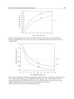
Fig. 5, it is possible to see the impact of OCT in ophthalmology, and also in cardiology, caused
by OCT. That is because of the vacancy of technologies capable to perform images with
resolution good enough to differ between structures, some of them with few microns sized.

Fig. 4. Record count results for “optical AND coherence AND tomography" keyword in the
Web of Science in July of 2010 organized by document type.

Fig. 5. Record count results for “optical AND coherence AND tomography" keyword in the
Web of Science in July of 2010 organized by subject area.
Laser Pulse Phenomena and Applications

412
1.1 OCT concept
The OCT setup it is generally mounted with a Michelson interferometer, and can be divided
in the following main parts: light source, scanning system and light detector, see Fig. 6.
These items define almost all crucial properties of the system. The light emitted from the
light source is divided in two by a beam splitter, part of the beam is directed to the sample
and the other part to the reference mirror, the light backscattered by the sample and the
light reflected by the mirror are recombined at the beam splitter giving origin to an
interference pattern collected by the detector. Because the broadband property of the light
source, the interference pattern will occur only when the optical paths difference between
this two arms are nearly the same. All this process will be discussed in more detail ahead.
The first OCT setup was implemented using femtosecond pulsed laser, due to its broadband
spectral emission (Huang, et al., 1991), which implies in a low coherence length, this feature
is the heart of the OCT system, and the image resolution is correlated to the light source
coherence (as broader the spectral bandwidth, narrower the coherence length will be).

Fig. 6. Schematic representation of an OCT setup.

Fig. 7. Michelson Interferometer.
Optical Coherence Tomography: Development and Applications

413
Nowadays many others light properties are explored too, like polarization sensitive OCT or
Doppler shift OCT are already established, these techniques can extract information about
fiber alignment or particles velocity within the sample, respectively. The efforts by the
research groups for other approaches are being done continuously, since the OCT
development, resulting in ways to extract more information of the sample by the analysis of
the light: Mueller matrix OCT (MM-OCT), pumping-probe OCT (PP-OCT), autocorrelation
OCT, are some examples of OCT approaches in current development.
2. Theory
2.1 Low coherence interferometry
The OCT technique is based on Michelson interferometer (Fig. 7) to produce tomographic
images. A light source, expressed in terms of it electrical field amplitude (equation (1)) is
introduced in the Michelson interferometer and is directed to the beamspliter. It splits the
radiation in two components that are bounded to the reference arm (E
r
) and to the sample
arm (E
s
). Using a beamspliter that divides the beam in two equal parts (50:50), e.g., E
r
and E
s

can be written as equation (2) and (3) respectively.

()
()
ikx t
ffo
Ex Ee
ω
−
= (1)
using 2/k
π
λ
= , 2 /c
ω
πλ
=
and considering just spatial wave propagation

()
()
12
s
ix
c
Sfo
Ex Ee
ω
⎛⎞
⎜⎟
⎝⎠
= (2)

()
()
12
r
ix
c
rfo
Ex Ee
ω
⎛⎞
⎜⎟
⎝⎠
= (3)
The radiation is reflected by the reference mirror, and backscattered by the sample, the
portion of radiation that returns is proportional to the mirror and sample capacity to reflect
and backscatter this radiation. This coefficient R(x), can vary in sample depth (depending on
the sample features). It varies from 0 to 1, where 0 is total transmission and 1 is total
reflection. So, the back reflected and backscattered field (light) suffers an amplitude
modulation. Moreover, the resultant field will be equal to the sum of infinitesimal fields
from different sample depth.
The field comes back to the beamspliter where they are recombined; the field from mirror
and sample are described by equation (4) and (5) respectively. For the mirror R
r
(x)=R
r
δ
(x-x
0
),

where
δ
(x-x
0
) is the Dirac function and x
0
is the mirror position.

()
0
22
0
0
11
()
22
r
ix ix
cc
rr fo r r r for
Ex E R x xe dx ERe
ωω
δ
⎛⎞ ⎛⎞
⎜⎟ ⎜⎟
∞
⎝⎠ ⎝⎠
⎛⎞ ⎛⎞
=−=
⎜⎟ ⎜⎟

⎝⎠ ⎝⎠
∫
(4)

()
()
'
2
''
0
1
()
2
ss
inxx
c
SS
f
oSs s
Ex E Rxe dx
ω
⎛⎞
⎜⎟
∞
⎝⎠
⎛⎞
=
⎜⎟
⎝⎠
∫

(5)
Laser Pulse Phenomena and Applications

414
The factor two in the exponential is to take in account the optical path roundtrip, n(x
S
) is the
refraction index as function of sample depth. The electrical field on the detector (E
D
) will be
a sum of the sample and reference arm electrical fields.

()
0
22
0
11
()
22
ss
ix inxx
cc
DrS
f
or
f
oss s
EEE ERe E Rxe dx
ωω
⎛⎞ ⎛ ⎞

⎜⎟ ⎜ ⎟
∞
⎝⎠ ⎝ ⎠
⎛⎞ ⎛⎞
=+= +
⎜⎟ ⎜⎟
⎝⎠ ⎝⎠
∫
(6)
The intensity on detector (I
D
) is proportional to square modulus of electrical field E
D
:
()
0
2
22
*
0
11
()
22
ss
ix inxx
cc
DDD for foss s
IEE ERe ERxe dx
ωω
⎛⎞ ⎛ ⎞

⎜⎟ ⎜ ⎟
∞
⎝⎠ ⎝ ⎠
⎛⎞ ⎛⎞
∝= + =
⎜⎟ ⎜⎟
⎝⎠ ⎝⎠
∫


() ( )
()
()
()
2''
2
2
00
0
(') ( ) '
2
()cos2
SS S S
inxxnxx
c
rSSSS SS
fo
rS S S S S
R R x R x e dx dx
E

RR x n x x x dx
c
ω
ω
⎛⎞
−−
⎜⎟
∞∞
⎝⎠
∞
−∞
⎡
⎤
⎢
⎥
+
⎛⎞
⎢
⎥
=
⎜⎟
⎜⎟
⎢
⎥
⎛⎞
⎛⎞
⎝⎠
⎢
⎥+−
⎜⎟

⎜⎟
⎢
⎝⎠⎥
⎝⎠
⎣
⎦
∫∫
∫
(7)
At the right side of this equation, the first two terms corresponds to the DC (constant)
intensity from reference and sample arm, respectively, and they do not bring useful
information. The third term is an oscillatory term, and is responsible of bringing information
from the sample to generate OCT images.
Using a broadband spectral source, the equation (7) must be modified in such way that it
comprehends an infinity number of frequencies. The interference only occurs between equal
frequencies, so the total interference will be the sum of the infinitesimal interferences.
()
() ( )
()
()
()
()
2''
2
2
00
0 0
0
(') ( ) '
2

()cos2
SS S S
inxxnxx
c
rSSSS SS
fo
D
rS S S S S
R R x R x e dx dx
E
I dId
RR x nx x x dx
c
ω
ω
ω
ωω
ω
⎛⎞
−−
⎜⎟
∞∞
⎝⎠
∞ ∞
∞
−∞
⎡⎤
⎢⎥
++
⎛⎞

⎢⎥
⎜⎟∝ =
⎢⎥
⎜⎟
⎛⎞
⎛⎞
⎝⎠
⎢⎥+−
⎜⎟
⎜⎟
⎢⎝⎠⎥
⎝⎠
⎣⎦
∫∫
∫∫
∫
(8)
Where I
D
(
ω
) is the intensity on detector for a given
ω
value, and the integral in frequency is
equal to the total intensity on detector I
D
.
The field that comes from reference and sample arm differs only by the optical path, as
expressed by the interference term on equation (7)).
If t is the time that the radiation takes to travel from beamspliter to reference mirror, and t+

τ
is
the time to travel from beamspliter to the scatter position in the sample, so
τ
is the temporal
delay between the two arms. The interference term on equation (7) can be written as:

(
)
2Re
rS
τ
Γ
(9)
Where,

()
*
() ( )
rS r S
T
EtE t
ττ
Γ= + (10)
Optical Coherence Tomography: Development and Applications

415
The Γ
rS
(

τ
) is the coherence function or correlation function between E
r
and E
S
fields. The
function:

()
*
() ( )
SS S S
T
EtE t
ττ
Γ= + (11)
It is known as autocorrelation function. From this definition it is possible to show that
Γ
SS
(0)=I
S
and Γ
rr
(0)=I
r
. For convenience the normalized form of coherence function will be
used, it is called partial coherence degree:

()
(

)
() ()
(
)
00
rS rS
rS
rS
rr SS
II
τ
τ
γτ
ΓΓ
==
ΓΓ
(12)
The
γ
rS
(
τ
) function is, in general, a periodic complex function of
τ
, so the interference pattern
is obtained if the value of |
γ
rS
(
τ

)| is different from zero. The |
γ
rS
(
τ
)| can assume value
between 0 and 1. If the value is equal 1 it says that complete coherence occur, if equal 0 it
says that complete incoherence, for values between 0 and 1 partial coherence occurs.

(
)
1
rS
γτ
=
Complete coherence (13)

(
)
01
rS
γτ
<
< Partial coherence (14)

(
)
0
rS
γτ

=
Complete incoherence (15)
2.2 Time domain
The Fig. 6 shows the basic components of an OCT system. The main part of the system
comprehends an interferometer illuminated by a broadband light source.
The OCT system splits the broadband light source beam in reference field (
E
R
) and a sample
field (
E
S
). They interfere at the detector by summing up the two electrical fields that are
reflected by the optical scanning system (in general a mirror) and the sample. The intensity
in the detector can be expressed by equation (8).
The oscillatory term on equation (8) can also be expressed as:

{
}
'*
Re cos(2 2 )
RS RS RR SS
EE RR l l
ββ
=− (16)
Where
l is the optical path and
β
is the propagation constant (in this case the light source is
highly coherent).

Defining
S(
ω
) = R
S
(
ω
)R
R
(
ω
)* and
Δφ
(
ω
) = 2[
β
S
(
ω
)l
S
-
β
R
(
ω
)l
R
], and considering the case where

the sample and the reference arms consists of a uniform, linear, no dispersive material and
the light source spectral density is given by
S(
ω
-
ω
0
), which is considered to be bandwidth
limited and centered at the frequency
ω
0
. The propagation constants
β
i
(
ω
) in each arm are
assumed to be the same; the diffuse tissue material behaves locally as an ideal mirror
leaving the sample beam unchanged. Propagating the
β
i
(
ω
) coefficient as a first-order Taylor
expansion around the central frequency
ω
0
gives

'

000
() () ( ) ( )( )
RS
β
ωβωβω βωωω
==+ − (17)
Laser Pulse Phenomena and Applications

416
Then the phase mismatch
Δφ
(
ω
) is determined solely by the optical length mismatch
Δ
l=l
S
-l
R

between the reference and the sample arms, and is given by

'
00 0 0
( ) ( )(2 ) ( )( )(2 )ll
φω β ω β ω ω ω
Δ
=Δ+ −Δ (18)
Now, consider that the light source has a Gaussian power spectral density defined by

2
0
2
()
0
2
2
()Se
ω
ωω
σ
ω
π
ωω
σ
−
−
−= (19)
which has been normalized to the unit power. Using this power spectrum and the phase
mismatch is possible to find that detector signal is:

N
2
0
2
0
Re 1
g
p
i

DC
AC
e
Iee
h
τ
τ
τ
ω
σ
βη
Δ
−
−Δ
⎧
⎫
⎪
⎪
∝+
⎨
⎬
⎪
⎪
⎩⎭

  
(20)
In (20), the phase delay mismatch
Δ
τ

p
and the group delay mismatch
Δ
τ
g
are defined as:

0
0p
()
2
(2 )
v
p
l
l
βω
τ
ω
Δ
Δ= Δ= (21)
and

'
0
g
2
()(2)
v
p

l
l
τβω
Δ
Δ= Δ= (22)
The detector signal given by equation (20) contains two terms, the first one is the mean (DC)
intensities returning from the reference and sample arms of the interferometer, and the
second one, which depends on the optical time delay (optical path mismatch) set by the
position of the reference mirror, represents the amplitude of the interference fringes that
carry information about the tissue structure, this is a Gaussian envelope with a characteristic
standard deviation temporal width 2
σ
τ
, that is inversely proportional to the power spectral
bandwidth: 2
σ
τ
=1/2
σ
ω
, This envelope falls off quickly with increasing group delay mismatch
Δτ
g
and is modulated by interference fringes that oscillate with increasing phase delay
mismatch
Δτ
p
. Thus, the second term in equation (20) defines the axial resolving power of
the OCT system. For a Gaussian shape function with standard deviation
τ

, the full width at
half maximum (FWHM) is 2σ√2ln2 then, the axial resolution of the system is:

2
0
2ln2
FWHM
l
λ
π
λ
Δ=
Δ
(23)
where λ
0
is the center wavelength.
2.3 Frequency domain
The Fourier domain optical coherence tomography (FD-OCT) uses a spectrometer, instead a
single detector, to analyze the spectral interference pattern (Fig. 8).
Optical Coherence Tomography: Development and Applications

417

Fig. 8. Michelson Interferometer with a diffractive element an a CCD detector to spectral
measurement.
The equation (7) can be written as a Fourier transform of R
S
(x
S

). To write the equation as a
function of wave number k instead
ω
(equation (24)). There is a correlation between
reciprocal and direct space, given by Fourier transform. It correlates time (s) with frequency
(1/s=Hz) and distance (m) with wave number k (1/m).
()
() ( )
()
()
2
2''
2
00
()
1
(') ( ) ' ()
22
SS S S
iknxxnx x
fo
rSSSS SSzrS
Ek
I k R R x R x e dx dx R R z
−−
∞∞
⎛⎞
⎡⎤
=+ +ℑ
⎡

⎤
⎜⎟
⎢⎥
⎣
⎦
⎜⎟
⎣⎦
⎝⎠
∫∫
(24)
Where z=n(x
S
)x
S
-x
0
is the optical path difference between sample and reference arm. We can
also rewrite the second term as a distance related to the reference mirror.

() ( )
()
()
()
()
()
(
)
00
2''
00

2''
00
(') ( ) '
(') ( ) '
SS S S
SS S S
inxxnxx
c
SSSS SS
iknxx x nx x x
SSSS SS
Rx Rxe dxdx
Rx Rxe dxdx
ω
⎛⎞
−−
⎜⎟
∞∞
⎝⎠
⎡⎤
−−−−
∞∞
⎣⎦
=
∫∫
∫∫
(25)
Substituting z in equation (25), and as the auto correlation is a symmetric function, it has:
[]
()

[]
()
2' 2'
00
11
(')() ' (')() [ (())]'
48
ikzz ikzz
SS SS z S
R z R z e dzdz R z R z e dzdz AutCorr R z
∞∞ ∞ ∞−− −−
−∞ −∞
′
==ℑ
∫∫ ∫ ∫
(26)
Can be identified on this term a Fourier transform, using totally reflective mirror in the
reference arm (R
r
=1), the equation (24) can be rewritten as:
Laser Pulse Phenomena and Applications

418

()
2
()
11
1 [ ( ( ))] ( )
28 2

fo
zSzS
Ek
Ik AutCorrR z R z
⎛⎞
⎛⎞
=+ℑ +ℑ
⎡
⎤
⎜⎟
⎜⎟
⎣
⎦
⎜⎟
⎝⎠
⎝⎠
(27)
For the spectral signal (I(k)) analysis and R
S
(x
S
) information attainment, an inverse Fourier
transform is applied. Finally we obtain:

2
11
()
11
( ) () ( ()) ()
28 2

fo
zz SS
Ek
IK z AutCorrRz Rz
δ
−−
⎡⎤
⎛⎞
⎛⎞
⎢⎥
ℑ=ℑ ⊗+ +
⎡⎤ ⎡⎤
⎜⎟
⎜⎟
⎣⎦ ⎣⎦
⎜⎟
⎢⎥
⎝⎠
⎝⎠
⎣⎦
(28)

(
)
1
()
z
IK A B C D
−
ℑ=⊗++

⎡⎤
⎣⎦
(29)
Using a simplified notation (equations (29)) for equation (28), the R
S
(z) information is
present in convolution of A and C (A⊗C). The convolution A⊗B brings information about
radiation source properties. A⊗D brings information about interference between waves
backscattered in different sample positions. This terms can be ignored for high reflective
medium, since this signal is despicable related to A⊗C term. The signal A⊗B and A⊗D can
be avoided by adequate reference mirror position, a mismatch of few tens of microns avoid
the superposition of A⊗C and the last two terms.
2.3.1 Frequency domain and signal processing
As already discussed in the previous sections, the collected signal in the frequency domain
needs to be processed to form images of interest, i.e., processing the signal will make the
signal direct related with the sample morphology.
Although the processing algorithm has in the core the Fourier Transform to retrieve the
scattering profile (equation (28)), some mathematical manipulations are necessary on the
interferometric pattern due to correction and refinements reasons, aiming images with good
quality. Some of these corrections are necessary due to physical limitation of the equipment,
for example the limited pixel number, or more basic corrections, like changes of unities, for
instance.
Many algorithms can be implemented with different approaches, but this text will be
focused in just three, they are: Direct Fourier Transform (DirFT), Interpolation (Int) and
Zero-Filling (ZF), and they are more detailed explained ahead.
The direct Fourier transform (DirFT) method could be considered as the simpler one,
consequently the more fast and robust. It perform just a change of unity, that is because
spectrometers are calibrated in wavelength, and as OCTs gives information of depth (m), we
need to change from wavelength to wavenumber (k=2
π

/
λ
). This process makes the
spectrum, originally organized in crescent order in wavelength to a reversed order array, so
the vector must to be inverted. After that the vector Fourier transform is done, resulting the
scattering profile. The schematic diagram represents the process Fig. 9 (a). But this process,
i.e., 1/x, cause unequal sized bins, resulting in issues in the Fourier transform, leading to
broadening of the structures and asymmetry of the peaks in respect to the it center. A
method to avoid this problem is to perform an interpolation. After the changing of unities,
the interpolation is done to retrieve equally sized bins, and then submitted to the Fourier
transform, this process is schematic represented in the Fig. 9 (b). The last method (Fig. 9 (c)),
Zero-Filling (ZF) is a technique more elaborated when compared with the two discussed

Optical Coherence Tomography: Development and Applications

419

Fig. 9. Schematic representation of three types of spectral interferometry signal processing
which results in the scattering profile. Between parenthesis dimensional unity.
previously, consequently more expensive computationally. The Zero-Filling technique is
based in a mathematical gimmick, used to increase sampling without increase the data
collection. In practice the (ZF) it is preformed applying the Fourier transform on the
collected spectrum, then, in the reciprocal space, empty arrays (Zero-Filling) are added at
the ends of the original array, the increased sampling of the original data will, according to
the Nyquist theorem, allow to process higher frequencies resulting in less computational
errors (Raele, et al., 2009).
3. Light source
3.1 Light source characteristics
The light source should attend, basically, four main desired characteristics: wavelength,
spectral bandwidth, intensity and stability. Other features could be also listed, as portability,

low cost and etc, but these first four are critical and the reasons for that follows.
First of all the wavelength must be compatible with the sample, mainly because scattering,
absorption and dispersion are wavelength dependent, so if there is interest in measure
inside a sample a wavelength that has low attenuation must be chose. To biological tissue
studies, the region known as “diagnostic window” is often used. This spectral region is
located between 800 nm and 1300 nm.
As shown by equation (23), the spectral band is related with the system resolution, naturally
light sources with broad emission spectral will be preferred, but it is not usual to obtain
broad spectral emission with high intensities. Also it is interesting to highlight that to
maintain a resolution as the wavelength increases, the spectral band also needs to increases,
Laser Pulse Phenomena and Applications

420
for instance an 800 nm with 28 nm of spectral band implies in 10 μm of resolution. To get the
same resolution at 1600 nm the spectral band should be 113 nm.
The intensity of the light source must be intense enough to sensitize the detector giving a
good signal to noise ratio, but as the OCT is often used in biological samples, the intensities
should not overcome the maximum permissible radiation (MPR).
Finally the spectral profile and the intensity must be constant in time; any alteration can
cause issues, like false structures, in the scattering image.
3.2 SLED, mode locked lasers, swept sources
Many kinds of light source can be used in OCT systems, as just they fill in the requirements
described in the previous section, but let us highlight some features of each one of them.
3.2.1 Super iuminescent LED (SLED)
The SLED it is, perhaps, the most popular OCT light source nowadays due to its low cost
and easiness of handling. It presents intensities high enough to perform tomographic
images, and also presents high spectral stability. Another good thing about it is that is
possible to acquire it pigtailed (connected to an optical fiber). The drawbacks are limited
spectral band, about 30 nm and intensities not high enough to perform extremely fast
scanning.

3.2.2 Lasers
Lasers, usually, are applied in OCT research, most of them using a Ti:Sapphire laser system
operating in mode locked regime, because in this kind of operation a broadband radiation is
promoted. Lasers are a most flexible, about spectrum and intensity, then system with SLED.
Without doubt the major drawbacks of applying mode locked lasers is the cost.
Lasers systems allows intensities high enough to perform images at so high rates, in this
way, the involuntary movements of the live system that are under study do not affect the
image.
Mode locked lasers also can be used to generate a supercontinuum spectra by injecting it in
a photonic fiber. In this type of fibers, nonlinear effects produces spectra large as 400 nm,
allowing submicron of spatial resolutions.
3.2.3 Swept source
A Swept Source is a broadband laser with an intracavity optical narrowband filter. Only
longitudinal modes with the exact frequency selected by the filter can oscillate, so the laser
action occurs on a single frequency. This filter can be frequency tuned, sweeping the
frequency laser action. The filtering tune is made so all the laser spectral frequencies be
tuned on the photon cavity roundtrip. The output laser is not a sort pulse train, as a mode-
locked laser, but a tuned frequency train with long pulses. The tuned frequencies have the
same phase evolution and they are coherent between each other.
4. Scanning systems
Before entering in the subject itself, let us stress to the reader that is more than one type of
scanning, usually we need a lateral scan and also a depth scan, be sure that are clear in mind
before continue. The lateral scan can be easily done with a galvanometric system or even a
Optical Coherence Tomography: Development and Applications

421
linear translator that moves a sample perpendicularly to the incident light beam. Below are
discussed the depth scan, also known as A-scan and have two different approaches to be
performed: Time Domain and Frequency Domain, as detailed in the theory section, the
issue, now, it is how to perform in practice this two types of A-scan.

4.1 Time Domain
In Time Domain OCT the optical path of the reference arm needs to vary in time so the
scattering profile, of a single point of the sample, can be recorded. Change the optical path of
an interferometer arm can be done with simple systems, simple as a mirror fixed in a speaker,
of course that is not the most reliable and faster way, but it will do. When systems with more
finesse are required more complex systems are needed. That are many type of scanning
system, when using optical fibers, to stretch it with kHz repetition, usually, can be done using
a piezoelectric device. This configuration assures high mechanical stability due to the use of
the optical fiber. Another configuration reported is to place a rotating glass cube between the
beam splitter and the mirror. As the cube rotates the optical path changes due to refraction,
with this setup was achieved the A-scanning record (Bouma, et al., 2002), another used
configuration is kwon as Fast Fourier Scanning (FFS) scanning, also achieves high repetition.
4.1.1 Frequency Domain
The main advantage of Frequency Domain OCT it is that, once that a CCD based
spectrometer is used, there is no need of any mechanical variation in time. All the depth
information, the scattering profile, is encoded in the spectral interference pattern, which can
be recorded easily with the help of a personal computer. So in this case the reference arm
stands still. In the other hands, as drawbacks about, about the FD-OCT, is the detector cost
and complexity, still, is the configuration more used in commercial systems. Another issue
to be mentioned is that FD signal needs more processing, i.e., more powerful computers.
4.1.2 Swept source
The swept source can be understood as a characteristic FD approaches, but due to the source
features the spectrum is acquired as a function of time. There is a relationship between time
and wavelength. Also the signal acquired needs to be processed in the same way that in the
FD-OCT. So, what is the catch? Well, now the cost of having a spectrometer is avoided, in
SS-OCT a single photo-detector is used (no gratings, no moving mirrors and CCDs).
Mechanically the SS setup has no moving parts, as FD, which is a very desirable feature,
however, in the SS system the swept source itself it has a high cost and complexity.
The Swept source applied to OCT (SS-OCT) allows images construction between 10 to 50
times quiker than traditional OCT and, due to SS be a laser, the SS intensity is greater than

superluminescent LED, allows deeper tissue penetration.
5. PS-OCT
Light exhibits polarization states; due to the property that light vibrates orthogonally in
respect to the propagation direction. Measure change in polarization in many cases can be
considerate relatively simple process, but measure change in polarization as position
function (inside a sample) it is not trivial. Using an OCT system it is possible to gather
information from different polarizations states and perform not a scattering image, but it is
Laser Pulse Phenomena and Applications

422
possible to perform birefringence images (Hee, et al., 1992). PS-OCT needs some
modification in the setup (Fig. 10), a polarized light source a polarization analyzer and a
pair of quarter wave plate is needed.

Fig. 10. Diagram to PS-OCT, a linear polarized light is spliced in two parts, in the sample
arm the polarization is rotated to 45º, and in the sample arm is converted in circular
polarized. The detector register the two orthogonal polarized light depending of the
analyzer angle.
The polarized light hits the beam splitter, then a fraction is transmitted and other is
reflected. Looking for the sample arm, one can think that the linear polarized light could be
aligned with one optical axis of the sample (fast or slow axis) which would result a ordinary
OCT scattering image, to avoid that a quarter wave plate, at 45°, is placed before the sample,
causing a circular polarization state, in this way the light can be not aligned with any optical
axis. The sample will cause some backscattering; the light will then, again, pass through the
quarter wave plate. Remembering that the light has passed twice through the quarter wave
plate at 45°, the light will return to the beam splitter with a linear polarization state rotated
of 90° in respect of the original polarization state (light source).
So in the sample arm the light already contain all the information that is needed, the issue is
now on the reference arm, that is because due to the reason that light interfere only when
both beams have components of the same polarization state, i.e., a horizontally and a

vertically polarized will not interfere, but a horizontally and a 45° polarized light will have a
interference because the 45° state of polarization it is a superposition of vertical and
horizontal polarization, and in this way will present interference pattern over a DC
component. The polarization properties of the light can provide crucial information about
the sample structure, and analyzing the polarization properties of a sample by the
backscattered light as depth function allow to measure biological tissues and many other
materials with strong scattering.
With a Polarization Sensitive OCT birefringence images can be performed (Fig. 11), in this
way the differences between the refraction indices can be analyzed as an image, making
diagnoses simple to be performed (Raele, et al., 2009).
Optical Coherence Tomography: Development and Applications

423

Fig. 11. Birrefringent image with PS-OCT of an adhesive tape, the birefringence of this tape
was measured as 4.03(26)x10
-4

Besides PS-OCT images, a more complex, but also more complete way to study the
polarization properties of light can be done using the Mueller Matrix theory (Bickel, et al.,
1985).
5.1 Doppler OCT
A number of extensions of OCT capabilities for functional imaging of tissue physiology
have been developed. Doppler OCT (Chen Z, et al., 1997), also named optical Doppler
tomography (ODT), combines the Doppler principle with OCT to obtain high-resolution
tomographic images of tissue structure and blood flow simultaneously (Fujimoto, et al.,
2008). The Doppler OCT combine a technique developed in the 60´s, the Doppler
velocimetry, with the traditional OCT high resolution images, mapping the fluids velocity
and their localizations in the tissue open a new frontier as a diagnostic tool.
Considering the referential frame moving with a velocity

v in this referential the frequency
of light will be:
0
1
2
i
fKv
π
−
⋅ (Fig. 12 (b)), and the scattered light field will be described by:
The light frequency scattered by a moving object will be
0
2( ).
is
f
tKKv
π
−
−⋅ In a Doppler
OCT experiment the light and the scattered light share the same optical path in the sample
arm like in (Fig. 12 (a)).
The Doppler shift can be determined measuring the phase shift between two consecutive
spectra for A-scan, since in SD-OCT the A-scan are calculated with complex functions
(Brezinski, 2006).

()
()Re[ ()] () ()
iz
DD DD
iz Iz iImIz ize

φ
′
′
⎡⎤
′′ ′′ ′′ ′′
=+ =
⎣⎦


(30)
The phase of this complex function is the phase information of each A-scan described as:

[()]
( ) arctan
[()]
D
D
Im i z
z
Re i z
φ
⎧
⎫
′
′
⎪
⎪
′′
=
⎨

⎬
′
′
⎪
⎪
⎩⎭


(31)
the phase shift
Δφ
(z´´) can be used to obtain the Doppler velocity.

00
()
4()cos
D
z
V
Tknk
φ
π
θ
′
′
Δ
= (32)
Laser Pulse Phenomena and Applications

424

Fig. 12. (a) Diagram of Doppler-OCT and (b) the change in the wavelength of scattered light
from a moving particle
6. Applications
6.1 Ophthalmology
OCT systems found it first application performing retina tomographies (Huang, et al., 1991),
this was the beginning of what have become a revolution in the ophthalmology area, OCT
allowed the specialists to exams the eye as the same way of histology does, but in a completely
non invasive, non traumatic and painless way and also in real time. Latter OCT image
resolution and depth characteristics matches the needs of ophthalmologists and the eye itself,
especially when the OCT is operating at the NIR region, which has low attenuation and does
not sensibilizes the vision cells. Besides retina the specialists also use OCT to examine the eye
anterior segment and cornea, see Fig. 13. Nowadays OCT is routine in many ophthalmic clinics
around the world, and researches are improving this tool continuously.
Diseases as glaucoma and retinal dystrophy among many other examples (Schuman, et al.,
2004) can be diagnosed using OCT systems, some of them were a complicated issue to
diagnoses, as macular degeneration, has now the OCT as a primary way to do it.


Fig. 13. Image of a mice cornea. The arrow indicates the place where a thickness of it was
evaluated.
Optical Coherence Tomography: Development and Applications

425
In terms OCT improvements, some outstanding studies has being done, for instance
reported 3 μm of resolution (Wampler), this is refined enough to actually “see” the retina
cells. The possibilities of applications are many, monitoring LASIK proceedings, study the
blood flux, etc.
6.2 Dermatology
OCT also caused a significant impact dermatology for almost the same reasons that

promoted OCT in ophthalmology. As shown in Fig. 1, OCT technique can perform images
where is possible to indentify the different skin structures ( A. stratum corneum; B.
epidermis; C. dermis and D. Sweat gland), researches are studing many features of skin in
vivo, impossible feat before OCT.
Diseases, even skin cancer, can be diagnosed by this tool (Mogensen, et al., 2009). Skin has
been studied extensively also with PS-OCT (Hee, et al., 1992), that is because many
compounds in skin presents birrefringence and the concentration of this compounds are
related with skin health.
6.3 Odontology
In odontology, a series of reports first appeared (Colston, et al., 1998), (Feldchtein, et al.,
1998) in 1998, with imaging of both hard and soft oral tissues. This led to several diagnostics
of bucal diseases, including periodontal, early caries, among others. Another area in
dentistry where OCT can have important findings is in dental restoration imaging.(Wang, et
al., 1999), (Fried, et al., 2002), (Otis, et al., 2000), (Jones, et al., 2004), (Wang, et al., 1999) and
(Fried, et al., 2002) exploited polarization-sensitive OCT to identify dental tissue/restoration
interfaces. To date, there is no quantitative method capable to perform in vitro or in vivo
analysis of dental restoration, particularly from the clinical point of view. Visual inspection
and X-ray imaging are not precise enough to diagnose small gaps that result from bad
restoration procedures. Dental tissues are high scattering media and infrared light can
penetrate the full enamel extension (Fried, et al., 1995).
Although, in odontology, OCT is not yet broadly available, as in ophthalmology, the
potential of the technique promises a fast technological development that requires more
laboratory evaluation, prior to clinical trials.
One of important area of interest is the restorative procedures, the application of OCT to
dental restoration, particularly analyzing failure gaps left after the restoration has been
performed (Melo, et al., 2005).
Another import field of interest is the dental caries, and this disease is known as a
multifactorial pathological process, characterized by hard tissue demineralization.
Commonly, dentists evaluate the oral health of a patient through three main methods:
visual, tactile examination and radiographic imaging (Bosh, 1993). The visual method

cannot detect early caries lesion and depends of the dentist ability to identify these lesions.
There are many caries detector dyes commercially available purported to assist the dentist
in differentiation of infected tissue, but they are not specific and would result in
unnecessary removal of healthy tooth structure (McComb, 2000). OCT in dentistry has been
recently used to in vitro studies evaluating enamel interface restoration (Melo, et al., 2005),
early caries diagnostics (Freitas, et al., 2006), and analysis of the performance of dental
materials (Braz, et al., 2009). In 2006, the first OCT image of dental pulp was performed
using rat’s teeth (Kauffman, et al., 2006), and more recently, remaining dentin and pulp
chamber from human’s teeth were also imaged by OCT in vitro (Fonseca, et al., 2009).
Laser Pulse Phenomena and Applications

426
The OCT can detect and quantify demineralization (FREITAS, et al., 2009). The Fig. 14 (a)
shows an OCT image for a sample submitted to the demineralization process for 11 days,
and in (b) the 3D image reconstruction.
The OCT system provides a powerful contact less and noninvasive diagnostic method that
could be used to complement the traditional diagnostic methods such as X-ray radiography,
avoiding potentially hazardous ionization radiation.
Polarization-sensitive optical coherence tomography (PS-OCT) is potentially useful for
imaging the nonsurgical remineralization of dental enamel. The PS-OCT can image the
effects of mineralization status and scattering properties of dental caries (Jones, et al., 2006),
(Baumgartner A, et al., 2000).


Fig. 14. (a) Transversal OCT image after the sample was submitted to the demineralization
process for 11 days and (b) 3D image reconstruction allows another image sections analysis
different from those obtained directly from the OCT system.
6.4 Non-biomedical applications
Despite the wide use of OCT for biological application, it noninvasive and nondestructive
features are very attractive in other areas. The use of OCT technique has grown on art and

cultural heritage artifacts studies (Targowski, et al., 2006) (Liang, et al.), e.g., for investigate
various art objects such as oil paintings, see Fig. 15 and Fig. 16, on canvas to image
pigments, glaze and varnish layers (Rouba, et al., 2008 ) or historical coins (Amaral, et al.,
2009) for instance.



Fig. 15. Image of oil painting with varnish layer
Optical Coherence Tomography: Development and Applications

427



Fig. 16. Image of oil painting over sketch made with pencil.
It has been also used also for investigate wood from musical instruments structures, as
fibers, rays, cell wall distribution. As well as varnished wood: morphological properties,
such roughness, interfaces, and thickness; and compositional properties, such shape, size,
distribution of pigments and fillers. And even more, understanding of the penetration of the
varnish inside the wood or the wear processes of these materials, applying these kinds of
study on a 18th century Italian violin (Latour, et al., 2009).
OCT finds on industry another field of actuation, due to the real time and noncontact
feature. Moreover, some traditional technique, used in the industry, cannot be applied to
some materials. For e.g., to measure textile roughness, see Fig. 17, traditional technique to
roughness measurement, that uses contact cantilever, could cause erroneous values and
even damage the textile. Is reported the development of a methodology and algorithm to
give metrological parameter of roughness according DIN4768 (Amaral, et al., 2009), that can
be applied to delicate samples. Applications also can be found in printed electronics
products quality (Czajkowski, et al., 2010) and in paper industry (Prykär, et al., 2010).

Fig. 17. OCT images can be used to perform roughness measurements without contact.
6.5 Dermatology
OCT also caused a significant impact dermatology for almost the same reasons that
promoted OCT in ophthalmology. As shown in Fig. 1, OCT technique can perform images
where is possible to indentify the different skin structures, researches are studing many
features of skin in vivo, impossible feat before OCT.
Laser Pulse Phenomena and Applications

428
Diseases, even skin cancer, can be diagnosed by this tool (Mogensen, et al., 2009). Skin has
been studied extensively also with PS-OCT (Hee, et al., 1992), that is because many
compounds in skin presents birrefringence and the concentration of this compounds are
related with skin health.
Another important subject in dermatology is cosmetic science, which claim for a non
invasive method to efficiency evaluation of anti-aging or anti-wrinkle products, for instance.
Hair is a substructure of skin and it also can be studied with OCT. Fig. 18 (a) shows the
cross-sectional image of Afro-Ethnic hair, where is possible to identify two hair structures:
medulla and cortex (Lademann, et al., 2008), (Velasco, et al., 2009). The tridimensional image
(Fig. 18 (b) was built starting from 601 cross-sectional images (slices) like Fig. 18 (a).




Fig. 18. OCT image of an Afro-Ethnic hair sample. In (a) a sample of cross-section fiber and
at (b) a tridimensional reconstruction of that fiber, showing the main hair structures:
medulla, cortex and cuticle.
8. Conclusions

Using broadband light sources, as mode locked lasers, in an interferometric setup allows
perform tomographic images with high resolution and non invasive way. This technique,
known as optical coherence tomography (OCT), found, in many areas of knowledge, great
potential. Worth mention that in ophthalmology OCT promoted a revolution in the way that
diagnoses are performed.
Although OCT is a relatively new technique, created in 1991, the applications and more
powerful and versatile systems are increasing rapidly in number.
9. References
A Baumgartner [et al.] Polarization–Sensitive Optical Coherence Tomography of Dental
Structures [Artikel] // Caries. Res - 2000 . - Bd. 34.
Amaral Marcello M. [et al.] “Roughness measurement methodology according to DIN 4768
using optical coherence tomography (OCT) [Konferenz] // Proc. SPIE. - Munch :
Spie, 2009. - Bd. 7390.
Optical Coherence Tomography: Development and Applications

429
Amaral Marcello M. [et al.] Laser induced breakdown spectroscopy (LIBS) applied to
stratigrafic elemental analysis and optical coherence tomography tomography
(OCT) to damage determination of cultural heritage Brazilian coins [Konferenz] //
Proc. SPIE / Hrsg. Spie. - Munch: Spie, 2009. - Bd. 7391.
Andrew M. Rollins Siavash Yazdanfar, Jennifer K. Barton, Joseph A. Izatt, “ Real-time in
vivo color Doppler optical coherence tomography [Artikel] // J. Biomed. Opt -
2002. - S. Vol. 7, 123.
Baumgartner A Dichtl S, Hitzenberger C K [et al.] Polarization–Sensitive Optical Coherence
Tomography of Dental Structures [Artikel] // Caries. Res - 2000. - Bd. 34. - S. 59-
69.
Bickel W.S. und Bailey W.M. Stokes vectors, Mueller matrices, and polarized scattered light
[Artikel] // Am. J. of Phys - 1985. - S. v.53, n.5, p. 468-478.
Bosh B. Angmar-Mansson and J.J. Ten Optical Methods for the Detection and Quantification
of Caries [Artikel] // Adv. Dent. Res. - 1993. - Bd. 7. - S. 70–79 .

Bouma Brett E. und Tearney Guillermo J. Handbook of Optical Coherence Tomography
[Buch]. - NY : Marcel dekker Inc, 2002.
Braz A.K.S. [et al.] Evaluation of crack propagation in dental composites by optical
coherence tomography [Artikel] // Dent. Mater - 2009. - Bd. 25. - S. 74-79.
Brezinski Mark E. Optical Coherence Tomography, Principles and Applications [Buch]. -
Oxford : Elsevier Inc., 2006.
Chen Z Milner T, Dave D und Nelson [Artikel] // J. Opt. Lett - 1997. - S. 22 64–6.
Colston B. W. [et al.] Dental OCT [Artikel] // Opt. Express. - 1998. - Bd. 3. - S. 230-238.
Colston B. W. [et al.] Imaging of hard-and soft-tissue structure in the oral cavity by optical
coherence tomography [Artikel] // Appl. Opt - 1998. - Bd. 37.
Czajkowski Jakub [et al.] Optical coherence tomography as a method of quality inspection
for printed electronics products [Artikel] // Opt.l Review. - 2010. - 3 : Bd. 17. - S.
257-262.
Eden Alec The search for Christian Doppler [Buch]. - Wien : Springer-Verlag, 1992.
Feldchtein F. I. [et al.] In vivo OCT imaging of hard and soft tissue of the oral cavity
[Artikel] // Opt. Express. - 1998. - Bd. 3. - S. 239-250.
Fercher A. F. [et al.] In vivo optical coherence tomography [Artikel] // Amer. J.
Ophthalmol - 1993. - S. v.116, pp. 113-114,.
Fonseca D.D.D. [et al.] [Artikel] // J. Biomed. Opt - 2009. - Bd. 14. - S. 024009.
Freitas A. Z. [et al.] Imaging carious human dental tissue with optical coherence
tomography [Artikel] // J. Appl. Physics. - 2006. - 024906 : Bd. 99.
FREITAS A.Z. [et al.] Determination of dental decay rates with optical coherence
tomography [Artikel] // Laser Physics Letters. - 2009. - Bd. 6. - S. 896-900.
Freitas A.Z. [et al.] Imaging Carious Human Dental Tissue with Optical Coherence
Tomography [Artikel] // Journal of Applied Physics. - 2006. - S. v. 99, n.2, p.24906.
Fried D. [et al.] Nature of light scattering in dental enamel and dentin at visible
and nearinfrared wavelengths [Artikel] // Appl. Opt - 1995. - Bd. 34. - S. 1278–
1285.
Laser Pulse Phenomena and Applications

430
Fried D., Shafi S. und Featherstone J. D. B. Imaging caries lesions and lesion with
polarization sensitive optical coherence tomography [Artikel] // J. Biomed. Opt -
2002. - Bd. 7. - S. 618–626.
Fujimoto J. G. und Drexler W. Optical Coherence Tomography [Buchabschnitt]. - Berlin :
Springer, 2008.
Goode B.G. Optical Coherence Tomography: OCT aims for Industrial Applications
[Online]. - 10. 9 2008. - 10. 9 2008. –
/>OPTICAL-COHERENCE-TOMOGRAPHY:-OCT-aims-for-industrial-application.
Hee M. R. [et al.] Polarization-sensitive low-coherence reflectometer for birefringence
characterization and ranging [Artikel] // J. Opt. Soc. Am B. - 1992. - S. v. 9, p. 903-
908.
Hee M.R. [et al.] Optical coherence tomography of the human retina [Artikel] // Arch.
Ophthalmol - 1995. - S. Vol. 113, pp.326-332.
Huang D. [et al.] Optical Coherence Tomography [Artikel] // Science. - 1991. - 1178 : Bd.
254.
J. Wang T. E. Milner, and J. S. Nelson Characterization of fluid flow velocity by optical
Doppler tomography [Artikel] // OPTICS LETTERS. - 1995. - S. Vol. 20, No. 11 /
1337-1339.
Jones R. S., Staninec M. und Fried D. Imaging artificial caries under composite sealants and
restorations [Artikel] // J. Biomed. Opt - 2004. - Bd. 9. - S. 1297–1304 .
Jones Robert S. [et al.] Remineralization of in vitro dental caries assessed with polarization-
sensitive optical coherence tomography [Artikel] // Journal of Biomedical Optics. -
2006. - 1 : Bd. 11. - S. 014016.
Jones Robert S. [et al.] Remineralization of in vitro dental caries assessed with polarization-
sensitive optical coherence tomography [Artikel] // Journal of Biomedical Optics. -
2006. - 1 : Bd. 11.
Kato I. T. [et al.] Inhibition of enamel remineralization with blue LED: an in vitro study
[Konferenz] // Proc. of Spie Lasers in Dentistry XV. - San José : Spie, 2009. - S. v.
7162.

Kauffman C.M.F. [et al.] [Konferenz]. - [s.l.] : Proc. SPIE, 2006. - 613707 .
Lademann J. [et al.] Application of optical non-invasive methods in skin physiology
[Artikel] // Laser Phys. Lett - 2008. - 5 : Bd. 5. - S. 335-346.
Latour Gaël [et al.] Structural and optical properties of wood and wood finishes studied
using optical coherence tomography: application to an 18th century Italian violin
[Artikel] // Applied Optics. - 2009. - 33 : Bd. 48. - S. 6485-6491 .
Liang Haida [et al.] 2. En-face optical coherence tomography: a novel application of non-
invasive imaging to art conservation [Artikel] // Optics Express. - 16 : Bd. 13. - S.
6133-6144 .
Martinez O. E. 3000 times grating compressor with positive group velocity dispersion:
Application to fiber compensation in 1.3-1.6 pm regime [Artikel] // O. E. Martinez,
IEEE J. Quantum Electron. QE-23, 59 (1987) - 1987. - Bde. QE-23.
McComb D. Diagnoses of occlusal caries [Artikel] // J. Can. Dent. Assoc - 2000. - Bd. 66. -
S. 195–198 .
Optical Coherence Tomography: Development and Applications

431
Meirelles R.L., Aggio F.B. und Costa R.A. STRATUS optical coherence tomography in
unilateral colobomatous excavation of the optic disc and secondary retinoschisis
[Artikel] // Graefes Archive For Clinical And Experimental Ophthalmology. -
2005. - S. V. 243, n. 1, p. 76-81.
Melo L. S. A. [et al.] Evaluation of enamel dental restoration interface by optical coherence
tomography [Artikel] // Journal of Biomedical Optics. - 2005. - S. v.10, n.6,
p.1-5.
Mogensen Mette [et al.] OCT imaging of skin cancer and other dermatological diseases
[Artikel] // Journal of Biophotonics. - 2009. - 6-7: Bd. 2. - S. 442 - 451.
Otis L. L. [et al.] Identification of occlusal sealants using optical coherence tomography
[Artikel] // J. Clin. Dent - 2000. - Bd. 14. - S. 7–10.
Prykär Tuukka [et al.] Optical coherence tomography as an accurate inspection and quality
evaluation technique in paper industry [Artikel] // Opt. Review. - 2010. - 3 : Bd.

17. - S. 218-222.
Raele Marcus Paulo and Freitas Anderson Zanardi Desenvolvimento de um sistema de
tomografia por coerência óptica no domínio de Fourier sinsível á polarização e sua
utilização na determinação das matrizes de Mueller [Report]. - São Paulo : Instituto
de Pesquisas Energéticas e Nucleares IPEN-CNEN/SP, 2009.
Rouba Bogumiła J. [et al.] Optical coherence tomography for non-destructive investigations
of structure of objects of art [Konferenz] // 9th International Conference on NDT of
Art. - Jerusalem : [s.n.], 2008 .
Schuman Joel S., Puliafito Carmen A. and Fujimoto James G. Optical Coherence
Tomography of Ocular Diseases [Book]. - NJ : SLACK, 2004.
Shuliang J., Gang Y. und Lihong Depth-resolved two-dimensional Stokes vectors
of backscattered light and Mueller matrices of biological tissue measured with
optical coherence tomography [Artikel] // Appl. Opt - 2000. - S. v. 39, n. 34, p.
6318-6324.
Targowski Piotr, Góra Michalina und Wojtkowski Maciej Optical Coherence Tomography
for Artwork Diagnostics [Artikel] // Laser Chemistry. - 2006. - Bd. 2006.
Tearney G. J., Bouma B. E. und Fujimoto J. G. High-speed phase- and group-delay scanning
with a grating-based phase control delay line [Artikel] // Opt. Lett - 1997. - Bd. 22.
Velasco Maria Valéria Robles [et al.] Prospective ultramorphological characterization of
human hair by optical coherence tomography [Artikel] // Skin Research and
Technology. - 2009. - Bd. 15. - S. 440-443.
Wampler Steve OCT News [Online] // OCT News. - 30. 07 2010. –

Wang X. J. [et al.] Characterization of dentin and enamel by use of optical coherence
tomography,” , () [Artikel] // Appl. Opt - 1999. - Bd. 38. - S. 2092–2096.
Web of Science [Online] // Web of Science. - 7 2010, 7. –

Zhongping Chen Thomas E. Milner, Digant Dave. und Nelson J. Stuart Optical Doppler
tomographic imaging of fluid flow velocity in highly scattering media [Artikel] //
Optics Letters. - 1997. - S. Vol. 22, Issue 1, pp. 64-66.

Laser Pulse Phenomena and Applications

432
Zhongping Chen Thomas E. Milner, Shyam Srinivas, Xiaojun Wang, Arash Malekafzali,
Martin J. C. van Gemert, and J. Stuart Nelson Noninvasive imaging of in vivo blood
flow velocity using optical Doppler tomography [Artikel] // Optics Letters. - 1997. -
S. Vol. 22, Issue 14, pp. 1.
21
High Resolution Biological
Visualization Techniques
Pavlina Pike
1
, Christian Parigger
2
and Robert Splinter
3

1
University of Alabama at Birmingham
2
University of Tennessee Space institute
3
University of North Carolina at Charlotte
USA
1. Introduction
Imaging with ionizing radiation is an integral part in today’s medicine. For example, breast
tissue is more radiosensitive during puberty and exposures to the chest during that time
would impose a higher risk of radiation-induced breast cancer (Doody et al., 2000). The use
of ionizing radiation for medical imaging has significantly increased in the past 20 years,
which has caused the effective dose per individual in the US to increase from 0.53 mSv in

the early 1980s to 3 mSv in 2006 as reported by the National Council on Radiation Protection
and Measurement. [NCRP No. 160, 93] This has naturally raised concerns about the possible
risks that are associated with multiple exposures from diagnostic sources of radiation. There
is a huge effort towards creating imaging modalities that can visualize tissue with a reduced
dose to the patient without loss of image quality. Therefore, it would be advantageous to
develop visualization techniques that employ non-ionizing radiation and that provide
comparable high-resolution image quality as the currently available modalities. This is one
reason why Magnetic Resonance Imaging (MRI) technology is gaining so much popularity
in spite of the cost and the length of the exams.
The non-invasive nature of light in the near-infrared region and its reduced attenuation in
tissue are the reasons why optical imaging is gaining popularity. However, tissue scatter is a
major limitation in optical imaging techniques. It is possible to combine optical imaging and
ultrasound to produce images. This is accomplished by the use of ultra-short laser pulses
that are absorbed in the medium, which cause the temperature of the material to rapidly rise
and fall. Consequently, the irradiated volume becomes an internal source of ultrasonic
waves, which can be used to obtain diagnostic information. Photo-acoustic spectroscopy has
been shown to be a great tool to successfully visualize and characterize:
• blood vessels (Zhang et al. 2009; Hoelen et al. 1998; Sethuraman, S. et al. 2006);
• breast cancer (Ermilov et al. 2009);
• brain in vivo (Wang, X. D. et al. 2003; Yang, X. et al. 2007; Lingu et al. 2007);
• prostate lesions (Yaseen et al. 2010).
Photo-acoustic spectroscopy has also been considered for detection of caries in its early
stage (Kim et al. 2006), analysis of dental materials (Coloiano et al. 2005) and potentially for
visualizations under porcelain crowns. (Pike et al. 2007) New clinical demands for imaging
are continuously emerging, placing different constraints on the imaging requirements and
Laser Pulse Phenomena and Applications

434
the imaging conditions, e.g., in-vivo versus in-vitro imaging. One such new development in
biology is regenerative medicine, which addresses cell structure growth for transplant

purposes. In regenerative medicine the organ is grown outside the body and requires
quality control before it can be implanted in a living organism with a high degree of success
for survival (Hendee W et al., 2008).
2. Examples of available imaging applications
The visualization of superficial vascular malformations, for instance has been shown to
benefit most from thermography (Saxena AK, Willital GH, 2008). Another example is in
dentistry: Dental X-ray images are problematical for clear display of the vitality of dental
pulp, especially under ceramic crowns. Such an evaluation is important, because severe pain
can originate from the pulp as a result of trauma or dental caries. In addition, for patients
undergoing a hart valve replacement surgery or cancer patients undergoing treatment while
on immunosuppressant medication such infections can be life threatening (Pike P et al.,
2007).
Optical Coherence Tomography (OCT) can be applied in various formats, using the
respective optical characteristics of laser- light: coherence, spectral compositions,
polarization and time-of-flight. The specific OCT applications available are for instance:
Time domain OCT; Frequency domain OCT (FD-OCT); Polarization-sensitive OCT; spatially
encoded frequency domain OCT (spectral domain or Fourier domain OCT); and time
encoded frequency domain OCT (also swept source OCT) in addition to combinations of
their mechanisms. Each application reveals its own particular details about the tissue
composition, pathological conditions and structural formation (Huang SA et al., 2007).
Microwave images use Giga Hertz electromagnetic radiation to interact with the cellular
structure on an electronic level (Fear EC et al., 2002).
Microwave imaging uses the fact that cells show dipole character with a membrane that act
as independent electronic circuits. The electronic tissue details can provide histological and
pathological information non-invasively and in-vivo. The mechanism of action relies on the
cellular components’ dielectric properties that will influence the wave propagation and
hence act as a sensing mechanism (Semenov et al., 1995, Semenov et al., 1996).
Spectroscopic imaging for all wavelength ranges uses the alteration in the spectral structure
of the input signal both in the time and frequency domain as a result of interaction with the
biological medium. Time-resolved spectroscopy is gaining popularity as a result of the

reduced price of sensors that are capable of the high speed, short-time response (femto-
second) as well as the reduced size of the sensors.
In optical, microwave and acoustic imaging techniques the spectral performance will embed
crucial tissue information. However, the most accurate spectral application of Raman
spectroscopy can primarily be realized free-space since the delivery device usually
introduces its own Raman spectral aberrations. In this case time-resolved spectroscopy may
offer a solution for all non-ionizing imaging techniques.
The purpose of this chapter is to summarize both in-vivo and in-vitro techniques that
involve image formation based on signals generated in tissue by the various visualization
methods applying non-ionizing radiation for high-resolution signal generation and
sensing/imaging. In this chapter three high resolution imaging techniques will be described
each relying on the time-of-flight principle in various formats [both acoustic and optical]
and the available options to enhance the level of detail that can be resolved. The importance
High Resolution Biological Visualization Techniques

435
of high resolution imaging for diagnostic clinical and laboratory applications is illustrated
by the imaging requirements which is followed by the detailed description of the scientific
basis of Photo-Acoustic imaging (PAI) and several potential applications, followed by the
mechanism of action of ultra short laser pulses, generally crucial to the photo-acoustic
technique that are particularly critical to establish non-destructive testing conditions.
Additionally the coherence aspect of time-of-flight is described with Optical Coherence
tomography and the available options within this technique. The chapter will conclude with
a description of short-pulse measurements and in particular application of autocorrelation
measurements from interference images.
3. Biological imaging requirements
One possibility is to generate acoustic waves with femto-second laser pulses and analyze the
recorded signals. This process is called Photo-Acoustic (PA) spectroscopy and has been
shown to be highly sensitive for variety of applications, including the determination of
small concentrations of molecular species, and the analysis of photo-thermal expansion and

contractions of molecules. One advantage of such techniques is that the signal generation is
primarily a result of the absorption of electromagnetic radiation inside the tissue. Scattering
is not a major factor in the signal degeneration. This method has been shown to be useful to
detect breast cancer (Ermilov SA et al., 2009), to visualize vasculature in mouse brain by
adding golden nano-spheres to improve optical contrast (Lu W et al., 2010), to evaluate
tissue growth and regeneration (Yuan Z et al., 2010), and 3-D visualization blood vessels
(Zhang EZ et al., 2009). In fact different variations of this technique have been developed for
specific clinical applications.
The advantage of the PA technique is that the signal is generated primarily as a result of the
absorption of light. Distortion of the signal due to scattering is not an issue as in other imaging
methods. Recently, it has been shown to be viable for variety of biomedical applications, such
as visualization of tumor angiogenesis and characterization of arterial walls.
4. Photo-acoustic spectroscopy
4.1 Photo-acoustic imaging mechanism of action
It was Alexander Bell who reportedly first described the phenomenon of sound generation
in materials by light (Bell, 1880). As he shone chopped light on strongly absorbing
substances he observed that audible sound was generated. Todays laser systems can deposit
energy via ultra short optical pulses and cause the rapid thermal expansion and relaxation
of the targeted volume in the tissue. That in turn will cause the generation of a pressure
wave which will carry information about the thermal and mechanical characteristics of the
tissue in which it originated. The ultrasonic wave is then detected by the use of a transducer
or an array of transducers for parallel data acquisition.
The energy deposited by the laser puse will be absorbed and and then it will diffuse into the
surroundings. The temperature will initially spike and then a gradual decrease will follow.
The time it takes for it to reach 37% of its original value is called the thermal relaxation
time, defined by equation 1:

2
/4
r

τ
δα
= (1)