Magnetic Bearings Theory and Applications Part 3 pot

Design and implementation of conventional
and advanced controllers for magnetic bearing system stabilization 17

8.2 Comparison of Step and Disturbance Rejection Responses
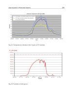
Figure 16 and Figure 17 show the displacement sensor output and the controller output,
respectively, when a step disturbance of 0.05V is applied to the channel 1 input of the
magnetic bearing system when it is controlled with the model based conventional controller
C
lead
(s). Note that the displacement sensor output is multiplied by a factor of 10 when it is
transmitted through the DAC.


Fig. 16. Displacement output of the MBC500 magnetic bearing system with the model based
controller C
lead
(s).


Fig. 17. Control signal of the MBC500 magnetic bearing system with the model based
controller C
lead
(s).

Figure 18 and Figure 19 show the displacement sensor output and the controller output,
respectively, when a step change in disturbance of 0.1V is applied to the channel 1 input of
the magnetic bearing system when it is controlled with the model based controller.


Fig. 18. Step response of the MBC500 magnetic bearing system with the model based
controller C

lead
(s).


Fig. 19. Control signal of the MBC500 magnetic bearing system with the model based
controller C
lead
(s).

Magnetic Bearings, Theory and Applications18

Figure 20 and Figure 21 show the displacement sensor output and the controller output,
respectively, when a step change in disturbance of 0.5V is applied to the channel 1 input of
the magnetic bearing system when it is controlled with the conventional controller C
lead
(s).


Fig. 20. Step response of the MBC500 magnetic bearing system with the model based
controller C
lead
(s).


Fig. 21. Control signal of the MBC500 magnetic bearing system with the model based
controller C
lead
(s).

It can be seen from the above figures that the magnetic bearing system remain stable under

the control of the model based conventional controller when a step change in disturbance of
is applied to its channel 1 input. Similar results were also obtained from other channels.

Figure 22 and Figure 23 show the displacement sensor output and the controller output,
respectively, when a step change in disturbance of 0.05V is applied to the channel 1 input of
the magnetic bearing system when it is controlled with the analytical controller C
2
(s).


Fig. 22. Displacement output of the MBC500 magnetic bearing system with the analytical
controller C
2
(s).


Fig. 23. Control signal of the MBC500 magnetic bearing system with the analytical controller
C
2
(s).
Design and implementation of conventional
and advanced controllers for magnetic bearing system stabilization 19

Figure 20 and Figure 21 show the displacement sensor output and the controller output,
respectively, when a step change in disturbance of 0.5V is applied to the channel 1 input of
the magnetic bearing system when it is controlled with the conventional controller C
lead
(s).

Fig. 20. Step response of the MBC500 magnetic bearing system with the model based
controller C
lead
(s).


Fig. 21. Control signal of the MBC500 magnetic bearing system with the model based
controller C
lead
(s).

It can be seen from the above figures that the magnetic bearing system remain stable under
the control of the model based conventional controller when a step change in disturbance of
is applied to its channel 1 input. Similar results were also obtained from other channels.

Figure 22 and Figure 23 show the displacement sensor output and the controller output,
respectively, when a step change in disturbance of 0.05V is applied to the channel 1 input of
the magnetic bearing system when it is controlled with the analytical controller C
2
(s).


Fig. 22. Displacement output of the MBC500 magnetic bearing system with the analytical
controller C
2
(s).


Fig. 23. Control signal of the MBC500 magnetic bearing system with the analytical controller
C

2
(s).
Magnetic Bearings, Theory and Applications20

Figure 24 and Figure 25 show the displacement sensor output and the controller output,
respectively, when a step change in disturbance of 0.1V is applied to the channel 1 input of
the magnetic bearing system when it is controlled with the analytical controller C
2
(s).


Fig. 24. Displacement output of the MBC500 magnetic bearing system with the analytical
controller C
2
(s).


Fig. 25. Control signal of the MBC500 magnetic bearing system with the analytical controller
C
2
(s).

Figure 26 and Figure 27 show the displacement sensor output and the controller output,
respectively, when a step change in disturbance of 0.5V is applied to the channel 1 input of
the magnetic bearing system when it is controlled with the analytical controller C
2
(s).


Fig. 26. Displacement output of the MBC500 magnetic bearing system with the analytical

controller C
2
(s).


Fig. 27. Control signal of the MBC500 magnetic bearing system with the analytical controller
C
2
(s).

Design and implementation of conventional
and advanced controllers for magnetic bearing system stabilization 21

Figure 24 and Figure 25 show the displacement sensor output and the controller output,
respectively, when a step change in disturbance of 0.1V is applied to the channel 1 input of
the magnetic bearing system when it is controlled with the analytical controller C
2
(s).


Fig. 24. Displacement output of the MBC500 magnetic bearing system with the analytical
controller C
2
(s).


Fig. 25. Control signal of the MBC500 magnetic bearing system with the analytical controller
C
2
(s).

Figure 26 and Figure 27 show the displacement sensor output and the controller output,
respectively, when a step change in disturbance of 0.5V is applied to the channel 1 input of
the magnetic bearing system when it is controlled with the analytical controller C
2
(s).


Fig. 26. Displacement output of the MBC500 magnetic bearing system with the analytical
controller C
2
(s).


Fig. 27. Control signal of the MBC500 magnetic bearing system with the analytical controller
C
2
(s).

Magnetic Bearings, Theory and Applications22

Figure 28 and Figure 29 show the displacement sensor output voltage and the controller
output voltage, respectively, when a step of 0.05V is applied to channel 1 of the magnetic
bearing system, when it is controlled with the FLC.


Fig. 28. Step response of the MBC500 magnetic bearing system with the FLC.


Fig. 29. Control signal of the MBC500 magnetic bearing system with the FLC.

Figure 30 and Figure 31 show the displacement sensor output voltage and the controller
output voltage, respectively, when a step of 0.1V is applied to channel 1 of the magnetic
bearing system, when it is controlled with the FLC.


Fig. 30. Step response of the MBC500 magnetic bearing system with the FLC.


Fig. 31. Control signal of the MBC500 magnetic bearing system with the FLC.
Design and implementation of conventional
and advanced controllers for magnetic bearing system stabilization 23

Figure 28 and Figure 29 show the displacement sensor output voltage and the controller
output voltage, respectively, when a step of 0.05V is applied to channel 1 of the magnetic
bearing system, when it is controlled with the FLC.


Fig. 28. Step response of the MBC500 magnetic bearing system with the FLC.


Fig. 29. Control signal of the MBC500 magnetic bearing system with the FLC.

Figure 30 and Figure 31 show the displacement sensor output voltage and the controller
output voltage, respectively, when a step of 0.1V is applied to channel 1 of the magnetic
bearing system, when it is controlled with the FLC.


Fig. 30. Step response of the MBC500 magnetic bearing system with the FLC.

Fig. 31. Control signal of the MBC500 magnetic bearing system with the FLC.
Magnetic Bearings, Theory and Applications24

Figure 32 and Figure 33 show the displacement sensor output and the controller output,
respectively, when a step change in disturbance of 0.5V is applied to the channel 1 input of
the magnetic bearing system when it is controlled with the FLC.


Fig. 32. Step response of the MBC500 magnetic bearing system with the FLC.


Fig. 33. Control signal of the MBC500 magnetic bearing system with the FLC.

The FLC was tested extensively to ensure that it can operate in a wide range of conditions.
These include testing its tolerance to the resonances of the MBC500 system by tapping the
rotor with screwdrivers. The system remained stable throughout the whole regime of
testing. The MBC500 magnetic bearing system has four different channels; three of the
channels were successfully stabilized with the single FLC designed without any
modifications or further adjustments. For the channel that failed to be robustly stabilized,
the difficulty could be attributed to the strong resonances in that particular channel which
have very large magnitude. After some tuning to the input and output scaling values of the
FLC, robust stabilization was also achieved for this difficult channel.

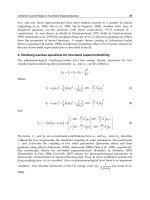
Comparing Figures 16 and 22, 18 and 24, 20 and 26, it can be seen that the system step
responses with the controller designed via analytical interpolation approach exhibit smaller
overshoot and shorter settling time with similar control effort as shown in Figures 17 and 23,
19 and 25, 21 and 27. The step and step disturbance rejection responses with the designed
FLC exhibit smaller steady-state error and overshoot as shown in Figures 28, 30 and 32 with
much bigger control signal displayed in Figures 29, 31 and 33. However, it must be pointed

out that the system stability is achieved with the designed FLC without using the two notch
filters to eliminate the unwanted resonant modes.

9. Conclusion and future work
In this chapter, the controller structure and performance of a conventional controller and an
analytical feedback controller have been compared with those of a fuzzy logic controller
(FLC) when they are applied to the MBC500 magnetic bearing system stabilization problem.

The conventional and the analytical feedback controller were designed on the basis of a
reduced order model obtained from an identified 8
th
-order model of the MBC500 magnetic
bearing system. Since there are resonant modes that can threaten the stability of the closed-
loop system, notch filters were employed to help secure stability.

The FLC uses error and rate of change of error in the position of the rotor as inputs and
produces an output voltage to control the current of the amplifier in the magnetic bearing
system. Since a model is not required in this approach, this greatly simplified the design
process. In addition, the FLC can stabilize the magnetic bearing system without the use of
any notch filters. Despite the simplicity of FLC, experimental results have shown that it
produces less steady-state error and has less overshoot than its model based counterpart.

While the model based controllers are linear systems, it is not a surprise that their stability
condition depends on the level of the disturbance. This is because the magnetic bearing
system is a nonlinear system. However, although the FLC exhibits some of the common
characteristics of high authority linear controllers (small steady-state error and amplification
of measurement noise), it does not have the low stability robustness property usually
associated with such high gain controllers that we would have expected.

Future work will include finding some explanations for the above unusual observation on

FLC. We believe the understanding achieved through attempting to address the above issue
would lead to better controller design methods for active magnetic bearing systems.
Design and implementation of conventional
and advanced controllers for magnetic bearing system stabilization 25

Figure 32 and Figure 33 show the displacement sensor output and the controller output,
respectively, when a step change in disturbance of 0.5V is applied to the channel 1 input of
the magnetic bearing system when it is controlled with the FLC.


Fig. 32. Step response of the MBC500 magnetic bearing system with the FLC.


Fig. 33. Control signal of the MBC500 magnetic bearing system with the FLC.

The FLC was tested extensively to ensure that it can operate in a wide range of conditions.
These include testing its tolerance to the resonances of the MBC500 system by tapping the
rotor with screwdrivers. The system remained stable throughout the whole regime of
testing. The MBC500 magnetic bearing system has four different channels; three of the
channels were successfully stabilized with the single FLC designed without any
modifications or further adjustments. For the channel that failed to be robustly stabilized,
the difficulty could be attributed to the strong resonances in that particular channel which
have very large magnitude. After some tuning to the input and output scaling values of the
FLC, robust stabilization was also achieved for this difficult channel.

Comparing Figures 16 and 22, 18 and 24, 20 and 26, it can be seen that the system step
responses with the controller designed via analytical interpolation approach exhibit smaller
overshoot and shorter settling time with similar control effort as shown in Figures 17 and 23,
19 and 25, 21 and 27. The step and step disturbance rejection responses with the designed
FLC exhibit smaller steady-state error and overshoot as shown in Figures 28, 30 and 32 with

much bigger control signal displayed in Figures 29, 31 and 33. However, it must be pointed
out that the system stability is achieved with the designed FLC without using the two notch
filters to eliminate the unwanted resonant modes.

9. Conclusion and future work
In this chapter, the controller structure and performance of a conventional controller and an
analytical feedback controller have been compared with those of a fuzzy logic controller
(FLC) when they are applied to the MBC500 magnetic bearing system stabilization problem.

The conventional and the analytical feedback controller were designed on the basis of a
reduced order model obtained from an identified 8
th
-order model of the MBC500 magnetic
bearing system. Since there are resonant modes that can threaten the stability of the closed-
loop system, notch filters were employed to help secure stability.

The FLC uses error and rate of change of error in the position of the rotor as inputs and
produces an output voltage to control the current of the amplifier in the magnetic bearing
system. Since a model is not required in this approach, this greatly simplified the design
process. In addition, the FLC can stabilize the magnetic bearing system without the use of
any notch filters. Despite the simplicity of FLC, experimental results have shown that it
produces less steady-state error and has less overshoot than its model based counterpart.

While the model based controllers are linear systems, it is not a surprise that their stability
condition depends on the level of the disturbance. This is because the magnetic bearing
system is a nonlinear system. However, although the FLC exhibits some of the common
characteristics of high authority linear controllers (small steady-state error and amplification
of measurement noise), it does not have the low stability robustness property usually
associated with such high gain controllers that we would have expected.

Future work will include finding some explanations for the above unusual observation on
FLC. We believe the understanding achieved through attempting to address the above issue
would lead to better controller design methods for active magnetic bearing systems.
Magnetic Bearings, Theory and Applications26

10. References
Williams, R.D, Keith, F.J., and Allaire, P.E. (1990). Digital Control of Active Magnetic
Bearing, IEEE trans. on Indus. Electr. Vol. 37, No. 1, pp. 19-27, February 1990.
Lee, K.C, Jeong, Y.H., Koo, D.H., and Ahn, H. (2006) Development of a Radial Active
Magnetic Bearing for High Speed Turbo-machinery Motors, Proceedings of the 2006
SICE-ICASE International Joint Conference, 1543-1548, 18-21 October, 2006.
Bleuler, H., Gahler, C., Herzog, R., Larsonneur, R., Mizuno, T., Siegwart, R. (1994)
Application of Digital Signal Processors for Industrial Magnetic Bearings, IEEE
Trans. on Control System Technology, Vol. 2, No. 4, pp. 280-289, December 1994.
Magnetic Moments (1995), LLC, MBC 500 Magnetic Bearing System Operating Instructions,
December, 1995.
Shi, J. and Revell, J. (2002) System Identification and Reengineering Controllers for a
Magnetic Bearing System, Proceedings of the IEEE Region 10 Technical Conference on
Computer, Communications, Control and Power Engineering, Beijing, China, pp.1591-
1594, 28-31 October, 2002.
Dorato, P. (1999) Analytic Feedback System Design: An Interpolation Approach, Brooks/Cole,
Thomson Learning, 1999.
Dorato, P., Park, H.B., and Li, Y. (1989) An Algorithm for Interpolation with Units in H∞,
with Applications to Feedback Stabilization, Automatica, Vol. 25, pp.427-430, 1989.
Shi, J., and Lee, W.S. (2009) Analytical Feedback Design via Interpolation Approach for the
Strong Stabilization of a Magnetic Bearing System, Proceedings of the 2009 Chinese
Control and Decision Conference (CCDC2009), Guilin, China, 17-19 June, 2009, pp.
280-285.
Shi, J., Lee, W.S., and Vrettakis, P. (2008) Fuzzy Logic Control of a Magnetic Bearing System,
Proceedings of the 20th Chinese Control and Decision Conference(2008 CCDC), Yantai,

China, 1-6, 2-4 July, 2008.
Shi, J., and Lee, W.S. (2009) An Experimental Comparison of a Model Based Controller and a
Fuzzy Logic Controller for Magnetic Bearing System Stabilization, Proceedings of the
7
th
IEEE International Conference on Control & Automation (ICCA’09), Christchurch,
New Zealand, 9-11 December, 2009, pp. 379-384.
Habib, M.K., and Inayat-Hussain, J.I. (2003). Control of Dual Acting Magnetic Bearing
Actuator System Using Fuzzy Logic, Proceedings 2003 IEEE International Symposium
on Computational Intelligence in Robotics and Automation, Kobe, Japan, pp. 97-101, July
16-20, 2003.
Morse, N., Smith, R. and Paden, B. (1996) Magnetic Bearing System Identification, MBC 500
Magnetic System Operating Instructions, pp.1-14, May 29, 1996.
Van den Hof, P.M.J. and Schrama, R.J.P. (1993) “An indirect method for transfer function
estimation from closed-loop data”, Automatica, Volume 29, Issue 6, pp.1523-1527,
1993.
Freudenberg, J.S. and Looze, D.P. (1985), Right Half Plane Poles and Zeros and Design
Tradeoffs in Feedback Systems, IEEE Trans. Automat. Control, 30, pp.555-565, 1985.
Dorato, P. (1999) Analytic Feedback System Design: An Interpolation Approach, Brooks/Cole,
Thomson Learning, 1999.
Youla, D.C., Borgiorno J.J. Jr., and Lu, C.N. (1974) Single-loop feedback stabilization of linera
multivariable dynamical plants, Automatica, Vol. 10, 159-173, 1974.
Passino, K.M. and Yurkovich, S. (1998) Fuzzy Control, Addison-Wesley Longman, Inc., 1998.
Linearization of radial force characteristic
of active magnetic bearings using nite element method and differential evolution 27
Linearization of radial force characteristic of active magnetic bearings
using nite element method and differential evolution
Boštjan Polajžer, Gorazd Štumberger, Jože Ritonja and Drago Dolinar
X

Linearization of radial force characteristic of
active magnetic bearings using finite element
method and differential evolution

Boštjan Polajžer, Gorazd Štumberger, Jože Ritonja and Drago Dolinar
University of Maribor, Faculty of Electrical Engineering and Computer Science
Slovenia

1. Introduction

Active magnetic bearings (AMBs) are used to provide contact-less suspension of a rotor
(Schweitzer et al., 1994). No friction, no lubrication, precise position control, and vibration
damping make AMBs appropriate for different applications. In-depth debate about the
research and development has been taken place the last two decades throughout the
magnetic bearings community (ISMB12, 2010). However, in the future it is likely to be
focused towards the superconducting applications of magnetic bearings (Rosner, 2001).
Nevertheless, the discussion in this work is restricted to the design and analysis of
“classical” AMBs, which are indispensable elements for high-speed, high-precision machine
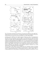
tools (Larsonneur, 1994). Two radial AMBs, which control the vertical and horizontal rotor
displacements in four degrees of freedom (DOFs) are placed at the each end of the rotor,
whereas an axial AMB is used to control the fifth DOF, as it is shown in Fig. 1. Rotation (the
sixth DOF) is controlled by an independent driving motor. Because AMBs constitute an
inherently unstable system, a closed-loop control is required to stabilize the rotor position.
Different control techniques (Knospe & Collins, 1996) are employed to achieve advanced
features of AMB systems, such as higher operating speeds or control of the unbalance
response. However, a decentralized PID feedback is, even nowadays, normally used in
AMB industrial applications, whereas prior to a decade ago, more than 90% of the AMB
systems were based on PID decentralized control (Bleuer et al., 1994).

Fig. 1. Typical AMB system
2
Magnetic Bearings, Theory and Applications28

The development and design of AMBs is a complex process, where possible
interdependencies of requirements and constrains should be considered. This can be done
either by trials using analytical approach (Maslen, 1997), or by applying numerical
optimization methods (Meeker, 1996; Carlson-Skalak et al., 1999; Štumberger et al., 2000).
AMBs are a typical non-linear electro-magneto-mechanical coupled system. A combination
of stochastic search methods and analysis based on the finite element method (FEM) is
recommended for the optimization of such constrained, non-linear electromagnetic systems
(Hameyer & Belmans, 1999).
In this work the numerical optimization of radial AMBs is performed using differential
evolution (DE) – a direct search algorithm (Price et al., 2005) – and the FEM (Pahner et al.,
1998). The objective of the optimization is to linearize current and position dependent radial
force characteristic over the entire operating range. The objective function is evaluated by
two dimensional FEM-based magnetostatic computations, whereas the radial force is
determined using Maxwell’s stress tensor method. Furthermore, through the comparison of
the non-optimized and optimized radial AMB, the impact of non-linearities of the radial
force characteristic, on static and dynamic properties of the overall system is evaluated over
the entire operating range.

2. Radial Force Characteristic of Active Magnetic Bearings

An eight-pole radial AMB is discussed, as it is shown in Fig. 2. The windings of all
electromagnets are supplied in such a way, that a NS-SN-NS-SN pole arrangement is
achieved. Four independent magnetic circuits – electromagnets are obtained in such way.
The electromagnets in the same axis generate the attraction forces acting on the rotor in
opposite directions. The resultant radial force of such a pair of electromagnets is a non-linear
function of the currents, rotor position, and magnetization of the iron core. The differential

driving mode of currents is introduced by the following definitions: i
1
= I
0
+ i
x
, i
2
= I
0
 i
x
,
i
3
= I
0
+ i
y
, and i
4
= I
0
 i
y
, where I
0
is the constant bias current, i
x
and i

y
are the control
currents in the x and y axis, where | i
x
| ≤ I
0
, and | i
y
| ≤ I
0
.


Fig. 2. Eight-pole radial AMB

2.1 Linearized AMB model for one axis
When the magnetic non-linearities and cross-coupling effects are neglected, the force
generated by a pair of electromagnets in the x axis can be expressed by (1).

0
is the nominal
air gap for the rotor central position (x = y = 0),

0
is permeability of vacuum, N is the
number of turns of each coil, and A is the area of one pole. Note that the force generated by
a pair of electromagnets in the y axis is defined in the same way as in (1).

 
2 2

2
0 0
0
0 0
1
cos 8
4
x x
x
I i I i
F AN
x x
 
 
 
   
 
 
 
   
 
 
   
 

(1)

Non-linear equation (1) can be linearized at a nominal operating point (x = 0, i
x
= 0). The

obtained linear equation (2) is valid only in the vicinity of the point of linearization. In such
way two parameters are introduced at a nominal operating point; the current gain h
x,nom

by (3) and the position stiffness c
x,nom
by (4).

,nom ,nomx x x x
F h i c x



(2)
 
2
0
,nom 0
2
0
( 0, 0)
cos 8
x
x
x
x
i x
F I
h AN
i

 

 

 


(3)
 
2
2
0
,nom 0
3
0
( 0, 0)
cos 8
x
x
x
i x
F I
c AN
x
 

 

 


(4)

The motion of the rotor between two electromagnets in the x axis is described by (5), where
m is the mass of the rotor. When the equation (2) is used then the linearized AMB model for
one axis is described by (6).
2
2
x
d x
F m
dt


(5)
2
,nom ,nom
2
x x
x
h c
d x
i x
dt m m
 

(6)

The dynamic model (6) is used for determining the controller settings, where the nominal
values of the model parameters are used (h

x,nom
and c
y,nom
). However, due to the magnetic
non-linearities, the current gain and position stiffness vary according to the operating point.
Consequently, a damping and stiffness of the closed-loop system might be deteriorated in
the cases of high signal amplitudes, such as heavy load unbalanced operation.

2.2 Magnetic field distribution and radial force computation using FEM
The magnetostatic problem is formulated by Poisson's equation (7), where A denotes the
magnetic vector potential,

is the magnetic reluctivity, J is the current density,  denotes the
dot product and  is the Hamilton's differential operator.





   A J

(7)