An Introduction to Financial Option Valuation_9 doc

19.7 Notes and references 197
Chapter 13 of (Bj
¨
ork, 1998) deals with barriers and lookbacks from a
martingale/risk-neutral perspective.
The use of the binomial method for barriers, lookbacks and Asians is discussed
in (Hull, 2000; Kwok, 1998).
There are many ways in which the features discussed in this chapter have been
extended and combined to produce ever more exotic varieties. In particular, early
exercise can be built into almost any option. Examples can be found in (Hull,
2000; Kwok, 1998; Taleb, 1997; Wilmott, 1998).
Practical issues in the use of the Monte Carlo and binomial methods for exotic
options are treated in (Clewlow and Strickland, 1998).
From a trader’s perspective, ‘how to hedge’ is more important than ‘how to
value’. The hedging issue is covered in (Taleb, 1997; Wilmott, 1998).
EXERCISES
19.1.  Suppose that the function V (S, t) satisfies the Black–Scholes PDE
(8.15). Let

V (S, t) := S
1−
2r
σ
2
V

X
S
, t

.

Show that
∂

V
∂t
+
1
2
σ
2
S
2
∂
2

V
∂ S
2
+rS
∂

V
∂ S
−r

V = S
1−
2r
σ
2


∂V
∂t

X
S
, t

+
1
2
σ
2

X
S

2
∂
2
V
∂ S
2

X
S
, t

+r
X

S
∂V
∂ S

X
S
, t

−rV

X
S
, t


.
Deduce that

V (S, t) solves the Black–Scholes PDE.
19.2.  Using Exercise 19.1, deduce that C
B
in (19.3) satisfies the Black–
Scholes PDE (8.15). Confirm also that C
B
satisfies the conditions (19.1)
and (19.2) when B < E.
19.3.  Explain why (19.4) holds for all ‘down’ and ‘up’ barrier options.
19.4.  Why does it not make sense to have B < E in an up-and-in call option?
19.5.  The value of an up-and-out call option should approach zero as S ap-
proaches the barrier B from below. Verify that setting S = B in (19.5) re-

turns the value zero.
19.6. Consider the geometric average price Asian call option, with payoff
max



n

i=1
S(t
i
)

1/n
− E, 0


,
198 Exotic options
where the points {t
i
}
n
i=1
are equally spaced with t
i
= it and nt = T .
By writing
n


i=1
S(t
i
) =
S(t
n
)
S(t
n−1
)

S(t
n−1
)
S(t
n−2
)

2

S(t
n−2
)
S(t
n−3
)

3
···


S(t
3
)
S(t
2
)

n−2

S(t
2
)
S(t
1
)

n−1

S(t
1
)
S
0

n
S
n
0
and using the ‘additive mean and variance’ property of independent normal
random variables mentioned as item (iii) at the end of Section 3.5, show

that for the asset model (6.9) under risk neutrality, we have
log



n

i=1
S(t
i
)

1/n

S
0


= N

(r −
1
2
σ
2
)
(n +1)
2n
T,σ
2

(n +1)(2n +1)
6n
2
T

.
(Note in particular that this establishes a lognormality structure, akin to that
of the underlying asset.) Valuing the option as the risk-neutral discounted
expected payoff, deduce that the time-zero option value is equivalent to
the discounted expected payoff for a European call option whose asset has
volatility σ satisfying
σ
2
= σ
2
(n + 1)(2n + 1)
6n
2
and drift µ given by
µ =
1
2
σ
2
+ (r −
1
2
σ
2
)

(n + 1)
2n
.
Use Exercise 12.4 and the Black–Scholes formula (8.19) to deduce that the
time-zero geometric average price Asian call option value can be written
e
−rT

S
0
e
µT
N (

d
1
) − EN(

d
2
)

, (19.10)
where

d
1
=
log(S
0

/E) + (µ +
1
2
σ
2
)T
σ
√
T
,

d
2
=

d
1
−σ
√
T .
19.8 Program of Chapter 19 and walkthrough 199
19.7.  Write down a pseudo-code algorithm for Monte Carlo applied to a float-
ing strike lookback put option.
19.8 Program of Chapter 19 and walkthrough
In ch19, listed in Figure 19.4, we value an up-and-out call option. The first part of the code is a
straightforward evaluation of the Black–Scholes formula (19.5). The second part shows how a Monte
Carlo approach can be used. This code follows closely the algorithm outlined in Section 19.6, except
that the asset path computation is vectorized: rather than loop for j=0:N-1,wecompute the
full path in one fell swoop, using the cumprod function that we encountered in ch07.
Running ch19 gives bsval = 0.1857 for the Black–Scholes value and conf = [0.1763,

0.1937] for the Monte Carlo confidence interval.
PROGRAMMING EXERCISES
P19.1. Use a Monte Carlo approach to value a floating strike lookback put option.
P19.2. Implement the binomial method for a shout option, using (19.9), and in-
vestigate its rate of convergence.
Quotes
There are so many of them, and some of them are so esoteric,
that the risks involved may not be properly understood
even by the most sophisticated of investors.
Some of these instruments appear to be specifically designed to enable institutions
to take gambles which they would otherwise not be permitted to take . . .
One of the driving forces behind the development of derivatives
wastoescape regulations.
GEORGE SOROS, source (Bass, 1999)
The standard theory of contingent claim pricing through dynamic replication
gives no special role to options.
Using Monte Carlo simulation, path-dependent multivariate claims of great complexity
can be priced as easily as the path-independent univariate hockey-stick payoffs which
characterize options.
It is thus not at all obvious why markets have organized to offer these simple payoffs,
when other collections of functions
such as polynomials, circular functions, or wavelets
might offer greater advantages.
PETER CARR, KEITH LEWIS AND DILIP MADAN, ‘On The Nature of Options’,
Robert H. Smith School of Business, Smith Papers Online, 2001, source
/>Do you believe that huge losses on derivatives are confined to reckless or dim-witted
institutions?
200 Exotic options
%CH19 Program for Chapter 19
%

% Up-and-out call option
% Evaluates Black-Scholes formula and also uses Monte Carlo
randn(’state’,100)
%%%%%%%%% Problem and method parameters %%%%%%%%%%%
S=5;E=6;sigma = 0.25;r=0.05;T=1;B=9;
Dt = 1e-3;N=T/Dt;M=1e4;
%%%%%%%%%%%%%%%%%%%%%%%%%%%%%%%%%%%%%%
%%%%%%%%%%%%%%% Black-Scholes value %%%%%%%%%%%%%%%
tau=T;
power1 = -1 + (2*r)/(sigmaˆ2);
power2 =1+(2*r)/(sigmaˆ2);
d1 = (log(S/E) + (r + 0.5*sigmaˆ2)*(tau))/(sigma*sqrt(tau));
d2 = d1 - sigma*sqrt(tau);
e1 = (log(S/B) + (r + 0.5*sigmaˆ2)*(tau))/(sigma*sqrt(tau));
e2 = (log(S/B) + (r - 0.5*sigmaˆ2)*(tau))/(sigma*sqrt(tau));
f1 = (log(S/B) - (r - 0.5*sigmaˆ2)*(tau))/(sigma*sqrt(tau));
f2 = (log(S/B) - (r + 0.5*sigmaˆ2)*(tau))/(sigma*sqrt(tau));
g1 = (log(S*E/(Bˆ2)) - (r - 0.5*sigmaˆ2)*(tau))/(sigma*sqrt(tau));
g2 = (log(S*E/(Bˆ2)) - (r + 0.5*sigmaˆ2)*(tau))/(sigma*sqrt(tau));
Nd1 = 0.5*(1+erf(d1/sqrt(2))); Nd2 = 0.5*(1+erf(d2/sqrt(2)));
Ne1 = 0.5*(1+erf(e1/sqrt(2))); Ne2 = 0.5*(1+erf(e2/sqrt(2)));
Nf1 = 0.5*(1+erf(f1/sqrt(2))); Nf2 = 0.5*(1+erf(f2/sqrt(2)));
Ng1 = 0.5*(1+erf(g1/sqrt(2))); Ng2 = 0.5*(1+erf(g2/sqrt(2)));
a=(B/S)ˆpower1; b = (B/S)ˆpower2;
bsval = S*(Nd1-Ne1-b*(Nf2-Ng2)) - E*exp(-r*tau)*(Nd2-Ne2-a*(Nf1-Ng1))
%%%%%%%%%%%%%%%%%%%%%%%%%%%%%%%%%%%%%%%
V=zeros(M,1);
for i = 1:M
Svals = S*cumprod(exp((r-0.5*sigmaˆ2)*Dt+sigma*sqrt(Dt)*randn(N,1)));
Smax = max(Svals);

if Smax < B
V(i) = exp(-r*T)*max(Svals(end)-E,0);
end
end
aM = mean(V); bM = std(V);
conf = [aM - 1.96*bM/sqrt(M), aM + 1.96*bM/sqrt(M)]
Fig. 19.4. Program of Chapter 19: ch19.m.
19.8 Program of Chapter 19 and walkthrough 201
If so, consider:
Procter & Gamble (lost $102 million in 1994)
Gibson Greetings (lost $23 million in 1994)
Orange County, California (bankrupted after $1.7 billion loss in 1994)
Baring’s Bank (bankrupted after $1.3 billion loss in 1995)
Sumitomo (lost $1.3 billion in 1996)
Government of Belgium ($1.2 billion loss in 1997)
National Westminster Bank (lost $143 million in 1997)
PHILIP MCBRIDE JOHNSON (Johnson, 1999)

20
Historical volatility
OUTLINE
• Monte Carlo type estimates
• maximum likelihood estimates
• exponentially weighted moving averages
20.1 Motivation
We know that the volatility parameter, σ ,inthe Black–Scholes formula cannot be
observed directly. In Chapter 14 we saw how σ for a particular asset can be esti-
mated as the implied volatility, based on a reported option value. In this chapter
we discuss another widely used approach – estimating the volatility from the pre-
vious behaviour of the asset. This technique is independent of the option valuation

problem. Here is the basic principle.
Given that we have (a) a model for the behaviour of the asset price that involves σ and (b)
access to asset prices for all times up to the present, let us fit σ in the model to the observed
data.
Avalue σ

arising from this general procedure is called a historical volatility
estimate.
20.2 Monte Carlo type estimates
We suppose that historical asset price data is available at equally spaced time val-
ues t
i
:= it,soS(t
i
) is the asset price at time t
i
.Wethen define the log ratios
U
i
:= log
S(t
i
)
S(t
i−1
)
. (20.1)
Our asset price model (6.9) assumes that the {U
i
} are independent, normal ran-

dom variables with mean (µ −
1
2
σ
2
)t and variance σ
2
t. From this point of
view, getting hold of historical asset price data and forming the log ratios is
203
204 Historical volatility
equivalent to sampling from an N((µ −
1
2
σ
2
)t,σ
2
t) distribution. Hence, we
could use a Monte Carlo approach to estimate the mean and variance. Sup-
pose that t = t
n
is the current time and that the M + 1 most current asset prices
{S(t
n−M
), S(t
n−M+1
), ,S(t
n−1
), S(t

n
)} are available. Using the corresponding
log ratio data, {U
n+1−i
}
M
i=1
, the sample mean (15.1) and variance estimate (15.2)
become
a
M
:=
1
M
M

i=1
U
n+1−i
, (20.2)
b
2
M
:=
1
M − 1
M

i=1
(U

n+1−i
− a
M
)
2
. (20.3)
We may therefore estimate the unknown parameter σ by comparing the sample
mean a
M
with the exact mean (µ −
1
2
σ
2
)t from the model, or by comparing the
sample variance b
2
M
with the exact variance σ
2
t from the model. In practice the
latter works much better – see Exercise 20.1 – and hence we let
σ

:=
b
M
√
t
. (20.4)

Exercise 20.2 shows that this can be written directly in terms of the U
i
values as
σ

=





1
t


1
M − 1
M

i=1
U
2
n+1−i
−
1
M(M − 1)

M

i=1

U
n+1−i

2


. (20.5)
20.3 Accuracy of the sample variance estimate
To get some idea of the accuracy of the estimate σ

in (20.4) we take the view
that we are essentially using Monte Carlo simulation to compute b
2
M
as an approx-
imation to the expected value of the random variable (U −
E(U))
2
, where U ∼
N((µ −
1
2
σ
2
)t,σ
2
t). (This is not exactly the case, as we are using an approxi-
mation to
E(U).) Equivalently, after dividing through by t,weare using Monte
Carlo simulation to compute σ


2
= b
2
M
/t as an approximation to the expected
value of the random variable


U −
E


U

2
, where

U ∼ N((µ −
1
2
σ
2
)
√
t,σ
2
).
Hence, from (15.5), an approximate 95% confidence interval for σ
2

is given by
σ

2
±
1.96v
√
M
,
where v
2
is the variance of the random variable


U − E


U

2
.Exercise 20.3 shows
that
v
2
= 2σ
4
. (20.6)
20.3 Accuracy of the sample variance estimate 205
So the approximate confidence interval for σ
2

has the form
σ

2
±
1.96
√
2σ
2
√
M
. (20.7)
It may then be argued that
σ

±
1.96σ

√
2M
(20.8)
is an approximate 95% confidence interval for σ ,see Exercise 20.4. In particular,
we recover the usual 1/
√
M behaviour.
There is, however, a subtle point to be made. In a typical Monte Carlo simula-
tion, taking more samples (increasing M) means making more calls to a pseudo-
random number generator. In the above context, though, taking more samples
means looking up more data. There are two natural ways to do this.
(1) Keep t fixed and simply go back further in time.

(2) Fix the time interval, Mt, over which the data is sampled and decrease t.
Both approaches are far from perfect. Case (1) runs counter to the intuitive notion
that recent data is more important than old data. (The asset price yesterday is more
relevant than the asset price last year.) We will return to this issue later. Case (2)
suffers from a practical limitation: the bid–ask spread introduces a noisy compo-
nent into the asset price data that becomes significant when very small t values
are measured. Overall, finding a compromise between large M and small t is a
difficult task.
If σ

is computed in order to value an option, then a widely quoted rule of
thumb is to make the historical data time-frame Mt equal to that of the option:
to value an option that expires in six months’ time, take six months of histori-
cal data. There is also some evidence that taking longer historical data periods is
worthwhile.
Using the identity log(a/b) = log a − log b to simplify (20.2) we find that
a
M
=
1
M
M

i=1
(
log S(t
n+1−i
) − log S(t
n−i
)

)
=
1
M
(
log S(t
n
) − log S(t
n−M
)
)
=
1
M
log
S(t
n
)
S(t
n−M
)
.
Because those intermediate terms cancel, a
M
depends only on the first and last
S values! Our asset price model assumes that log(S(t
n
)/S(t
n−M
)) is normal with

206 Historical volatility
mean (µ −
1
2
σ
2
)Mt and variance σ
2
Mt. Hence,
a
M
∼ N

(µ −
1
2
σ
2
)t,σ
2
t
M

. (20.9)
In practice, because a
M
is normal with small mean and variance, it is common to
replace it by zero in (20.3), which leads to
σ


=




1
t
1
(M − 1)
M

i=1
U
2
n+1−i
, (20.10)
instead of (20.5). This alternative has been found to be more reliable in general.
20.4 Maximum likelihood estimate
To justify further the historical volatility estimate (20.10), we will show that an
almost identical quantity
σ

=




1
t
1

M
M

i=1
U
2
n+1−i
(20.11)
can be derived from a maximum likelihood viewpoint. Note that (20.11) differs
from (20.10) only in that M − 1 has become M.
The maximum likelihood principle is based on the following idea:
In the absence of any extra information, assume the event that we observed was the one
that was most likely to happen.
In terms of fitting an unknown parameter, the idea becomes:
Choose the parameter value that makes the event that we observed have the maximum
probability.
As a simple example, consider the case where a coin is flipped four times.
Suppose we think the coin is potentially biased – there is some p ∈ [0, 1] such
that, independently on each flip, the probability of heads (H) is p and the proba-
bility of tails (T) is 1 − p. Suppose the four flips produce H,T,T,H. Then, under
our assumption, the probability of this outcome is p × (1 − p) × (1 − p) × p =
p
2
(1 − p)
2
. Simple calculus shows that maximizing p
2
(1 − p)
2
over p ∈ [0, 1]

leads to p =
1
2
, which is, of course, intuitively reasonable for that data. Similarly,
if we observed H,T,H,H, the resulting probability is p
3
(1 − p).Inthis case, max-
imizing over p ∈ [0, 1] gives p =
3
4
, also agreeing with our intuition.
That simple example involved a sequence of independent observations, where
each observation (the result of a coin flip) is a discrete random variable. In the
20.5 Other volatility estimates 207
case where the model involves outcomes, say U
1
, U
2
, ,U
M
, from a continuous
random variable with density f (x) that involves some parameter, we look for the
parameter value that maximizes the product
f (U
1
) f (U
2
) f (U
M
).

Formally, this maximizes the value of the corresponding probability density func-
tion at the point (U
1
, U
2
, ,U
M
).
Returning to the case of estimating the value σ from our observations of U
i
in (20.1), we first make a simplification. On the basis that U
i
/
√
t ∼ N((µ −
1
2
σ
2
)
√
t,σ
2
),wetake the view that the mean of U
i
/
√
t is negligible, and re-
gard it as zero. The corresponding density function for each scaled observation
U

i
/
√
t becomes
f (x) =
1
√
2πσ
2
e
−x
2
/(2σ
2
)
.
Our maximum likelihood estimate of σ is then found by maximizing
M

i=1
1
√
2πσ
2
e
−

U
2
n+1−i

/(2σ
2
)
, where

U
n+1−i
= U
√
t
n+1−i
(20.12)
Exercise 20.5 shows that this leads to the estimate (20.11).
20.5 Other volatility estimates
Under the simplifying assumption that U
i
has zero mean, var(U
i
) = E(U
2
i
).For
the estimate (20.11) we have
tσ

2
=
1
M
M


i=1
U
2
n+1−i
,
and hence we may interpret tσ

2
as a sample mean approximation for this ex-
pected value. Keep in mind that the samples, U
2
i
, correspond to different points
in time. It has been found that rather than treating each observation U
i
equally it
is more appropriate to give extra weight to the most recent values. This leads to
schemes of the general form
tσ

2
=
M

i=1
α
i
U
2

n+1−i
, where
M

i=1
α
i
= 1, (20.13)
208 Historical volatility
with α
1
>α
2
> ···>α
M
> 0. It is common to use geometrically declining
weights: α
i+1
= wα
i
, for some 0 <w<1. This produces the estimate
tσ

2
=

M
i=1
w
i

U
2
n+1−i

M
i=1
w
i
.
The choice w = 0.94 is popular. Note that (0.94)
10
≈ 0.54, (0.94)
100
≈ 0.0021
and (0.94)
200
< 10
−5
,sointhis case, even if M is chosen to be very large, samples
more than around a hundred t units old are essentially ignored.
If a new volatility estimate is needed at each time t
n
, there is a neat variation of
this idea. Suppose tσ

n
2
is our estimate of tσ
2
computed at time t

n
, based on
{U
n+1−i
}
M
i=1
. Then an estimate for time t
n+1
can be computed as
tσ

n+1
2
= wtσ

n
2
+ (1 − w)U
2
n+1
. (20.14)
This process is close to having geometrically declining weights, see Exercise 20.7,
and has the advantage that updating from time t
n
to time t
n+1
does not require the
old data U
i

, for i ≤ n,tobeaccessed.
Formulas such as (20.14) are sometimes referred to as exponentially weighted
moving average (EWMA) models. Of course, the notion of computing a time-
varying estimate of the volatility is inherently at odds with the underlying assump-
tion of constant volatility that is used in the derivation of the Black–Scholes for-
mula. Even so, it has been observed empirically that asset price volatility is not
constant, and techniques that account for this fact have proved successful.
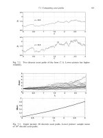
20.6 Example with real data
In Figure 20.1 we estimate historical volatility for the IBM daily and weekly data
from Figures 5.1 and 5.2. In both cases, we assume that the data corresponds to
equally spaced points in time. The daily data runs over 9 months (T = 3/4 years)
and has 183 asset prices (M = 182), so we set t = T/M ≈ 0.0041. The weekly
data runs over 4 years (T = 4) and has 209 asset prices (M = 208), so we set
t = T/M ≈ 0.0192.
For the daily data we found a
M
=−4.3 × 10
−4
, confirming that it is reason-
able to regard the log ratio mean as zero. The Monte Carlo based estimate (20.4)
produced σ

= 0.4069 with a 95% confidence interval of [0.3653, 0.4486]. Given
that a
M
≈ 0, it is not surprising that the simpler estimate (20.10) produced an
almost identical value σ

= 0.4070. This σ


is represented as a dashed line in
the upper picture. The EWMA is plotted as diamond shaped markers joined by
straight lines. Here, we used the first 20 U
i
values to compute a Monte Carlo based
estimate, and inserted this as a starting value for σ

in the update formula (20.14).
Our weight was w = 0.94.
20.7 Notes and references 209
20 40 60 80 100 120 140 160 180
0
0.2
0.4
0.6
0.8
1
Days
Vol
Daily
20 40 60 80 100 120 140 160 180 200
0
0.2
0.4
0.6
0.8
1
Weeks
Vol
Weekly

Fig. 20.1. Historical volatility estimates for IBM data from Figures 5.1 and
5.2. Upper picture: daily. Lower picture: weekly. Diamonds are exponentially
weighted moving averages. Dashed lines show the estimate (20.10).
The lower picture repeats the exercise for the weekly data. In this case (20.4)
produced σ

= 0.3610 with a 95% confidence interval of [0.3263, 0.3957]. We
found that a
M
=−4.0 × 10
−3
and the estimate (20.10) gave σ

= 0.3621.
Overall, the small size of the sample mean a
M
and the reasonable agreement
between the daily and weekly σ

estimates are encouraging. However, the large
confidence intervals for these estimates, and the significant time dependency of
the EWMA, are far from reassuring. Generally, extracting historical volatility es-
timates from real data is a mixture of art and science.
20.7 Notes and references
Volatility estimation is undoubtedly one of the most important aspects of practical
option valuation, and it remains an active research topic, see (Poon and Granger,
2003), for example.
More sophisticated time-varying volatility models, including autoregressive
conditional heteroscedasticity (ARCH) and generalized autoregressive conditional
heteroscedasticity (GARCH) are discussed in (Hull, 2000), for example.

In addition to providing information for option valuation, historical volatility
estimates are a key component in the determination of Value at Risk; see (Hull,
2000, Chapter 4), for example.
210 Historical volatility
EXERCISES
20.1.  Consider a Monte Carlo approach where the sample mean a
M
in
(20.2) is used to approximate the exact mean (µ −
1
2
σ
2
)t in order to es-
timate σ . Suppose that a fixed time-frame Mt is used for the log ratios.
This corresponds to case (2) in Section 20.3. Show that the 95% confidence
interval for the mean has width proportional to 1/M. Convince yourself that
this is a poor method. [Hint: use (20.9) and refer to Chapter 15.]
20.2.  Establish (20.5).
20.3.  Let Z ∼ N(0, 1) and Y = α + β Z, for α, β ∈
R. Show that
var

(Y −
E(Y))
2

= 2β
4
. Hence, verify (20.6).

20.4.  Use the expansion
√
1 ±  ≈ 1 ±
1
2
 for small >0, to show how the
approximate confidence interval (20.8) may be inferred from (20.7).
20.5. Show that maximizing (20.12) with respect to σ leads to the estimate
(20.11). [Hints: (1) take logs – maximizing a positive quantity is equivalent
to maximizing its log, (2) regard σ
2
as the unknown parameter, rather than
σ .]
20.6.  Give a convincing argument for the constraint

M
i=1
α
i
= 1in(20.13).
20.7.  Explain why (20.14) almost corresponds to having geometrically declin-
ing weights.
20.8 Program of Chapter 20 and walkthrough
In ch20, listed in Figure 20.2, we look at historical volatility estimation with artificial data, cre-
ated with a random number generator. The array U has ith entry given by the log of the ratio
asset(i+1)/asset(i), where the asset path, asset,iscreated in the usual way, using a volatility
of sigma = 0.3. The Monte Carlo volatility estimate (20.4) turns out to be 0.2947, with an ap-
proximate confidence interval (20.8) of cont = [0.2855, 0.3038]. The simplified estimate with
sample mean set to zero also gives sigma2 = 0.2947.Wethen apply the EWMA formula (20.14)
with w = 0.94, using a Monte Carlo estimate of the first twenty U values to initialize the volatility.

The running estimate, s,isplotted and the exact level 0.3issuperimposed as a dashed white line.
Figure 20.3 shows the picture. The final time EWMA volatility value was sigma3 = 0.2588.
In this example, the Monte Carlo version performs better than EWMA. This is to be expected –
we are generating paths that agree with our underlying model (6.9), so taking as many old data points
as possible is clearly a good idea. The EWMA approach of giving extra weight to more recent data
points is designed to improve the estimate when real stock market data is used.
PROGRAMMING EXERCISES
P20.1. Apply the techniques in ch20 to some real option data.
P20.2. Compare implied and historical volatility estimates on some real option
data.
20.8 Program of Chapter 20 and walkthrough 211
%CH20 Program for Chapter 20
%
% Computes historical volatility from artificially generated data
clf
randn(’state’,100)
%%%%%%%%%%% Parameters %%%%%%%%%%%%%
sigma = 0.3;r=0.03;M=2e3; Dt = 1/(M+1);
%%%%%%%%%%%%%%%%%%%%%%%%%%%%%%%
asset = cumprod(exp((r-0.5*sigmaˆ2)*Dt+sigma*sqrt(Dt)*randn(M+1,1)));
U=log(asset(2:end)./asset(1:end-1));
%% Monte Carlo estimate based on all data %%
Umean = mean(U);
Ustd = std(U);
sigma1 = Ustd/sqrt(Dt)
cont = [sigma1*(1-1.96/sqrt(2*M)), sigma1*(1+1.96/sqrt(2*M))]
%% Simplified estimate (assumes zero mean)
sigma2 = sqrt(sum(U.ˆ2)/((M-1)*Dt))
%% Running EWMA %%
%% First get a starting value %%

s=zeros(M,1);
L=20;
V=U(1:L);
s(L) = std(V)/sqrt(Dt);
%% Now do EWMA %%
w=0.94;
for n = L:M-1
s(n+1) = sqrt((w*Dt*s(n)ˆ2 + (1-w)*U(n+1)ˆ2)/Dt);
end
sigma3 = s(end)
plot([L:M], s(L:end),’r-d’)
hold on
plot([1 M],[sigma sigma],’w–’,’LineWidth’,2)
xlabel(’t’), ylabel(’Volatility’), ylim([0, 0.5]), grid on
Fig. 20.2. Program of Chapter 20: ch20.m.
212 Historical volatility
0 200 400 600 800 1000 1200 1400 1600 1800 2000
0
0.05
0.1
0.15
0.2
0.25
0.3
0.35
0.4
0.45
0.5
t
Volatility

Fig. 20.3. Figure produced by ch20.
Quotes
There are two main approaches to estimating volatility and correlation:
a direct approach using historical data
and an indirect approach of inferring volatility from option prices.
The historical approach has the virtue of working directly
with the most relevant data but is always handicapped by ‘looking backward’.
Implied volatility is a naturally forward-looking measure,
butitisdifficult to separate estimation error from model error.
Forexample, differing Black–Scholes implied volatilities
could be due to non-constant volatility
or could be due to violations of perfect market assumptions
that have unequal impacts on different options
(e.g., differences in liquidity and transactions costs among options).
MARK BROADIE AND PAUL GLASSERMAN (Broadie and Glasserman, 1998)
A headline in Enron’s 2000 annual report states
‘In Volatile Markets, Everything Changes But Us.’
Sadly, Enron got it wrong.
Testimony of
FRANK PARTNOY, Professor of Law, University of San Diego School of
Law, hearings before the United States Senate Committee on Governmental Affairs, 24
January 2002. Taken from Financial Engineering News, June/July 2002, Issue No. 26.
Since the statistical properties of the sample mean
make it a very inaccurate estimate of the true mean,
20.8 Program of Chapter 20 and walkthrough 213
taking deviations around zero rather than around the sample mean
typically increases forecast accuracy.
T . CLIFTON GREEN AND STEPHEN FIGLEWSKI (Green and Figlewski, 1999)
The authors emphasize that,
as even the most cursory examination of the historical record reveals,

‘geometric Brownian motion’ is at best a first approximation to the actual
movements of the price of any real stock or collection of stocks.
Even their assumption that the governing processes
are stochastic – rather than examples of deterministic chaos – may in time
be disproved by sufficiently sensitive measurement techniques.
JAMES CASE,reviewing the book (Mantegna and Stanley, 2000) in Society for
Industrial and Applied Mathematics (SIAM) News,Volume 34, January/February 2001.
Long run is a misleading guide to current affairs.
In the long run we are all dead.
JOHN MAYNARD KEYNES (1883–1946), ATreatise on Monetary Reform,
Chapter 3, 1923.

21
Monte Carlo Part II: variance reduction by
antithetic variates
OUTLINE
• covariance
• antithetic variates for uniform samples
• antithetic variates for normal samples
• barrier option example
21.1 Motivation
The Monte Carlo method gives a simple and flexible technique for option valu-
ation. However, we have seen that it can be expensive. This chapter and the next
cover two approaches that attempt to improve efficiency. The antithetic variates
idea in this chapter has the benefit of being widely applicable and easy to imple-
ment. In order to understand how the idea works, we need to discuss the concept
of covariance between random variables.
21.2 The big picture
The Monte Carlo method uses the sample mean (15.1) to approximate the expected
value of the random variable X , where the X

i
are i.i.d. with E(X
i
) = E(X).We
saw in Chapter 15 that the width of the corresponding confidence interval is in-
versely proportional to
√
M. This makes it an expensive business to improve the
approximation by taking more samples. To get an extra digit of accuracy, that is, to
shrink a confidence interval by a factor of 10, requires 100 times as many samples.
However, we also saw that the confidence interval width scales with
√
var(X
i
).
This motivates the idea of replacing the X
i
in (15.1) with another sequence of i.i.d.
random variables that have the same mean as the X
i
but with smaller variance.
This is the idea behind variance reduction. One way to summarize the potential
advantage is:
215
216 Monte Carlo Part II: variance reduction by antithetic variates
If we can reduce the variance in X
i
by a factor R < 1, then for a given number of samples,
M,the new version has confidence intervals that are a factor
√

R smaller. So for R = 10
−k
the new version gives roughly k/2extra digits of accuracy.
Under the assumption that sampling from the new random variable sequence costs
about the same as sampling from X
i
,wecould re-state this from a slightly different
viewpoint:
If we can reduce the variance in X
i
by a factor R < 1, then the new method gives confi-
dence intervals of the same width for R times less work.
21.3 Dependence
So far, we have focused on collections of independent random variables. In par-
ticular, we have repeatedly used the result (3.9): if X and Y are independent then
E(XY) = E(X )E(Y ).Todiscuss variance reduction techniques for Monte Carlo,
we now need to consider the case where random variables are not independent.
Intuitively, two random variables are independent if knowing the value of one
does not give any information about the value of the other. For illustration, sup-
pose we flip two coins. Denote the four possible outcomes by {H
1
, H
2
}, {H
1
, T
2
},
{T
1

, H
2
}, {T
1
, T
2
}, where, for example, {H
1
, T
2
} signifies heads for the first coin
and tails for the second. Now define random variables X and Y as follows. Let X
take the value 1 if the first coin lands heads and 0 otherwise, and let Y take the
value 1 if the first and second coins land heads and 0 otherwise. Thus
X =







1, for {H
1
, H
2
},
1, for {H
1
, T

2
},
0, for {T
1
, H
2
},
0, for {T
1
, T
2
},
and Y =







1, for {H
1
, H
2
},
0, for {H
1
, T
2
},

0, for {T
1
, H
2
},
0, for {T
1
, T
2
}.
It is intuitively clear that X and Y are not independent – for example, know-
ing that X = 0allows us to deduce immediately that Y = 0. To work out the
expected values
E(X ), E(Y ) and E(XY),weneed the following information.
Probability XY XY
{H
1
, H
2
}
1
4
11 1
{H
1
, T
2
}
1
4

10 0
{T
1
, H
2
}
1
4
00 0
{T
1
, T
2
}
1
4
00 0
21.4 Antithetic variates: uniform example 217
So applying the expected value formula (3.1), E(X ) =
1
2
, E(Y ) =
1
4
and E(XY) =
1
4
. Thus we have E(XY) = E(X)E(Y ), confirming that X and Y cannot be inde-
pendent.
As a measure of ‘dependence’ between the random variables X and Y , the co-

variance, cov(X, Y ),isdefined as follows,
cov(X, Y ) :=
E
[
(
X −
E(X )
)(
Y − E(Y )
)
]
. (21.1)
Equivalently, we may write
cov(X, Y ) :=
E(XY) −E(X)E(Y ), (21.2)
see Exercise 21.1, and it follows immediately that if X and Y are independent then
cov(X, Y ) = 0. Loosely, from (21.1), if the covariance is positive then X and Y
tend to be smaller than their means or larger than their means at the same time.
Similarly, if the covariance is negative then X tends to be above its mean when Y
is below its mean, and vice versa. In the example above we have cov(X, Y ) =
1
8
,
which supports this interpretation.
21.4 Antithetic variates: uniform example
To illustrate the use of antithetic variates, suppose we apply Monte Carlo to ap-
proximate the expected value
I =
E(e
√

U
), where U ∼ U(0, 1). (21.3)
For reference, we note that I = 2, see Exercise 21.2. A Monte Carlo estimate of I
is
I
M
=
1
M
M

i=1
Y
i
, where Y
i
= e
√
U
i
with i.i.d. U
i
∼ U(0, 1). (21.4)
We know that the accuracy of Monte Carlo is related to the variance of Y
i
.Inthis
case we have
var(Y
i
) =

e
2
− 7
2
, (21.5)
see Exercise 21.2.
Now consider using the antithetic variate Monte Carlo estimator

I
M
=
1
M
M

i=1

Y
i
, where

Y
i
=
e
√
U
i
+ e
√

1−U
i
2
, with U
i
∼ U(0, 1).
(21.6)
This antithetic version ‘re-uses’ U
i
in the form 1 −U
i
. Note that 1 −U
i
∼
U(0, 1),so
E(

Y
i
) = E(e
√
U
).Interms of random number generation, I
M
and

I
M
218 Monte Carlo Part II: variance reduction by antithetic variates
have the same costs – both use M uniform samples. (Note, however, that there is

some overhead associated with

I
M
.Twice as many evaluations of the exponential
and square root functions are required.)
From the useful identity
var(X + Y ) = var(X) + var(Y ) + 2 cov(X, Y ), (21.7)
see Exercise 21.3, we have
var

e
√
U
i
+ e
√
1−U
i
2

=
1
4

var

e
√
U

i

+ var

e
√
1−U
i

+ 2 cov

e
√
U
i
, e
√
1−U
i


=
1
2

var

e
√
U

i

+ cov

e
√
U
i
, e
√
1−U
i


. (21.8)
This is the key expression that tells us how the variance in

Y
i
compares with the
variance in the original Y
i
.
Now
E

e
√
U
i

e
√
1−U
i

=

1
0
e
√
x+
√
1−x
dx
and hence, using (21.2),
cov

e
√
U
i
, e
√
1−U
i

=

1

0
e
√
x+
√
1−x
dx − 2 × 2. (21.9)
Inserting (21.5) and (21.9) in (21.8), we arrive at
var(

Y
i
) =
e
2
4
−
15
4
+
1
2

1
0
e
√
x+
√
1−x

dx. (21.10)
Using a numerical quadrature routine to approximate the integral in (21.10), we
find that
var(

Y
i
) ≈ 0.001 073.
Hence,
var(Y
i
)
var(

Y
i
)
≈ 181.2485. (21.11)
It follows from the discussion in Section 21.2 that the antithetic version gives us at
least an extra digit of accuracy for the same amount of random number generation.
Computational example Table 21.1 shows the 95% confidence intervals for I
M
and the antithetic version

I
M
for the problem (21.3). We did four tests, covering
M = 10
2
, 10

3
, 10
4
, 10
5
, and used the same random number samples for the two
methods. In addition to the confidence intervals, we give the ratio of the sizes