Artificial Intelligence for Wireless Sensor Networks Enhancement Part 4 pdf

Articial Intelligence for Wireless Sensor Networks Enhancement 79
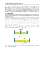
model specifies the topology, i.e. the structure of how the nodes are organized, there
are different topologies to a WSN such as square, star, ad-hoc, irregular Piedrahita et al.
(2010).
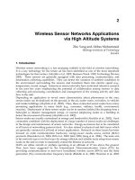
(a) Hardware Layer (b) Application Layer
(c) All Layers
Fig. 1. Hardware, Application Layers and Complete Model Proposal
6.2.2 Middle Layer
The middle layer is responsible to attach a WSN with the needed agents for a specific applica-
tion. Hence this layer has two agents that perform control and resources manage.
• Manager resources Agent (MA): It is a specialized mobile agent that takes decisions
about controlling resources of memory and power. It is aware of required charge for an
agent performs a task, and denies or admits to execute an agent. This is an agent that
takes decisions based on a BDI model Georgeff et al. (1998). Moreover, it says if a group
of tasks can be executed in keeping with the specified hardware.
• Capturing Agent of physical variables (CA): It is a mobile agent that is aware of physical
variables according to a specific application. It takes decisions about propagation and
transmitting of these variables.
6.2.3 Application Layer
The application layer represents specific study case or application for which the WSN is going
to be deployed. Therefore this layer has agents that perform application required tasks.
• Coordinator Agent (CoA): It is an agent aware of required tasks by a study case so it
has a queue of application tasks. Hence, it manages, organizes and negotiates them, for
being executed by a TA successfully. Also, it takes decisions based on a BDI model.
• Tasks Agent (TA): It is a reactive agent that performs tasks assigned by a CoA, as long
as CoA said it had to be.
• Deliberative Agent (DA): It is a mobile agent that takes decisions based on a BDI model
too. It does not need that a CoA manages, organizes and negotiates its tasks, it does
by its own. Accordingly, it performs a set of tasks to achieve its own goal or a goal
established by a MAS which it belongs to.
It is a specific treatment for an application multi-agent system, due to not all sensor nodes

platforms can perform a rational agent i.e. for a simple application there is a group of TA with
a CoA that manages and coordinates entire system, and for a complex application there is a
group of DA that interact to achieve a global goal.
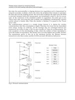
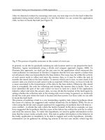
6.3 Interaction Process
First of all, the CoA(or a DA, depending of required type agents) starts the process for assign-
ing a task, it has the belief that a task needs to be done, it has this belief because there is a tasks
list related to the application. Its desire consist of ensure that a task is done successfully by a
TA. Then, its first intention is to interact with MA and to ask task feasibility.
Now, MA beliefs about its hardware characteristics and charge task, and its desire consist to
inform if there are enough resources to do the task, for this reason its intention is reasoning if
charge task processing fits on available resources. It informs true or false.
If MA answer is true, CoA second intention is to create an instance of a TA, and assign this
task. Finally, its last intention is to be sure that the task was done then it asks to TA, if it is
done and depending on this answer it starts with another task or the same.
In the case of DA multi-agent system any DA starts the interaction process with agents in the
middle layer. MA beliefs about its hardware characteristics and charge on a plan (task group).
If MA confirms available resources, the DA starts its process, otherwise it waits until get an
affirmation from MA.
Taking into account above process, we introduce some theoretical formula to determinate
global battery discharge (see Equation 1 and 2) and memory usage (see Equation 3 and 4), for
a time period in the simulation.
B
(t)
= B
(t−1)
− P(C oA)(MA ) − P(TA )L
(t−1)
(1)
B
(t)

= B
(t−1)
− P(DA)(MA) − P (DA )L
(t−1)
(2)
Where B
(t)
is the battery state at time t, P(CoA)(MA) and P(TA) are the processing of CoA
and MA agents and TA agent respectively and L
(t−1)
is the task charge. For equation 2 P(DA)
Smart Wireless Sensor Networks80
and P(MA) are the processing of DA and MA agents and L
(t−1)
is the plan charge. These tasks
and plans are negotiated in a specified order, and constantly repeating.
For Memory usage (M
(t)
), the formula required to perform or not a task or a plan,
M
(t)
= M
(t−1)
− P(C oA)(MA ) − P(TA )L
(t−1)
+ P(TA)L
(t−2)
(3)
M
(t)

= M
(t−1)
− P(DA)(MA) − P (DA )L
(t−1)
+ P(DA)L
(t−2)
(4)
7. Conclusions and future work
The principles, algorithms and application of Distributed Artificial Intelligence can be used
to optimize a network of distributed wireless sensors. The Multi-Agent System approach
permits WSN optimization using rational agents to get this achievement.
It is possible to implement a solution that enables a sensor network to behave as an intelli-
gent multi-agent system through the proposed model due to it utilizes multi-agent systems
together with layered architecture to facilitate intelligence and simulate any WSN, all needed
is to know the final application, where the WSN is going to be deploy. Also, a layered archi-
tecture can provide modularity and structure for a WSN system. Moreover, proposed model
emphasizes about how a WSN works and how to make it intelligent.
From a perspective of multi-agents, artificial societies and simulated organizations, a dis-
tributed sensor network can be installed in an efficient manner and achieve the proposed
objectives of taking measures of physical variables by itself with different types of rational
agents that can be reconfigured to fit any kind of application and measures, also to fit the
most appropriate strategy to achieve requirements of physical variables monitoring.
Further work to do is testing model using a real WSN. Some study cases of multi-agent sys-
tems for specific applications are required to do a complete testing. A useful tool to use is the
Solarium SunSPOT emulator. This emulator makes available a realistic testing to develop and
test SunSPOT devices without requiring hardware platform. After this testing finishes, the
model could be performed over a real WSN of SunSPOT devices.
8. Acknowledgments
This work presents the results of the researches carried out by GIDIA (Artificial Intelligence
Research & Development Group) and GICEI (Scientific & Industrial Instrumentation Research

Group) at the National University of Colombia - Campus Medellin, as advance of two research
projects co-sponsored by DIME (Research Direction of National University of Colombia at
Medellin Campus) and COLCIENCIAS (Colombian Institute of Science and Technology) re-
spectively entitled:"Intelligent Hybrid System Model for Monitoring of Physical variables us-
ing WSN and Multi-Agent Systems" with code 20201007312 and "Development of a model
of intelligent hybrid system for monitoring and remote control of physical variables using
distributed wireless sensor networks" with code 20201007027.
9. References
Cheong, E. (2007). Actor-oriented programming for wireless sensor networks.
Conte, R., Gilbert, N. & Sichman, J. (1998). MAS and social simulation: A suitable commit-
ment, Multi-Agent Systems and Agent-Based Simulation, Springer, pp. 1–9.
CRULLER, D., Estrin, D. & Srivastava, M. (2004). Overview of sensor networks, Computer
37(8): 41–49.
Davoudani, D., Hart, E. & Paechter, B. (2007). An immune-inspired approach to speckled
computing, Artificial Immune Systems pp. 288–299.
Egea-Lopez, E., Vales-Alonso, J., Martinez-Sala, A., Pavon-Marino, P. & Garcia-Haro, J. (2006).
Simulation scalability issues in wireless sensor networks, IEEE Communications Mag-
azine 44(7): 64.
Georgeff, M., Pell, B., Pollack, M., Tambe, M. & Wooldridge, M. (1998). The belief-desire-
intention model of agency, Intelligent Agents V. Agent Theories, Architectures, and
Languages: 5th International Workshop, ATAL’98, Paris, France, July 1998. Proceedings,
Springer, pp. 630–630.
Levis, P., Lee, N., Welsh, M. & Culler, D. (2003). TOSSIM: Accurate and scalable simulation of
entire TinyOS applications, Proceedings of the 1st international conference on Embedded
networked sensor systems, ACM, p. 137.
Moreno, J., Velásquez, J. & Ovalle, D. (2009). Una Aproximación Metodológica para la Con-
strucción de Modelos de Simulación Basados en el Paradigma Multi-Agente, Avances
en Sistemas e Informática 4(2).
O’Hare, G., O’Grady, M. & Marsh, D. (2006). Autonomic wireless sensor networks: Intelligent
ubiquitous sensing, proceeding of ANIPLA 2006, International Congress on Methodolo-

gies for Emerging Technologies in Automation, Publisher, University La Sapienza, Rome,
Italy.
Piedrahita, A., Montoya, A. & Ovalle, D. (2010). Performance Evaluation of an Intelligent
Agents-based Model in WSN with irregular topologies.
Romer, K. & Mattern, F. (2004). The design space of wireless sensor networks, IEEE Wireless
Communications 11(6): 54–61.
Russell, S. & Norving, P. (2003). Artificial Intelligence: A Modern Approach, Prentice-Hall, En-
glewood Cliffs,.
Shah, K., Kumar, M., Inc, S. & Addison, T. (2008). Resource management in wireless sensor
networks using collective intelligence, International Conference on Intelligent Sensors,
Sensor Networks and Information Processing, 2008. ISSNIP 2008, pp. 423–428.
Wang, X., Wang, S. & Jiang, A. (2006). Optimized deployment strategy of mobile agents in
wireless sensor networks, Intelligent Systems Design and Applications, 2006. ISDA’06.
Sixth International Conference on, Vol. 2.
Articial Intelligence for Wireless Sensor Networks Enhancement 81
and P(MA) are the processing of DA and MA agents and L
(t−1)
is the plan charge. These tasks
and plans are negotiated in a specified order, and constantly repeating.
For Memory usage (M
(t)
), the formula required to perform or not a task or a plan,
M
(t)
= M
(t−1)
− P(C oA)(MA ) − P(TA )L
(t−1)
+ P(TA)L
(t−2)

(3)
M
(t)
= M
(t−1)
− P(DA)(MA) − P (DA )L
(t−1)
+ P(DA)L
(t−2)
(4)
7. Conclusions and future work
The principles, algorithms and application of Distributed Artificial Intelligence can be used
to optimize a network of distributed wireless sensors. The Multi-Agent System approach
permits WSN optimization using rational agents to get this achievement.
It is possible to implement a solution that enables a sensor network to behave as an intelli-
gent multi-agent system through the proposed model due to it utilizes multi-agent systems
together with layered architecture to facilitate intelligence and simulate any WSN, all needed
is to know the final application, where the WSN is going to be deploy. Also, a layered archi-
tecture can provide modularity and structure for a WSN system. Moreover, proposed model
emphasizes about how a WSN works and how to make it intelligent.
From a perspective of multi-agents, artificial societies and simulated organizations, a dis-
tributed sensor network can be installed in an efficient manner and achieve the proposed
objectives of taking measures of physical variables by itself with different types of rational
agents that can be reconfigured to fit any kind of application and measures, also to fit the
most appropriate strategy to achieve requirements of physical variables monitoring.
Further work to do is testing model using a real WSN. Some study cases of multi-agent sys-
tems for specific applications are required to do a complete testing. A useful tool to use is the
Solarium SunSPOT emulator. This emulator makes available a realistic testing to develop and
test SunSPOT devices without requiring hardware platform. After this testing finishes, the
model could be performed over a real WSN of SunSPOT devices.

8. Acknowledgments
This work presents the results of the researches carried out by GIDIA (Artificial Intelligence
Research & Development Group) and GICEI (Scientific & Industrial Instrumentation Research
Group) at the National University of Colombia - Campus Medellin, as advance of two research
projects co-sponsored by DIME (Research Direction of National University of Colombia at
Medellin Campus) and COLCIENCIAS (Colombian Institute of Science and Technology) re-
spectively entitled:"Intelligent Hybrid System Model for Monitoring of Physical variables us-
ing WSN and Multi-Agent Systems" with code 20201007312 and "Development of a model
of intelligent hybrid system for monitoring and remote control of physical variables using
distributed wireless sensor networks" with code 20201007027.
9. References
Cheong, E. (2007). Actor-oriented programming for wireless sensor networks.
Conte, R., Gilbert, N. & Sichman, J. (1998). MAS and social simulation: A suitable commit-
ment, Multi-Agent Systems and Agent-Based Simulation, Springer, pp. 1–9.
CRULLER, D., Estrin, D. & Srivastava, M. (2004). Overview of sensor networks, Computer
37(8): 41–49.
Davoudani, D., Hart, E. & Paechter, B. (2007). An immune-inspired approach to speckled
computing, Artificial Immune Systems pp. 288–299.
Egea-Lopez, E., Vales-Alonso, J., Martinez-Sala, A., Pavon-Marino, P. & Garcia-Haro, J. (2006).
Simulation scalability issues in wireless sensor networks, IEEE Communications Mag-
azine 44(7): 64.
Georgeff, M., Pell, B., Pollack, M., Tambe, M. & Wooldridge, M. (1998). The belief-desire-
intention model of agency, Intelligent Agents V. Agent Theories, Architectures, and
Languages: 5th International Workshop, ATAL’98, Paris, France, July 1998. Proceedings,
Springer, pp. 630–630.
Levis, P., Lee, N., Welsh, M. & Culler, D. (2003). TOSSIM: Accurate and scalable simulation of
entire TinyOS applications, Proceedings of the 1st international conference on Embedded
networked sensor systems, ACM, p. 137.
Moreno, J., Velásquez, J. & Ovalle, D. (2009). Una Aproximación Metodológica para la Con-
strucción de Modelos de Simulación Basados en el Paradigma Multi-Agente, Avances

en Sistemas e Informática 4(2).
O’Hare, G., O’Grady, M. & Marsh, D. (2006). Autonomic wireless sensor networks: Intelligent
ubiquitous sensing, proceeding of ANIPLA 2006, International Congress on Methodolo-
gies for Emerging Technologies in Automation, Publisher, University La Sapienza, Rome,
Italy.
Piedrahita, A., Montoya, A. & Ovalle, D. (2010). Performance Evaluation of an Intelligent
Agents-based Model in WSN with irregular topologies.
Romer, K. & Mattern, F. (2004). The design space of wireless sensor networks, IEEE Wireless
Communications 11(6): 54–61.
Russell, S. & Norving, P. (2003). Artificial Intelligence: A Modern Approach, Prentice-Hall, En-
glewood Cliffs,.
Shah, K., Kumar, M., Inc, S. & Addison, T. (2008). Resource management in wireless sensor
networks using collective intelligence, International Conference on Intelligent Sensors,
Sensor Networks and Information Processing, 2008. ISSNIP 2008, pp. 423–428.
Wang, X., Wang, S. & Jiang, A. (2006). Optimized deployment strategy of mobile agents in
wireless sensor networks, Intelligent Systems Design and Applications, 2006. ISDA’06.
Sixth International Conference on, Vol. 2.

Network protocols, architectures and technologies
Part 2
Network protocols,
architectures and technologies

Broadcast protocols for wireless sensor networks 85
Broadcast protocols for wireless sensor networks
Ruiqin Zhao, Xiaohong Shen and Xiaomin Zhang
X

Broadcast protocols for
wireless sensor networks

Ruiqin Zhao, Xiaohong Shen and Xiaomin Zhang
Northwestern Polytechnical University
P.R.China

1. Introduction
Future network is all about an integrated global network based on an open-systems
approach. Integrating different types of wireless networks with wireline backbone networks
seamlessly and the convergence of voice, multimedia, and data traffic over a single IP-based
core network will be the main focus of 4G. With the availability of ultrahigh bandwidth of
up to 100 Mbps, multimedia services can be supported efficiently. Ubiquitous computing is
enabled with enhanced system mobility and portability support, and location-based services
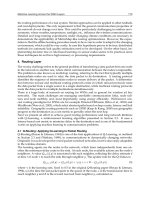
and support of ad hoc networking are expected. Fig. 1 illustrates the networks and
components within the future network architecture. It integrates different network
topologies and platforms. There are two levels of integration: the first is the integration of
heterogeneous wireless networks with varying transmission characteristics such as wireless
LAN (Local Area Network), WAN (Wide Area Network), and PAN (Personal Area
Network) as well as mobile ad hoc networks; the second level includes the integration of
wireless networks and fixed network-backbone infrastructure, the Internet and PSTN
(Public Switched Telephone Network).
Recent advancement in wireless communications and electronics has enabled the
development of low-cost sensor networks. WSN are composed of a large number of sensor
nodes that are densely deployed either inside the phenomenon or very close to it. A wireless
sensor network can be used in a wide variety of commercial and military applications such
as inventory managing, disaster areas monitoring, patient assisting, and target tracking.
The wireless sensor node, being a microelectronic device, can only be equipped with a
limited power source. The issue of energy-efficient communication in WSN has been
attracting attention of many researches during last several years. Broadcasting is a common
operation that allows the node in WSN to share its data efficiently among each other.
Broadcasting can be used for network discovery to initiate the configuration of the network,

to discover multiple routes between a given pair of nodes, and to query for a piece of
desired data in a network (N. B. Chang & M. Liu, 2007). In wireless sensor networks,
broadcasting can serve as an efficient solution for the sensors to share their local
measurements among each other due to the robustness and the effectiveness of the protocol.

5
Smart Wireless Sensor Networks86

Fig. 1. Future network

The traditional way of broadcast in WSN is flooding, which is the straightforward and
obvious way. When a source node has a packet to broadcast in the network, it sends the
packet to all of its neighbors. Then each node that has received the packet for the first time
will rebroadcast the packet to its neighborhood, which leads to the participation of all the
nodes in broadcasting the packet. Thus, the traditional flooding which also is known as
ordinary broadcast mechanism (OBM), results in serious redundancy, collision and
contention, and referred to as broadcast storm problem (S Y Ni et al., 1999). The formation of
the broadcast storm problem is due to the redundancy of rebroadcast which results in the
serious contention and collision. Moreover, the reduction of the redundancy of rebroadcast
is also the requirement of energy-saving in WSN. In networks where each node is assumed
to have a fixed level of transmission power, less rebroadcasts means less energy consumed
with the assumption that the energy needed by receiving is much less than the energy
consumed by transmitting. To save as much energy as possible for each node in the
network, the broadcast algorithm should make as less nodes as possible participate in the
rebroadcast of the broadcasted message (R.Q. Zhao et al.,2007). Therefore, reduction of

rebroadcast redundancy is significant. A satisfying broadcast strategy should be able to
reduce the broadcast redundancy effectively, not only for the saving of bandwidth, but also
for the saving of energy, as both bandwidth and energy are valuable resources in WSN.
While reduction of rebroadcast redundancy is not the only metric for a good broadcast

protocol. There is another metric used for evaluating performance of broadcast protocols
called reachability, which indicates the coverage rate of a broadcast algorithm.
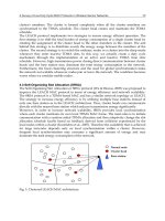
With the aim of solving the broadcast storm problem and maximizing the network life-time,
we propose an efficient broadcast algorithm—Maximum Life-time Localized Broadcast
(ML2B) for WSN, which possesses the following properties:
a) Localized algorithm.
Localized algorithm is distributed algorithm which achieves a desired global objective
with simple local behaviors. Each node makes the decision of rebroadcast based on its
one-hop local information, e.g. its own position, its one-hop neighbors’ information and
energy left in its battery. Distributed design of broadcast routing is required by the
essence of WSN. However, many proposed broadcast approaches were not distributed,
such as those approaches selecting rebroadcast nodes based on a constructed broadcast
tree which could not be maintained by each node using only its own local information.
ML2B need not maintain any global topology information, thus resulting in much less
overhead in WSN.
b) Energy-saving approach.
It is designed with the aim of minimizing energy required per broadcast task and
maximizing network life-time. ML2B is not based on constructing a minimum energy
tree which may cause much overhead to maintain the tree. It selects rebroadcast nodes
by considering the coverage efficiency and the left energy of the node together to
maximize life-time of the whole network. Using the rule of less rebroadcasts results less
total energy consumed, ML2B cuts down the total energy consumption in broadcast
routing by reducing the redundancy of rebroadcast largely which is capable of relieving
the broadcast storm problem synchronously.
c) Degree adaptive broadcast strategy.
To reduce the redundancy of rebroadcast, nodes with large degree will be selected with
higher priority as forward nodes in ML2B. The degree we use in this paper is the
number of left neighbors that have not been covered by the former forward node or by
the broadcast originator. Therefore, the rebroadcast of nodes with high degree brings
high efficiency of the rebroadcast and great reduction of broadcast redundancy.

d) )Fault tolerant algorithm.
For the multi-path and fading effects of the wireless channel, or some sensor nodes may
fail or be blocked due to physical damage or environmental interference, protocols used
in WSN should be robust. This is the reliability or fault tolerance issue. Fault tolerance is
the ability to sustain sensor network functionalities without any interruption due to
sensor node failures. ML2B uses a self-selection mechanism to choose nodes that will
rebroadcast next from nodes that were able to receive the packets without errors.
The remainder of this chapter is organized as follows. Firstly we make a survey of energy
efficient broadcast protocols for wireless sensor networks in Sections 2. Secondly we
propose an efficient broadcast protocol for WSN in Sections 3 and 4. It optimizes
broadcasting by reducing redundant rebroadcasts and balancing the energy consumption
among all nodes. Simulation is done in section 5 to verify the proposed mechanism.
Broadcast protocols for wireless sensor networks 87

Fig. 1. Future network

The traditional way of broadcast in WSN is flooding, which is the straightforward and
obvious way. When a source node has a packet to broadcast in the network, it sends the
packet to all of its neighbors. Then each node that has received the packet for the first time
will rebroadcast the packet to its neighborhood, which leads to the participation of all the
nodes in broadcasting the packet. Thus, the traditional flooding which also is known as
ordinary broadcast mechanism (OBM), results in serious redundancy, collision and
contention, and referred to as broadcast storm problem (S Y Ni et al., 1999). The formation of
the broadcast storm problem is due to the redundancy of rebroadcast which results in the
serious contention and collision. Moreover, the reduction of the redundancy of rebroadcast
is also the requirement of energy-saving in WSN. In networks where each node is assumed
to have a fixed level of transmission power, less rebroadcasts means less energy consumed
with the assumption that the energy needed by receiving is much less than the energy
consumed by transmitting. To save as much energy as possible for each node in the
network, the broadcast algorithm should make as less nodes as possible participate in the

rebroadcast of the broadcasted message (R.Q. Zhao et al.,2007). Therefore, reduction of

rebroadcast redundancy is significant. A satisfying broadcast strategy should be able to
reduce the broadcast redundancy effectively, not only for the saving of bandwidth, but also
for the saving of energy, as both bandwidth and energy are valuable resources in WSN.
While reduction of rebroadcast redundancy is not the only metric for a good broadcast
protocol. There is another metric used for evaluating performance of broadcast protocols
called reachability, which indicates the coverage rate of a broadcast algorithm.
With the aim of solving the broadcast storm problem and maximizing the network life-time,
we propose an efficient broadcast algorithm—Maximum Life-time Localized Broadcast
(ML2B) for WSN, which possesses the following properties:
a) Localized algorithm.
Localized algorithm is distributed algorithm which achieves a desired global objective
with simple local behaviors. Each node makes the decision of rebroadcast based on its
one-hop local information, e.g. its own position, its one-hop neighbors’ information and
energy left in its battery. Distributed design of broadcast routing is required by the
essence of WSN. However, many proposed broadcast approaches were not distributed,
such as those approaches selecting rebroadcast nodes based on a constructed broadcast
tree which could not be maintained by each node using only its own local information.
ML2B need not maintain any global topology information, thus resulting in much less
overhead in WSN.
b) Energy-saving approach.
It is designed with the aim of minimizing energy required per broadcast task and
maximizing network life-time. ML2B is not based on constructing a minimum energy
tree which may cause much overhead to maintain the tree. It selects rebroadcast nodes
by considering the coverage efficiency and the left energy of the node together to
maximize life-time of the whole network. Using the rule of less rebroadcasts results less
total energy consumed, ML2B cuts down the total energy consumption in broadcast
routing by reducing the redundancy of rebroadcast largely which is capable of relieving
the broadcast storm problem synchronously.

c) Degree adaptive broadcast strategy.
To reduce the redundancy of rebroadcast, nodes with large degree will be selected with
higher priority as forward nodes in ML2B. The degree we use in this paper is the
number of left neighbors that have not been covered by the former forward node or by
the broadcast originator. Therefore, the rebroadcast of nodes with high degree brings
high efficiency of the rebroadcast and great reduction of broadcast redundancy.
d) )Fault tolerant algorithm.
For the multi-path and fading effects of the wireless channel, or some sensor nodes may
fail or be blocked due to physical damage or environmental interference, protocols used
in WSN should be robust. This is the reliability or fault tolerance issue. Fault tolerance is
the ability to sustain sensor network functionalities without any interruption due to
sensor node failures. ML2B uses a self-selection mechanism to choose nodes that will
rebroadcast next from nodes that were able to receive the packets without errors.
The remainder of this chapter is organized as follows. Firstly we make a survey of energy
efficient broadcast protocols for wireless sensor networks in Sections 2. Secondly we
propose an efficient broadcast protocol for WSN in Sections 3 and 4. It optimizes
broadcasting by reducing redundant rebroadcasts and balancing the energy consumption
among all nodes. Simulation is done in section 5 to verify the proposed mechanism.
Smart Wireless Sensor Networks88

Simulation results show that the proposed broadcast protocol can prolong the network life-
time of WSN effectively. Finally, in Section 6 we draw the main conclusions.

2. Related Works
The straightforward way of broadcast is flooding. The advantage of flooding is its simplicity
and reliability. However，for its large amount of redundant rebroadcast, flooding will
cause serious packets collision, bandwidth waste，and battery energy exhaustion, which are
referred to as broadcast storm problem (S Y Ni et al., 1999).
Various approaches have been proposed to solve the broadcast storm problem of flooding
for wireless multi-hop networks. Some methods are designed with the aim of alleviating the

broadcast storm problem by reducing redundant broadcasts. As in (J. Wu & F. Dai, 2004) ;
(M. T. Sun &T. H. Lai, 2002); ( W. Peng & X. C. Lu, 2000), each node computes a local cover
set consisting of as less neighbors as possible to cover its whole 2-hop coverage area by
exchanging connectivity information with neighbors. These methods require each node
know its k-hop (k >=2) neighbor information. To maintain the fresh k-hop (k >=2) neighbor
information, these broadcast methods result in heavy overhead on WSN, and they consume
much energy at each node. Some methods (S Y Ni et al., 1999); (M. Lin et al., 1999) select
forward node based on probability, which cannot guarantee the reachability of the
broadcast.
Many proposed energy-saving broadcast methods are centralized, which require the
topology information of the whole network. They try to find a broadcast tree such that the
energy cost of the broadcast tree is minimized. Some methods(J.E. Wieselthier et al., 2000);
(P.J. Wan et al., 2001); (M. Cagalj et al., 2002); ( D. Li et al., 2004) are based on geometry or
graph information of the network to compute the minimum energy tree.
Since the centralized method will cause much overhead in wireless sensor network, some
localized versions of the above algorithms have been proposed recently. The algorithm in
(M. Agarwal et al., 2004) reduces energy consumption by taking advantage of the physical
layer design. (W.Z. Song et al., 2006) proposed a scheme for each node to find the network
topology in a distributed way. However the algorithm proposed in (W.Z. Song et al., 2006),
also requires each node to maintain the network topology, and the overhead is obviously
more than a localized algorithm. The method proposed in (F. Ingelrest & D. Simplot-Ryl.,
2005) requires that each node must be aware of the geometry information within its 2-hop
neighborhood. It results in more control overhead and energy cost than the thorough
distributed algorithm that requires only local one-hop information.
Two types of broadcasting protocols(J P. Sheu g et al., 2006) are proposed for wireless
sensor networks. The two broadcasting protocols, are called one-to-all and all-to-all
broadcasting protocols. And the protocols are proposed for five fixed and regular WSN
topologies. An energy-saving broadcast method using cooperative transmission in WSN is
proposed in (Y W. Hong & A. Scaglione, 2006). The cooperation is provided through a
system called the Opportunistic Large Array (OLA) where network broadcasting is done

through signal processing techniques at the physical layer. In (X. Hui et al., 2006), the
practical models for power aware broadcast in wireless ad hoc and sensor networks are
analyzed. Some literatures deal with the query execution in large sensor networks, e.g. (J P.
Sheu et al., 2007); (C. R. Mann et al., 2007). These proposed protocols are designed to

facilitate any type queries for data content and services over a specific geographic region in
large population, high-density wireless sensor networks. Several robust data delivery
protocols (F. Ye et al., 2005); (Miklós Maróti, 2004) have been proposed for large sensor
networks to disseminate data to interested sensors. GRAdient Broadcast (F. Ye et al., 2005)
addresses the problem of robust data forwarding to a data collecting unit using unreliable
sensor nodes with error-prone wireless channels. A Broadcast Protocol for Sensor networks
(BPS) is proposed in (A. Durres i&V. Paruchuri, 2007). BPS uses the location of each node to
broadcast packets in a distributed way.

3. System Model
The WSN can be abstracted as a graph
( , )G V E
, in whichV is the set of all the nodes in the
network and
E consists of edges presented in the graph. An edge ( , )e u v

, e E exists if
the Euclidean distance between node
u
and
v
is smaller than r , where r is the radius of the
coverage of nodes. We assume all links in the graph is bidirectional, and the graph is in a
connected state. Given a node i , time t is recorded since it receives the broadcasted message
for the first time, and 0t


. The energy left in battery of node i is represented by ( , )e i t . ( , )l i t
is defined as the Euclidean distance between node i and the up-link forward node ( , )uf i t
which sends the broadcasted message.
We assume each node knows its own position information by means of GPS or other
instruments. Each node also obtains its one-hop neighbors’ information which is available in
most location-aided routing ( F. Ingelrest & D. Simplot-Ryl, 2005) of the ad hoc or sensor
networks. Energy left in battery also needs to be provided at every node locally.
For
i V  , several variables are defined as follows:
 Neighbor
( )nb i , is the node that can communicate directly with node i . It is the one-
hop neighbor of node
i .
 Neighbor set
( )
N
B i , is the set of all neighbors of node i .
 Uncovered set
( , )UC i t
, consists of one-hop neighbors that have not been covered by a
certain forward node of the broadcasted message or the broadcast originator, before
t
.
 Degree
( , )d i t , is the number of nodes belonging to ( , )UC i t at
t
. ( , )d i t implies the
rebroadcast efficiency of node
i

. If ( , )d i t is below a threshold before its attempt to
rebroadcast the broadcasted message, node
i
could abandon the attempt.
 Up-link forward node
( , )uf i t , is the ( )nb i that rebroadcasts or broadcasts the message
which is received by node i at
t
(0 ( ))t D i


. Before
( )t D i
, node
i may receive several
copies of the same broadcasted message from different up-link forward nodes(
( )D i is
the add delay of node
i
).
 Down-link forward node
( , )df i t , is the ( )nb i that rebroadcasts the message
at t ( ( ))t D i , after it has received the message from node i . If node i has not
rebroadcasted the message at
( )t D i

, it will not have any down-link forward node.
That is to say, only the forward node has down-link forward node, though except for
broadcast originator node each node owns up-link forward node.
Broadcast protocols for wireless sensor networks 89

Simulation results show that the proposed broadcast protocol can prolong the network life-
time of WSN effectively. Finally, in Section 6 we draw the main conclusions.

2. Related Works
The straightforward way of broadcast is flooding. The advantage of flooding is its simplicity
and reliability. However，for its large amount of redundant rebroadcast, flooding will
cause serious packets collision, bandwidth waste，and battery energy exhaustion, which are
referred to as broadcast storm problem (S Y Ni et al., 1999).
Various approaches have been proposed to solve the broadcast storm problem of flooding
for wireless multi-hop networks. Some methods are designed with the aim of alleviating the
broadcast storm problem by reducing redundant broadcasts. As in (J. Wu & F. Dai, 2004) ;
(M. T. Sun &T. H. Lai, 2002); ( W. Peng & X. C. Lu, 2000), each node computes a local cover
set consisting of as less neighbors as possible to cover its whole 2-hop coverage area by
exchanging connectivity information with neighbors. These methods require each node
know its k-hop (k >=2) neighbor information. To maintain the fresh k-hop (k >=2) neighbor
information, these broadcast methods result in heavy overhead on WSN, and they consume
much energy at each node. Some methods (S Y Ni et al., 1999); (M. Lin et al., 1999) select
forward node based on probability, which cannot guarantee the reachability of the
broadcast.
Many proposed energy-saving broadcast methods are centralized, which require the
topology information of the whole network. They try to find a broadcast tree such that the
energy cost of the broadcast tree is minimized. Some methods(J.E. Wieselthier et al., 2000);
(P.J. Wan et al., 2001); (M. Cagalj et al., 2002); ( D. Li et al., 2004) are based on geometry or
graph information of the network to compute the minimum energy tree.
Since the centralized method will cause much overhead in wireless sensor network, some
localized versions of the above algorithms have been proposed recently. The algorithm in
(M. Agarwal et al., 2004) reduces energy consumption by taking advantage of the physical
layer design. (W.Z. Song et al., 2006) proposed a scheme for each node to find the network
topology in a distributed way. However the algorithm proposed in (W.Z. Song et al., 2006),

also requires each node to maintain the network topology, and the overhead is obviously
more than a localized algorithm. The method proposed in (F. Ingelrest & D. Simplot-Ryl.,
2005) requires that each node must be aware of the geometry information within its 2-hop
neighborhood. It results in more control overhead and energy cost than the thorough
distributed algorithm that requires only local one-hop information.
Two types of broadcasting protocols(J P. Sheu g et al., 2006) are proposed for wireless
sensor networks. The two broadcasting protocols, are called one-to-all and all-to-all
broadcasting protocols. And the protocols are proposed for five fixed and regular WSN
topologies. An energy-saving broadcast method using cooperative transmission in WSN is
proposed in (Y W. Hong & A. Scaglione, 2006). The cooperation is provided through a
system called the Opportunistic Large Array (OLA) where network broadcasting is done
through signal processing techniques at the physical layer. In (X. Hui et al., 2006), the
practical models for power aware broadcast in wireless ad hoc and sensor networks are
analyzed. Some literatures deal with the query execution in large sensor networks, e.g. (J P.
Sheu et al., 2007); (C. R. Mann et al., 2007). These proposed protocols are designed to

facilitate any type queries for data content and services over a specific geographic region in
large population, high-density wireless sensor networks. Several robust data delivery
protocols (F. Ye et al., 2005); (Miklós Maróti, 2004) have been proposed for large sensor
networks to disseminate data to interested sensors. GRAdient Broadcast (F. Ye et al., 2005)
addresses the problem of robust data forwarding to a data collecting unit using unreliable
sensor nodes with error-prone wireless channels. A Broadcast Protocol for Sensor networks
(BPS) is proposed in (A. Durres i&V. Paruchuri, 2007). BPS uses the location of each node to
broadcast packets in a distributed way.

3. System Model
The WSN can be abstracted as a graph
( , )G V E
, in whichV is the set of all the nodes in the
network and

E consists of edges presented in the graph. An edge ( , )e u v , e E exists if
the Euclidean distance between node
u
and
v
is smaller than r , where r is the radius of the
coverage of nodes. We assume all links in the graph is bidirectional, and the graph is in a
connected state. Given a node i , time t is recorded since it receives the broadcasted message
for the first time, and 0t  . The energy left in battery of node
i is represented by ( , )e i t . ( , )l i t
is defined as the Euclidean distance between node i and the up-link forward node ( , )uf i t
which sends the broadcasted message.
We assume each node knows its own position information by means of GPS or other
instruments. Each node also obtains its one-hop neighbors’ information which is available in
most location-aided routing ( F. Ingelrest & D. Simplot-Ryl, 2005) of the ad hoc or sensor
networks. Energy left in battery also needs to be provided at every node locally.
For
i V  , several variables are defined as follows:
 Neighbor
( )nb i , is the node that can communicate directly with node i . It is the one-
hop neighbor of node
i .
 Neighbor set
( )
N
B i , is the set of all neighbors of node i .
 Uncovered set
( , )UC i t
, consists of one-hop neighbors that have not been covered by a
certain forward node of the broadcasted message or the broadcast originator, before

t
.
 Degree
( , )d i t , is the number of nodes belonging to ( , )UC i t at
t
. ( , )d i t implies the
rebroadcast efficiency of node
i
. If ( , )d i t is below a threshold before its attempt to
rebroadcast the broadcasted message, node
i
could abandon the attempt.
 Up-link forward node
( , )uf i t , is the ( )nb i that rebroadcasts or broadcasts the message
which is received by node i at
t
(0 ( ))t D i 
. Before
( )t D i
, node
i may receive several
copies of the same broadcasted message from different up-link forward nodes(
( )D i is
the add delay of node
i
).
 Down-link forward node
( , )df i t , is the ( )nb i that rebroadcasts the message
at t ( ( ))t D i , after it has received the message from node i . If node i has not
rebroadcasted the message at

( )t D i , it will not have any down-link forward node.
That is to say, only the forward node has down-link forward node, though except for
broadcast originator node each node owns up-link forward node.
Smart Wireless Sensor Networks90

 Up-link forward set
( , )UF i t
, is the set of all up-link forward nodes of node i before t . If
it has received the same broadcasted message for
k times before t ( ( ))t D i , its up-link
forward set can be expressed as:



0 1 2 1
( , ) ( , ), ( , ), ( , ) ( , )
k
UF i t uf i t uf i t uf i t uf i t

 , ( 1)k 

(1)

(where
0 1 2
, , t t t ,and
1k
t
 1
( )

k
t t

 records the time node i received the 1st, 2nd, 3rd …,
and
k th copy of the same broadcasted message).
 Down-link forward set
( , )DF i t
, consists of all down-link forward nodes of
node
i
before
t
. Nodes that have not been selected as forward node have an empty
down-link forward set. While the down-link forward set of forward
node
i
with
'
k
down-link forward nodes is given as follows:

'
'
'
0 1 2
1
( , ), ( , ), ( , ) ( , ) , 1
, 0
( , )

k
df i t df i t df i t df i t k
k
DF i t
 
 
 


 







(2)

(where
'
0k  means no rebroadcast is initiated by the rebroadcast of node
i
).

4. Maximum Life-time Localized Broadcast (ML2B) Algorithm
4.1 Design for Add-Delay
( )D i

Utilization of add-delay in broadcast protocols is to reduce the redundancy of nodes’

rebroadcast and energy consumption. When node
i receives a broadcasted message for the
first time, it will not rebroadcast it as OBM. It delays a period of add-delay
( )D i before its
attempt to do the rebroadcast. Even when
( )D i expires, the node will not rebroadcast it
urgently until the node degree
( , ( ))d i D i
is larger than the abandoning threshold n . During
the period time of
0 ( )t D i  ,  node i could abandon its attempt to rebroadcast the
message as soon as its node degree
( , )d i t is equal to or below the threshold, thus reducing
the rebroadcast redundancy and energy consumption largely.
Nodes with larger add-delay have a higher probability of receiving multiple copies of a
certain broadcasted message, before their attempt to rebroadcast. Each reception of the same
message decreases the node degree, thus making nodes with large add-delay rebroadcast
the message with little probability. While nodes with little add-delay may rebroadcast the
message quickly. We assign little add-delay or no-delay to nodes with high rebroadcast
efficiency and enough left energy, large add-delay to nodes with large rebroadcast
redundancy. To formulate the rebroadcast efficiency, two metrics are presented as follows:

( ,0)
( ) , (0 ( ) 1)
d d
a d i
f i f i
a

  

(3)



( ,0)
( ) , (0 ( ) 1)
l l
r l i
f i f i
r


 

(4)

Formula (3) is the node degree metric, and formula (4) is the distance metric.
a
is the
maximum node degree,
r is the radius of nodes’ coverage. It can be induced from the two
formulas that less
( )
l
f
i
or
( )
d

f
i
results in higher rebroadcast efficiency.
To maximize the network life-time, we present the third metric energy metric for selecting
proper rebroadcast nodes. If the left energy at a node is smaller than an energy threshold, it
refuses to forward the broadcasted message. Otherwise, the node calculates the add-delay
based on formula (5) where
E

is the maximum energy when battery is full, and
T
E
is the
energy threshold which is used to prevent nodes with little energy from dying. The selection
of
T
E ’s value affects the performance of ML2B. Too large value will bring low redundancy,
but may result in low reachability simultaneously. Too small value, on the other hand, could
not prevent the premature crash of nodes with less energy left which may affect the
connectivity of WSN. Hence, there is tradeoff in the selection of
T
E ’s value.

( ,0)
( ) , ( ( ,0) )
e T
T
E e i
f
i E e i E

E E




  


(5)

ML2B first introduces a new metrics for the selection of rebroadcast node in WSN. It
incorporates the three metrics presented above together to select rebroadcast nodes with
goals of obtaining low rebroadcast redundancy, high reachability, limited latency, and
maximized network life-time. We propose two different ways to combine node degree,
coverage rate and left energy metrics into a single synthetic metric, based on the product
and sum of the three metrics, respectively. If the product is used, then synthetic metric of
delaying the attempt to rebroadcast the broadcasted message is given by formula (6). The
sum, on the other hand, leads to a new metric shown by formula (7) by suitably selected
values of the three factors:

,

and

.

( ( ,0), ( ,0), ( ,0)) ( ) ( ) ( )
pro
d l e
f

d i l i e i f i f i f i

(6)

( ( ,0), ( ,0), ( ,0)) ( ) ( ) ( )
sum
d l e
f
d i l i e i f i f i f i    

(7)

Nodes with minimized
( ( ,0), ( ,0), ( ,0))f d i l i e i ， rebroadcast the message with the least
latency. We compute the add-delay with the following formula:

( ) . ( ( ,0), ( ,0), ( ,0))D i D f d i l i e i


(8)

(where
D
defines the maximum add-delay, ( ( ,0), ( ,0), ( ,0))f d i l i e i is the synthetic metric
shown by formula (6) or (7) ). Hence, based on formulas: (3)
(8), we can get product and
sum versions of add-delay are:

Broadcast protocols for wireless sensor networks 91

 Up-link forward set
( , )UF i t
, is the set of all up-link forward nodes of node i before t . If
it has received the same broadcasted message for
k times before t ( ( ))t D i , its up-link
forward set can be expressed as:



0 1 2 1
( , ) ( , ), ( , ), ( , ) ( , )
k
UF i t uf i t uf i t uf i t uf i t

 , ( 1)k 

(1)

(where
0 1 2
, , t t t ,and
1k
t

1
( )
k
t t



records the time node i received the 1st, 2nd, 3rd …,
and
k th copy of the same broadcasted message).
 Down-link forward set
( , )DF i t
, consists of all down-link forward nodes of
node
i
before
t
. Nodes that have not been selected as forward node have an empty
down-link forward set. While the down-link forward set of forward
node
i
with
'
k
down-link forward nodes is given as follows:

'
'
'
0 1 2
1
( , ), ( , ), ( , ) ( , ) , 1
, 0
( , )
k
df i t df i t df i t df i t k
k

DF i t
 
 
 




 







(2)

(where
'
0k  means no rebroadcast is initiated by the rebroadcast of node
i
).

4. Maximum Life-time Localized Broadcast (ML2B) Algorithm
4.1 Design for Add-Delay
( )D i

Utilization of add-delay in broadcast protocols is to reduce the redundancy of nodes’
rebroadcast and energy consumption. When node

i receives a broadcasted message for the
first time, it will not rebroadcast it as OBM. It delays a period of add-delay
( )D i before its
attempt to do the rebroadcast. Even when
( )D i expires, the node will not rebroadcast it
urgently until the node degree
( , ( ))d i D i
is larger than the abandoning threshold n . During
the period time of
0 ( )t D i

 ,

node i could abandon its attempt to rebroadcast the
message as soon as its node degree
( , )d i t is equal to or below the threshold, thus reducing
the rebroadcast redundancy and energy consumption largely.
Nodes with larger add-delay have a higher probability of receiving multiple copies of a
certain broadcasted message, before their attempt to rebroadcast. Each reception of the same
message decreases the node degree, thus making nodes with large add-delay rebroadcast
the message with little probability. While nodes with little add-delay may rebroadcast the
message quickly. We assign little add-delay or no-delay to nodes with high rebroadcast
efficiency and enough left energy, large add-delay to nodes with large rebroadcast
redundancy. To formulate the rebroadcast efficiency, two metrics are presented as follows:

( ,0)
( ) , (0 ( ) 1)
d d
a d i
f i f i

a


 

(3)



( ,0)
( ) , (0 ( ) 1)
l l
r l i
f i f i
r

  

(4)

Formula (3) is the node degree metric, and formula (4) is the distance metric.
a
is the
maximum node degree,
r is the radius of nodes’ coverage. It can be induced from the two
formulas that less
( )
l
f
i

or
( )
d
f
i
results in higher rebroadcast efficiency.
To maximize the network life-time, we present the third metric energy metric for selecting
proper rebroadcast nodes. If the left energy at a node is smaller than an energy threshold, it
refuses to forward the broadcasted message. Otherwise, the node calculates the add-delay
based on formula (5) where
E

is the maximum energy when battery is full, and
T
E
is the
energy threshold which is used to prevent nodes with little energy from dying. The selection
of
T
E ’s value affects the performance of ML2B. Too large value will bring low redundancy,
but may result in low reachability simultaneously. Too small value, on the other hand, could
not prevent the premature crash of nodes with less energy left which may affect the
connectivity of WSN. Hence, there is tradeoff in the selection of
T
E ’s value.

( ,0)
( ) , ( ( ,0) )
e T
T

E e i
f
i E e i E
E E




  


(5)

ML2B first introduces a new metrics for the selection of rebroadcast node in WSN. It
incorporates the three metrics presented above together to select rebroadcast nodes with
goals of obtaining low rebroadcast redundancy, high reachability, limited latency, and
maximized network life-time. We propose two different ways to combine node degree,
coverage rate and left energy metrics into a single synthetic metric, based on the product
and sum of the three metrics, respectively. If the product is used, then synthetic metric of
delaying the attempt to rebroadcast the broadcasted message is given by formula (6). The
sum, on the other hand, leads to a new metric shown by formula (7) by suitably selected
values of the three factors:

,

and  .

( ( ,0), ( ,0), ( ,0)) ( ) ( ) ( )
pro
d l e

f
d i l i e i f i f i f i

(6)

( ( ,0), ( ,0), ( ,0)) ( ) ( ) ( )
sum
d l e
f
d i l i e i f i f i f i    
(7)

Nodes with minimized
( ( ,0), ( ,0), ( ,0))f d i l i e i ， rebroadcast the message with the least
latency. We compute the add-delay with the following formula:

( ) . ( ( ,0), ( ,0), ( ,0))D i D f d i l i e i

(8)

(where
D
defines the maximum add-delay, ( ( ,0), ( ,0), ( ,0))f d i l i e i is the synthetic metric
shown by formula (6) or (7) ). Hence, based on formulas: (3)
(8), we can get product and
sum versions of add-delay are:

Smart Wireless Sensor Networks92

[ ( ,0)][ ( ,0)][ ( ,0)]

( )
( )
pro
T
D a d i E e i r l i
D i
E E ar


  



(9)

[ ( ,0)] [ ( ,0)] [ ( ,0)]
( ) ( )
sum
T
a d i r l i E e i
D i D
a r E E


     
  


(10)

4.2 Algorithm Description
ML2B is a delay based broadcast protocol, where add-delay
( )D i is synthetically calculated
based on the only one-hop local information at each node, thus making it a truly distributed
broadcast algorithm. The final important goal of a broadcast routing algorithm is to carry
broadcasted messages to each node in network with as less rebroadcast redundancy as
possible, satisfied reachability and maximized life-time of network. ML2B is designed with
the idea in mind. Let
s
be the broadcast originator, the algorithm flow for  node




i V s 
may be formalized as follows:
 Step 0: Initialization:
1j   , ( )D i D , ( )UF i   .
 Step 1: If node
i has received broadcasted message
s
M
, go to step 2; else if 0j  , go to
step 7, else the node is idle, and stay in step 1.
 Step 2: Check the node ID of originator
s
and the message ID. If
s
M
is a new message,

go to step 3; else, nodei has received the message before, then let 1
j
j  , and go to
step 4.
 Step 3: Let
0t

, and the system time begins. Let 0j

, where
j
indicates the times of
the repeated i ’s reception of
s
M
. Let

( ,0) ( )UC i NB i

(11)

Thus, node degree
( ,0)d i
equals the number of all its neighbors. If
( ,0)e i
is smaller
than an energy threshold
T
E
, node i abandons its attempt to rebroadcast, and go to

step 9.
 Step 4: Let
j
t t , and use
j
t
p to mark the previous-hop node of
s
M
.
j
t
p
transmitted
s
M
at
j
t . We assume the propagation delay can be omitted. Then we get:

( , )
j
j
t
uf i t p
(12)

j
t
p is the

j
th up-link forward node of node i . Add
j
t
p to up-link forward set ( )UF i at last.
 Step 5: Based on the locally obtained position of ( , )
j
uf i t , node i computes the
geographical coverage range of
( , )
j
uf i t which is expressed as ( , )
j
C i t . Then it
updates
( , )
j
UC i t by deleting nodes that locate in ( , )
j
C i t from ( , )
j
UC i t . Based on the
updated
( , )
j
UC i t , nodei could find out its degree ( , )
j
d i t . If ( , )
j
d i t n , it abandons its

attempt to rebroadcast, and go to step 9; else if
0j  go to step 7.

 Step 6:
0j  means node
i
has received
s
M
for the first time. It calculates its add-
delay
( )D i based on three factors: ( ,0)d i , ( ,0)l i and ( ,0)e i . ( ,0)l i equals the Euclidean
distance between node
i and
( ,0)uf i
.
( ,0)d i
has been calculated by step 5, and
( ,0)e i
can
be obtained locally. When we get the value of the three parameters, the add-delay can
be obtained using formula (9) or (10).
 Step 7: Check the current time
t : if
( )t D i

, go to step 1; else let ( , ) ( , )
j
d i t d i t


.
 Step 8: If
( , )
j
d i t n

, node i abandons its attempt to rebroadcast; else rebroadcasts
s
M
to
all its neighbors.
 Step 9: the algorithm ends.
Option for the value of abandoning threshold
n
affects the rebroadcast redundancy and
reachability. There is a tradeoff between the two performance metrics, in which large
n leads
to low reachability, while little one may not achieve as low broadcast redundancy as
large
n could achieve. The value of abandoning threshold can be selected depending upon
the scenarios and applications of WSN.

5. Performance Evaluation
To verify the proposed ML2B, we made lots of simulations using NS-2 (NS-2, 2006) which is
a network simulator supported by DARPA and NSF, with an 802.11 MAC layer. We study
the performance of ML2B in the simulated wireless ad hoc networks. Nodes in the wireless
multi-hop network are placed randomly in a 2-D square area. For all simulation results, each
broadcast stream consists of packets of size 512 bytes and the inter arrival time is uniformly
distributed around a mean rate varying from 2 packets-per-second (pps) to 10 pps
depending upon the simulation scenarios.

In the all simulations made in this paper, we use the formula (10) to calculate the add-delay
for each node by selection that
( ) 2 ( ) 2
d d
f
i f i      . The abandoning threshold and
energy threshold used in our simulations are configured as
/ 5n b

and / 100
T
E E

 , where
b is the average number of neighbors of nodes.

5.1. Performance Metrics Used in Simulations
We consider four performance metrics:
 Saved rebroadcast (SRB):
( ) /
x
y x

, where
x
is the number of nodes that receive the
broadcasted message, and y is the number of nodes that rebroadcasts the message
after their reception of the message.
 Reachability (RE): /
x

z , where z is the number of all nodes in the simulated
connected network. So RE is also known as the coverage rate.
 Maximum end-to-end delay (MED): the interval form the time the broadcasted
message is initiated to the time the last node in the network receiving the message.
 Life-time (LT): the interval from the time the network is initiated to the time the first
node dies.
The saved rebroadcast (SRB) and reachability (RE) metrics were utilized to evaluate the
performance of broadcast algorithms by most of the proposed broadcast approaches (S Y Ni et
al., 1999) ; (D. Katsaros &Y. Manolopoulos, 2006) ; ( F. Ingelrest & D. Simplot-Ryl, 2005) etc.
Broadcast protocols for wireless sensor networks 93

[ ( ,0)][ ( ,0)][ ( ,0)]
( )
( )
pro
T
D a d i E e i r l i
D i
E E ar


  



(9)

[ ( ,0)] [ ( ,0)] [ ( ,0)]
( ) ( )
sum

T
a d i r l i E e i
D i D
a r E E


     
  


(10)

4.2 Algorithm Description
ML2B is a delay based broadcast protocol, where add-delay
( )D i is synthetically calculated
based on the only one-hop local information at each node, thus making it a truly distributed
broadcast algorithm. The final important goal of a broadcast routing algorithm is to carry
broadcasted messages to each node in network with as less rebroadcast redundancy as
possible, satisfied reachability and maximized life-time of network. ML2B is designed with
the idea in mind. Let
s
be the broadcast originator, the algorithm flow for

node




i V s 
may be formalized as follows:

 Step 0: Initialization:
1j

 , ( )D i D

, ( )UF i

 .
 Step 1: If node
i has received broadcasted message
s
M
, go to step 2; else if 0j  , go to
step 7, else the node is idle, and stay in step 1.
 Step 2: Check the node ID of originator
s
and the message ID. If
s
M
is a new message,
go to step 3; else, nodei has received the message before, then let 1
j
j

 , and go to
step 4.
 Step 3: Let
0t

, and the system time begins. Let 0j


, where
j
indicates the times of
the repeated i ’s reception of
s
M
. Let

( ,0) ( )UC i NB i


(11)

Thus, node degree
( ,0)d i
equals the number of all its neighbors. If
( ,0)e i
is smaller
than an energy threshold
T
E
, node i abandons its attempt to rebroadcast, and go to
step 9.
 Step 4: Let
j
t t

, and use
j

t
p to mark the previous-hop node of
s
M
.
j
t
p
transmitted
s
M
at
j
t . We assume the propagation delay can be omitted. Then we get:

( , )
j
j
t
uf i t p


(12)

j
t
p is the
j
th up-link forward node of node i . Add
j

t
p to up-link forward set ( )UF i at last.
 Step 5: Based on the locally obtained position of ( , )
j
uf i t , node i computes the
geographical coverage range of
( , )
j
uf i t which is expressed as ( , )
j
C i t . Then it
updates
( , )
j
UC i t by deleting nodes that locate in ( , )
j
C i t from ( , )
j
UC i t . Based on the
updated
( , )
j
UC i t , nodei could find out its degree ( , )
j
d i t . If ( , )
j
d i t n

, it abandons its
attempt to rebroadcast, and go to step 9; else if

0j  go to step 7.

 Step 6:
0j  means node
i
has received
s
M
for the first time. It calculates its add-
delay
( )D i based on three factors: ( ,0)d i , ( ,0)l i and ( ,0)e i . ( ,0)l i equals the Euclidean
distance between node
i and
( ,0)uf i
.
( ,0)d i
has been calculated by step 5, and
( ,0)e i
can
be obtained locally. When we get the value of the three parameters, the add-delay can
be obtained using formula (9) or (10).
 Step 7: Check the current time
t : if
( )t D i
, go to step 1; else let ( , ) ( , )
j
d i t d i t .
 Step 8: If
( , )
j

d i t n , node i abandons its attempt to rebroadcast; else rebroadcasts
s
M
to
all its neighbors.
 Step 9: the algorithm ends.
Option for the value of abandoning threshold
n
affects the rebroadcast redundancy and
reachability. There is a tradeoff between the two performance metrics, in which large
n leads
to low reachability, while little one may not achieve as low broadcast redundancy as
large
n could achieve. The value of abandoning threshold can be selected depending upon
the scenarios and applications of WSN.

5. Performance Evaluation
To verify the proposed ML2B, we made lots of simulations using NS-2 (NS-2, 2006) which is
a network simulator supported by DARPA and NSF, with an 802.11 MAC layer. We study
the performance of ML2B in the simulated wireless ad hoc networks. Nodes in the wireless
multi-hop network are placed randomly in a 2-D square area. For all simulation results, each
broadcast stream consists of packets of size 512 bytes and the inter arrival time is uniformly
distributed around a mean rate varying from 2 packets-per-second (pps) to 10 pps
depending upon the simulation scenarios.
In the all simulations made in this paper, we use the formula (10) to calculate the add-delay
for each node by selection that
( ) 2 ( ) 2
d d
f
i f i      . The abandoning threshold and

energy threshold used in our simulations are configured as
/ 5n b and / 100
T
E E

 , where
b is the average number of neighbors of nodes.

5.1. Performance Metrics Used in Simulations
We consider four performance metrics:
 Saved rebroadcast (SRB):
( ) /
x
y x , where
x
is the number of nodes that receive the
broadcasted message, and y is the number of nodes that rebroadcasts the message
after their reception of the message.
 Reachability (RE): /
x
z , where z is the number of all nodes in the simulated
connected network. So RE is also known as the coverage rate.
 Maximum end-to-end delay (MED): the interval form the time the broadcasted
message is initiated to the time the last node in the network receiving the message.
 Life-time (LT): the interval from the time the network is initiated to the time the first
node dies.
The saved rebroadcast (SRB) and reachability (RE) metrics were utilized to evaluate the
performance of broadcast algorithms by most of the proposed broadcast approaches (S Y Ni et
al., 1999) ; (D. Katsaros &Y. Manolopoulos, 2006) ; ( F. Ingelrest & D. Simplot-Ryl, 2005) etc.
Smart Wireless Sensor Networks94

5.2. Simulation Results
Performance Dependence on the Network Scale
To study the performance of ML2B under different network scales, we design four scenarios
by placing randomly different number of nodes separately in squares areas of different size,
to maintain a same node density under different network scales. The packets generation rate
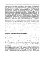
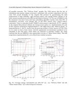
in this experiment is 2 pps. As illustrated in Fig. 2 and Fig. 3, ML2B achieves high saved
rebroadcast without sacrificing the reachability and maximum end-to-end delay under
varying network size. According to expectation, maximum end-to-end delay increases with
the increased network scale. From Fig. 3 we can see that the network with 10 nodes has a
higher SRB than other cases. That is because 10 nodes randomly placed in a 300m×300m
square may be within a node’s coverage area which is larger than the area of the square
(radius of a node’s coverage is 250m). The trend of SRB in the left larger scale networks
becomes flat, due to the same node density.

0
0. 1
0. 2
0. 3
0. 4
10 50 100 200
net wor k nodes
MED ( ms)
ML2B, D=0. 14
ML2B, D=0. 04
OBM

Fig. 2. MED dependence on network scale.

0

0. 2
0. 4
0. 6
0. 8
1
10 50 100 200
net wor k nodes
RE &. SR
B
RE: ML2B, D=0. 14 RE: ML2B, D=0. 04
SRB: ML2B, D=0. 14 SRB: ML2B, D=0. 0
4
OBM

Fig. 3. SRB &. RE dependence on network scale

Performance Dependence on Node Density
We made many experiments to study the ML2B performance dependence on node density.
For the reason of limited pages, we give the results of the network consisting of 50 nodes,
which is shown by Fig. 4 and Fig. 5. The packets generation rate here is 2 pps. Results
illustrated by Fig. 5 shows saved rebroadcast of ML2B fall with the decrease of node density.
That is because the theoretical value of the saved rebroadcast depends upon the node
density. Large density causes big SRB, and ideal SRB will be zero when the node density is
below a certain threshold, which is not the main issue of this paper.

0
0. 1
0. 2
0. 3
0. 4

0. 112 0. 224 0. 448 0. 896
s
q
uar e si ze
(
km^2
)
MED ( ms)
ML2B, D=0. 14
ML2B, D=0. 04
OBM

Fig. 4. MED dependence on node density

0
0. 2
0. 4
0. 6
0. 8
1
0. 112 0. 224 0. 448 0. 896
s
q
uar e si ze
(
km^2
)
RE &. SRB
RE: ML2B, D=0. 14 RE: ML2B, D=0. 04
SRB: ML2B, D=0. 14 SRB: ML2B, D=0. 04

OBM

Fig. 5. SRB &. RE dependence on node density

We also compare the performance of ML2B with maximum add-delay
0.14D  s
and
0.04D  s. From Fig. 2Fig. 5 it is clear that the former outbalanced the latter in SRB and
RE. And both of them have less MED than the OBM in all circumstances. Therefore, in the
following experiments we set 0.14D

s.

Performance Dependence on Packets Generation Rate

0
0. 1
0. 2
0. 3
0. 4
2 4 6 8 10
p
acket
g
ener at i on r at e
( pp
s
)
MED ( ms)
ML2B

OBM

Fig. 6. MED dependence on network load

We study the influence of network load on network performance by varying the packets
generation rate from 2 pps to 10 pps. Simulation results in Fig. 6, Fig. 7 show that increased
network load incurs little impact on ML2B, however leads to increased MED in OBM. ML2B
Broadcast protocols for wireless sensor networks 95

5.2. Simulation Results
Performance Dependence on the Network Scale
To study the performance of ML2B under different network scales, we design four scenarios
by placing randomly different number of nodes separately in squares areas of different size,
to maintain a same node density under different network scales. The packets generation rate
in this experiment is 2 pps. As illustrated in Fig. 2 and Fig. 3, ML2B achieves high saved
rebroadcast without sacrificing the reachability and maximum end-to-end delay under
varying network size. According to expectation, maximum end-to-end delay increases with
the increased network scale. From Fig. 3 we can see that the network with 10 nodes has a
higher SRB than other cases. That is because 10 nodes randomly placed in a 300m×300m
square may be within a node’s coverage area which is larger than the area of the square
(radius of a node’s coverage is 250m). The trend of SRB in the left larger scale networks
becomes flat, due to the same node density.

0
0. 1
0. 2
0. 3
0. 4
10 50 100 200
net wor k nodes

MED ( ms)
ML2B, D=0. 14
ML2B, D=0. 04
OBM

Fig. 2. MED dependence on network scale.

0
0. 2
0. 4
0. 6
0. 8
1
10 50 100 200
net wor k nodes
RE &. SR
B
RE: ML2B, D=0. 14 RE: ML2B, D=0. 04
SRB: ML2B, D=0. 14 SRB: ML2B, D=0. 0
4
OBM

Fig. 3. SRB &. RE dependence on network scale

Performance Dependence on Node Density
We made many experiments to study the ML2B performance dependence on node density.
For the reason of limited pages, we give the results of the network consisting of 50 nodes,
which is shown by Fig. 4 and Fig. 5. The packets generation rate here is 2 pps. Results
illustrated by Fig. 5 shows saved rebroadcast of ML2B fall with the decrease of node density.
That is because the theoretical value of the saved rebroadcast depends upon the node

density. Large density causes big SRB, and ideal SRB will be zero when the node density is
below a certain threshold, which is not the main issue of this paper.

0
0. 1
0. 2
0. 3
0. 4
0. 112 0. 224 0. 448 0. 896
s
q
uar e si ze
(
km^2
)
MED ( ms)
ML2B, D=0. 14
ML2B, D=0. 04
OBM

Fig. 4. MED dependence on node density

0
0. 2
0. 4
0. 6
0. 8
1
0. 112 0. 224 0. 448 0. 896
s

q
uar e si ze
(
km^2
)
RE &. SRB
RE: ML2B, D=0. 14 RE: ML2B, D=0. 04
SRB: ML2B, D=0. 14 SRB: ML2B, D=0. 04
OBM

Fig. 5. SRB &. RE dependence on node density

We also compare the performance of ML2B with maximum add-delay
0.14D  s
and
0.04D  s. From Fig. 2Fig. 5 it is clear that the former outbalanced the latter in SRB and
RE. And both of them have less MED than the OBM in all circumstances. Therefore, in the
following experiments we set 0.14D  s.

Performance Dependence on Packets Generation Rate

0
0. 1
0. 2
0. 3
0. 4
2 4 6 8 10
p
acket
g

ener at i on r at e
( pp
s
)
MED ( ms)
ML2B
OBM

Fig. 6. MED dependence on network load

We study the influence of network load on network performance by varying the packets
generation rate from 2 pps to 10 pps. Simulation results in Fig. 6, Fig. 7 show that increased
network load incurs little impact on ML2B, however leads to increased MED in OBM. ML2B
Smart Wireless Sensor Networks96

maintains nearly as high RE as OBM and, simultaneously achieves SRB with a value larger
than 80%, which reveals the superiority of ML2B over OBM.

0
0. 2
0. 4
0. 6
0. 8
1
2 4 6 8 10
p
acket
g
ener at i on r at e
( pp

s
)
RE &. SRB
RE: ML2B
SRB: ML2B
O
BM

Fig. 7. SRB &. RE dependence on network load

It can be summarized from the above simulations that, ML2B achieves high saved
rebroadcast without sacrificing the reachability and maximum end-to-end delay under all
circumstances. It is beyond our expectation that ML2B, which has delayed the rebroadcast
for an interval of
( )D i , obtains a smaller maximum broadcast end-to-end delay than OBM
that has not delayed rebroadcast. For the different add-delay values for different nodes in
ML2B greatly alleviates and avoids the contention and its resulting collision problem that
persecutes OBM seriously. In ML2B, nodes rebroadcast the message with less contention for
the communication channel, thus making ML2B achieve a smaller maximum end-to-end
delay than OBM. In a word, ML2B could effectively relieve the broadcast storm problem.
Life-Time Evaluation
Fig. 8 shows the network life-time of OBM and ML2B under the same scenario, in which
each node’s initial energy is uniformly distributed between 0.5 J (joule) and 1.0 J. The first
and last node dies separately at 32.48 s and 33.62 s in OBM. After 33.62 s no node dies due to
malfunction of the broadcast caused by the unconnectivity of WSN due to the too much
dead nodes. While in ML2B, they happen at 73.05 s and 95.0 s separately. Life-time is
defined as the interval from the time WSN was initiated to the time the first node died.
Obviously, ML2B has more than doubles the useful network life-time compared with OBM.

0

20
40
60
80
100
0 30 32.9 33.4 60 74.6 79.4 80.9 94 97 100
time (s)
nodes still aliv
e
ML2B
OBM

Fig. 8. Number of nodes still alive in the network of 100 nodes

We break the whole simulation time into many small time steps which also are called as
rounds. Broadcast originator broadcasts each packet to other nodes in the network during
each round. Table.1 shows the network life-time by round with different initial energy,
which manifests ML2B obtains much longer network life-time than OBM under different
initial energy.

Energy
(J/node)

Protocol Life-Time
(rounds)
0.25 ML2B 192
OBM
45
0.5
ML2B 245

OBM 91
1.0
ML2B 407
OBM
195
Table 1. life-time using different amount of initial energy

6. Conclusion
This paper focused on the broadcasting design of wireless multi-hop networks. When a
node has packets to broadcast in the network, the broadcast protocol should route these
packets to all nodes in the network with little overhead, latency, and consumed energy. To
alleviate the broadcast storm problem and simultaneously maximize the network life-time,
we propose a new and efficient broadcast protocol Maximum Life-time Localized
Broadcast (ML2B) for WSN such as wireless ad hoc and sensor networks. ML2B is featured
by the following properties: effective reduction of the rebroadcast redundancy, adaptation
to node degree, energy conservation, and synthetic consideration of node degree, coverage
rate and left energy when selecting rebroadcast nodes. ML2B is based on add-delay strategy
which is adopted from the delay-based geographical routing (M. Mauve et al., 2001); (B.
Blum et al., 2003) in wireless ad hoc networks. However, the add-delay strategy used in
ML2B is different from that used in the geographical routing. The main goal of add-delay
here is to select applicable rebroadcast nodes to achieve high broadcast efficiency without
sacrificing the network life-time. We also proposed two methods to calculate the add-delay.
To further reduce the rebroadcast redundancy and maximize the network life-time, ML2B
has defined two thresholds: abandoning threshold and energy threshold. The former makes
nodes with little uncovered neighbors abandon their rebroadcast, and the latter makes
nodes with very little energy left in their batteries refuse to rebroadcast messages. The two
thresholds could save a number of unused rebroadcasts, decrease the needed total energy
for a message broadcast, and extend the network life-time consequently.
Simulations results have verified the effectiveness of ML2B through different ways, which
manifest that ML2B achieves high saved rebroadcast with lower maximum end-to-end delay

than OBM without sacrificing the reachability under all circumstances. And simultaneously,
it has more than doubles the useful network life-time compared with OBM.
However, there are still some works left in ML2B. E.g., the formulas for the add-delay
calculation may also needs some improvements. We only simulate the sum version the
synthetic metric for the selection of broadcast nodes. The product version synthetic metric
Broadcast protocols for wireless sensor networks 97

maintains nearly as high RE as OBM and, simultaneously achieves SRB with a value larger
than 80%, which reveals the superiority of ML2B over OBM.

0
0. 2
0. 4
0. 6
0. 8
1
2 4 6 8 10
p
acket
g
ener at i on r at e
( pp
s
)
RE &. SR
B
RE: ML2B
SRB: ML2B
O
BM

Fig. 7. SRB &. RE dependence on network load

It can be summarized from the above simulations that, ML2B achieves high saved
rebroadcast without sacrificing the reachability and maximum end-to-end delay under all
circumstances. It is beyond our expectation that ML2B, which has delayed the rebroadcast
for an interval of
( )D i , obtains a smaller maximum broadcast end-to-end delay than OBM
that has not delayed rebroadcast. For the different add-delay values for different nodes in
ML2B greatly alleviates and avoids the contention and its resulting collision problem that
persecutes OBM seriously. In ML2B, nodes rebroadcast the message with less contention for
the communication channel, thus making ML2B achieve a smaller maximum end-to-end
delay than OBM. In a word, ML2B could effectively relieve the broadcast storm problem.
Life-Time Evaluation
Fig. 8 shows the network life-time of OBM and ML2B under the same scenario, in which
each node’s initial energy is uniformly distributed between 0.5 J (joule) and 1.0 J. The first
and last node dies separately at 32.48 s and 33.62 s in OBM. After 33.62 s no node dies due to
malfunction of the broadcast caused by the unconnectivity of WSN due to the too much
dead nodes. While in ML2B, they happen at 73.05 s and 95.0 s separately. Life-time is
defined as the interval from the time WSN was initiated to the time the first node died.
Obviously, ML2B has more than doubles the useful network life-time compared with OBM.

0
20
40
60
80
100
0 30 32.9 33.4 60 74.6 79.4 80.9 94 97 100
time (s)

nodes still aliv
e
ML2B
OBM

Fig. 8. Number of nodes still alive in the network of 100 nodes

We break the whole simulation time into many small time steps which also are called as
rounds. Broadcast originator broadcasts each packet to other nodes in the network during
each round. Table.1 shows the network life-time by round with different initial energy,
which manifests ML2B obtains much longer network life-time than OBM under different
initial energy.

Energy
(J/node)

Protocol Life-Time
(rounds)
0.25 ML2B 192
OBM 45
0.5 ML2B 245
OBM 91
1.0 ML2B 407
OBM 195
Table 1. life-time using different amount of initial energy

6. Conclusion
This paper focused on the broadcasting design of wireless multi-hop networks. When a
node has packets to broadcast in the network, the broadcast protocol should route these
packets to all nodes in the network with little overhead, latency, and consumed energy. To

alleviate the broadcast storm problem and simultaneously maximize the network life-time,
we propose a new and efficient broadcast protocol Maximum Life-time Localized
Broadcast (ML2B) for WSN such as wireless ad hoc and sensor networks. ML2B is featured
by the following properties: effective reduction of the rebroadcast redundancy, adaptation
to node degree, energy conservation, and synthetic consideration of node degree, coverage
rate and left energy when selecting rebroadcast nodes. ML2B is based on add-delay strategy
which is adopted from the delay-based geographical routing (M. Mauve et al., 2001); (B.
Blum et al., 2003) in wireless ad hoc networks. However, the add-delay strategy used in
ML2B is different from that used in the geographical routing. The main goal of add-delay
here is to select applicable rebroadcast nodes to achieve high broadcast efficiency without
sacrificing the network life-time. We also proposed two methods to calculate the add-delay.
To further reduce the rebroadcast redundancy and maximize the network life-time, ML2B
has defined two thresholds: abandoning threshold and energy threshold. The former makes
nodes with little uncovered neighbors abandon their rebroadcast, and the latter makes
nodes with very little energy left in their batteries refuse to rebroadcast messages. The two
thresholds could save a number of unused rebroadcasts, decrease the needed total energy
for a message broadcast, and extend the network life-time consequently.
Simulations results have verified the effectiveness of ML2B through different ways, which
manifest that ML2B achieves high saved rebroadcast with lower maximum end-to-end delay
than OBM without sacrificing the reachability under all circumstances. And simultaneously,
it has more than doubles the useful network life-time compared with OBM.
However, there are still some works left in ML2B. E.g., the formulas for the add-delay
calculation may also needs some improvements. We only simulate the sum version the
synthetic metric for the selection of broadcast nodes. The product version synthetic metric
Smart Wireless Sensor Networks98

shown by formula (9) will be investigated and simulated in the future work to evaluate its
performances.

7. Acknowledgements

The first author would like to acknowledge helpful discussion and solid support from the
co-authors of the chapter.
This work was supported by NPU Foundation for Fundamental Research (NPU-FFR-
JC201004).

8. References
A. Durresi, V. Paruchuri, “Broadcast protocol for energy-constrained networks,” IEEE
Transactions on Broadcasting, vol. 53, no. 1, Mar. 2007, pp. 112-119.
B. Blum, T. He, S. Son, J. Stankovic. IGF: A State-free Robust Communication Protocol for
Wireless Sensor Networks. Department of Computer Science, University of
Virginia, USA, Tech. Rep. CS-2003-11, 2003.
C. R. Mann, R. O. Baldwin, J. P. Kharoufeh, and B. E. Mullins, “A trajectory-based selective
broadcast query protocol for large-scale, high-density wireless sensor networks,”
Telecommunication System, vol. 35, no. 1-2, Jun. 2007, pp. 67–86.
D. Li, X. Jia, and H. Liu, “Minimum energy-cost broadcast routing in static ad hoc wireless
networks,” IEEE Transactions on Mobile Computing, vol. 3, no. 2, Apr Jun. 2004.
F. Ingelrest and D. Simplot-Ryl, “Localized broadcast incremental power protocol for
wireless ad hoc networks,” Proc. IEEE ISCC, 2005.
F. Ye, G. Zhong, S. Lu, and L. Zhang, “GRAdient broadcast: a robust data delivery protocol for
large scale sensor networks,” Wireless Networks, vol. 11, no. 3, May 2005, pp. 285–298.
J.E. Wieselthier, G.D. Nguyen, and A. Ephremides, “On the construction of energy-efficient
broadcast and multicast trees in wireless networks,” Proc. IEEE INFOCOM, 2000.
J P. Sheu, C S. Hsu and Y J. Chang, “Efficient broadcasting protocols for regular wireless
sensor networks,” Wireless Communications and Mobile Computing, vol. 6, no. 1,
2006, pp. 35–48.
J P. Sheu, S C. Tu, and C H. Yu, “A distributed query protocol in wireless sensor networks,”
Wireless Personal Communications, vol. 41, no.4, Jun. 2007, pp. 449–464.
J. Wu and F. Dai, “A generic distributed broadcast scheme in ad hoc wireless networks,”
IEEE Transactions on Computers, vol. 53, no. 10, Oct. 2004, pp. 1343-1354.
M. Agarwal, J. H. Cho, L. Gao, and J. Wu, “Energy efficient broadcast in wireless ad hoc

networks with hitch-hiking,” Proc. IEEE INFOCOM, 2004.
M. Cagalj, J.P. Hubaux, and C. Enz, “Minimum-energy broadcast in all-wireless networks:
NP-completeness and distribution issues,” Proc. MOBICOM, 2002.
Miklós Maróti, “Directed flood-routing framework for wireless sensor networks,” Proc. IFIP
International Federation for Information, LNCS 3231, 2004, pp. 99–114.
M. Lin, K. Marzullo and S. Masini, “Gossip versus deterministic flooding: Low packet overhead
and high reliability for broadcasting on small networks.” UCSD Tech. Rep. 0637, 1999.
M. Mauve, J. Widmer, H. Hartenstein. A Survey on Position-Based Routing in Mobile Ad
Hoc Networks. IEEE Network. pp. 30-39, Nov. /Dec. 2001.

M T. Sun and T H. Lai, “Location aided broadcast in wireless ad hoc network systems,”
Proc. IEEE WCNC, 2002, pp. 597- 602.
N. B. Chang, and M. Liu, “Controlled flooding search in a large network,” IEEE/ACM
Transactions on Networking, vol. 15, no. 2, Apr. 2007, pp. 436-449.
NS-2 Network Simulator , Jun. 2009
P.J. Wan, G. Calinescu, X.Y. Li, and O. Frieder, “Minimum-energy broadcast routing in static
ad hoc wireless networks,” Proc. IEEE INFOCOM, 2001.
R.Q. Zhao et al., Maximum Life-time Localized Broadcast Routing in MANET. Lecture
Notes in Computer Science, 2007, 4672(1): 193–202.
S Y Ni, Y C Tseng, Y S Chen, J P Sheu. The Broadcast Storm problem in a Mobile Ad Hoc
Network. Proceedings of the Fifth Annual ACM/ IEEE International Conference on
Mobile Computing and network .Washington: IEEE, pp. 151–162, 1999
W. Peng and X C. Lu, “On the reduction of broadcast redundancy in mobile ad hoc
networks,” Proc. MOBIHOC, 2000, pp. 129-130.
W.Z. Song, X. Y. Li, and W. Z. Wang, “Localized topology control for unicast and broadcast
in wireless ad hoc networks,” IEEE Transactions on Parallel and Distributed
Systems, vol. 17, no. 4, 2006, pp. 321-334.
X. Hui, M. Jeon, S. Lei, N. Yu, J. Cho, and S. Lee, “Impact of practical models on power
aware broadcast protocols for wireless ad hoc and sensor networks,” Proc. IEEE
Workshop on SEUS–CCIA, 2006.

Y W. Hong and A. Scaglione, “Energy-Efficient Broadcasting with Cooperative
Transmissions in Wireless Sensor Networks,” IEEE Transactions on Wireless
Communications, vol. 5, no. 10, Oct. 2006, pp. 2844-2855.
Broadcast protocols for wireless sensor networks 99

shown by formula (9) will be investigated and simulated in the future work to evaluate its
performances.

7. Acknowledgements
The first author would like to acknowledge helpful discussion and solid support from the
co-authors of the chapter.
This work was supported by NPU Foundation for Fundamental Research (NPU-FFR-
JC201004).

8. References
A. Durresi, V. Paruchuri, “Broadcast protocol for energy-constrained networks,” IEEE
Transactions on Broadcasting, vol. 53, no. 1, Mar. 2007, pp. 112-119.
B. Blum, T. He, S. Son, J. Stankovic. IGF: A State-free Robust Communication Protocol for
Wireless Sensor Networks. Department of Computer Science, University of
Virginia, USA, Tech. Rep. CS-2003-11, 2003.
C. R. Mann, R. O. Baldwin, J. P. Kharoufeh, and B. E. Mullins, “A trajectory-based selective
broadcast query protocol for large-scale, high-density wireless sensor networks,”
Telecommunication System, vol. 35, no. 1-2, Jun. 2007, pp. 67–86.
D. Li, X. Jia, and H. Liu, “Minimum energy-cost broadcast routing in static ad hoc wireless
networks,” IEEE Transactions on Mobile Computing, vol. 3, no. 2, Apr Jun. 2004.
F. Ingelrest and D. Simplot-Ryl, “Localized broadcast incremental power protocol for
wireless ad hoc networks,” Proc. IEEE ISCC, 2005.
F. Ye, G. Zhong, S. Lu, and L. Zhang, “GRAdient broadcast: a robust data delivery protocol for
large scale sensor networks,” Wireless Networks, vol. 11, no. 3, May 2005, pp. 285–298.
J.E. Wieselthier, G.D. Nguyen, and A. Ephremides, “On the construction of energy-efficient

broadcast and multicast trees in wireless networks,” Proc. IEEE INFOCOM, 2000.
J P. Sheu, C S. Hsu and Y J. Chang, “Efficient broadcasting protocols for regular wireless
sensor networks,” Wireless Communications and Mobile Computing, vol. 6, no. 1,
2006, pp. 35–48.
J P. Sheu, S C. Tu, and C H. Yu, “A distributed query protocol in wireless sensor networks,”
Wireless Personal Communications, vol. 41, no.4, Jun. 2007, pp. 449–464.
J. Wu and F. Dai, “A generic distributed broadcast scheme in ad hoc wireless networks,”
IEEE Transactions on Computers, vol. 53, no. 10, Oct. 2004, pp. 1343-1354.
M. Agarwal, J. H. Cho, L. Gao, and J. Wu, “Energy efficient broadcast in wireless ad hoc
networks with hitch-hiking,” Proc. IEEE INFOCOM, 2004.
M. Cagalj, J.P. Hubaux, and C. Enz, “Minimum-energy broadcast in all-wireless networks:
NP-completeness and distribution issues,” Proc. MOBICOM, 2002.
Miklós Maróti, “Directed flood-routing framework for wireless sensor networks,” Proc. IFIP
International Federation for Information, LNCS 3231, 2004, pp. 99–114.
M. Lin, K. Marzullo and S. Masini, “Gossip versus deterministic flooding: Low packet overhead
and high reliability for broadcasting on small networks.” UCSD Tech. Rep. 0637, 1999.
M. Mauve, J. Widmer, H. Hartenstein. A Survey on Position-Based Routing in Mobile Ad
Hoc Networks. IEEE Network. pp. 30-39, Nov. /Dec. 2001.

M T. Sun and T H. Lai, “Location aided broadcast in wireless ad hoc network systems,”
Proc. IEEE WCNC, 2002, pp. 597- 602.
N. B. Chang, and M. Liu, “Controlled flooding search in a large network,” IEEE/ACM
Transactions on Networking, vol. 15, no. 2, Apr. 2007, pp. 436-449.
NS-2 Network Simulator , Jun. 2009
P.J. Wan, G. Calinescu, X.Y. Li, and O. Frieder, “Minimum-energy broadcast routing in static
ad hoc wireless networks,” Proc. IEEE INFOCOM, 2001.
R.Q. Zhao et al., Maximum Life-time Localized Broadcast Routing in MANET. Lecture
Notes in Computer Science, 2007, 4672(1): 193–202.
S Y Ni, Y C Tseng, Y S Chen, J P Sheu. The Broadcast Storm problem in a Mobile Ad Hoc
Network. Proceedings of the Fifth Annual ACM/ IEEE International Conference on

Mobile Computing and network .Washington: IEEE, pp. 151–162, 1999
W. Peng and X C. Lu, “On the reduction of broadcast redundancy in mobile ad hoc
networks,” Proc. MOBIHOC, 2000, pp. 129-130.
W.Z. Song, X. Y. Li, and W. Z. Wang, “Localized topology control for unicast and broadcast
in wireless ad hoc networks,” IEEE Transactions on Parallel and Distributed
Systems, vol. 17, no. 4, 2006, pp. 321-334.
X. Hui, M. Jeon, S. Lei, N. Yu, J. Cho, and S. Lee, “Impact of practical models on power
aware broadcast protocols for wireless ad hoc and sensor networks,” Proc. IEEE
Workshop on SEUS–CCIA, 2006.
Y W. Hong and A. Scaglione, “Energy-Efficient Broadcasting with Cooperative
Transmissions in Wireless Sensor Networks,” IEEE Transactions on Wireless
Communications, vol. 5, no. 10, Oct. 2006, pp. 2844-2855.

Routing Protocol with Unavailable Nodes in Wireless Sensor Networks 101
Routing Protocol with Unavailable Nodes in Wireless Sensor Networks
Deyun Gao, Linjuan Zhang and Yingying Gong
0
Routing Protocol with Unavailable
Nodes in Wireless Sensor Networks
Deyun Gao, Linjuan Zhang and Yingying Gong
National Engineering Laboratory for Next Generation Internet Interconnection Devices,
School of Electronic and Information Engineering, Beijing Jiaotong University
Beijing 100044, P.R.China
1. Introduction
With the rapid development of modern microelectronic technology, wireless communication
technology, signal processing technology, and computer network technology, wireless sensor
networks (WSNs) has become one of the most important and the most basic technologies of
information access (Jennifer Yick, 2008). WSNs have been widely used in military, environ-
ment monitoring, medicine care and transportation control. Routing protocol is one of the key
support technologies in WSNs and the performance of routing protocols significantly impact

the performance of the entire network (Khan & Javed, 2008).
In wireless sensor networks (WSNs), some unavailable areas often are formed because some
sensor nodes become unavailable due to energy exhausted, congestion, or disaster (Fang et al.,
2006; Jafarian & Jaseemuddin, 2008). Multi-path routing protocol is one of the mechanisms to
solve or alleviate the above problems. Data delivery over multiple paths can help balance net-
work load and extend the life time of entire network. Generally, multiple paths in the routing
protocols can be classified into two categories: disjoint multiple paths and joint multiple paths
(Ganesan et al., 2001). Disjoint multiple paths can be furthermore classified into node-disjoint
multiple paths and link-disjoint multiple paths. In the node-disjoint multiple paths, each path
is independent and has no affect on each other. Apparently, it is better to choose node-disjoint
multiple paths for data delivery in the designed routing protocol if possible.
Most of multi-path routing protocols in wireless ad hoc networks are extended from classi-
cal single path routing protocols. For example, split multi-path routing (SMR) is based on
the dynamic source routing (DSR) protocol and ad hoc on demand multi-path distance vector
routing (AOMDV) extends the ad hoc on-demand distance vector routing (AODV) protocol
(Lee & Gerla, 2001; Marina & Das, 2001). Similarly, as its special type, most of multi-path
routing protocols in WSNs are extended from the ones in wireless ad hoc networks and at
the same time take account of different factors such as energy, QoS, security, congestion, and
etc. There are many papers to consider energy efficiency when designing multi-path routing
protocols in WSNs (KIM et al., 2008). They mainly select multiple paths based on the link cost
function consisting of both the node residual energy level and hop count. In (Huang & Fang,
2008), Xiaoxia Huang and Yuguang Fang proposed a probabilistic modeling of link state for
wireless sensor networks. Based on this model, an approximation of local multi-path rout-
ing algorithm is explored to provide soft-QoS under multiple constraints, such as delay and
reliability. Yunfeng Chen and Nidal Nasser proposed to select multiple paths between one
6
Smart Wireless Sensor Networks102
sink and multiple sources with the consideration of reducing collision occurred at nodes that
are receiving and forwarding packets on behalf of the source nodes in order to improve QoS
(Chen & Nasser, 2008). The same authors proposed an secure and energy-efficient multi-path

routing protocol (SEER) (Nasser & Chen, 2007). Besides of using multiple paths alternately for
communication between two nodes to prolong the lifetime of the network, SEER is resistive
some specific attacks that have the character of pulling all traffic through the malicious nodes
by advertising an attractive route to the destination. In (Toledo & Wang, 2006), Alberto Lopez
Toledo and Xiaodong Wang proposed to use network coding to achieve an adaptive equiva-
lent solution to the construction of disjoint multi-path routes from a source to a destination.
It exploits both the low cost mesh-topology construction, such as those obtained by diffusion
algorithms, and the capacity achieving capability of linear network coding. Jenn-Yue Teo,
Yajun Ha, and Chen-Khong Tham proposed a heuristics-based interference-minimized multi-
path routing (I2MR) protocol that increases throughput by discovering and using maximally
zone-disjoint shortest paths for load balancing and a congestion control scheme that is able to
adjust the loading rate of the source dynamically (Teo et al., 2008).
However, the existed multi-path routing protocols can not provide mechanisms to cross
around the unavailable areas particularly during the routing building procedure or later data
delivering procedure. Because in WSNs the states of sensor nodes or areas are changing due to
many factors, it is important to consider all of these factors and situations when designing the
routing protocols. In this chapter, we propose a new micro sensor multi-path routing protocol
(MSMRP) to avoid crossing the unavailable areas based on the micro sensor routing protocol
(MSRP) previously developed by us (Gao et al., 2009). We firstly define the unavailable areas
that may be formed due to kinds of reasons such as energy exhausted, disaster and so on,
which can be detected by kinds of sensors through some predefined settings. Then we design
several new routing packets and routing tables to help building multiple paths based on the
MSRP. In particularly, we propose a neighbor node table exchanging mechanism that can help
build an alternate route around the unavailable areas and try to avoid the multiple paths in-
tersect. When a sensor node becomes unavailable during the route reply (RREP) forwarding
procedure, its precursor node will try to find the alternate route to forward the RREP to the
destination with the help of above mechanism. It also can help balance the network load, im-
prove the transmission efficiency and routing stability with multi-path transmission, which
furthermore decreases the unavailable areas’ forming and enlarging. Finally, we implement
the proposed protocol in the real sensor nodes and set up a testbed to conduct detail exper-

iments. The experimental results show that MSMRP can perform well to build up multiple
paths to avoid the unavailable areas.
This chapter is organized as follows. Section 2 describes the MSRP routing protocol. Section 3
introduces the definitions of unavailable and available areas, and presents the details of the
MSMRP including new added message formats and operation mechanisms. Section 4 intro-
duces our developed sensor node’s hardware architecture. Section 5 presents the software
architecture, operation mechanisms of some standard interfaces of the connector module and
adaptive data processing scheme. Section 6 shows the experimental performance results of
WSNs implementing MSMRP. Some important conclusions are drawn in Section 7.
2. Micro Sensor Routing Protocol
Based on AODV, we designed Micro Sensor Routing Protocol (MSRP)for IEEE802.15.4 based
sensor network. In the following, we firstly describe the protocol stacks of IPv6 sensor node
designed. Then, we present the details of MSRP.
2.1 Protocol Stack of IPv6 sensor node
Fig. 1 shows protocol stack of IPv6 sensor node designed by us. We divide the protocols into
fiver layers including application layer, network layer, adaptation layer, data link layer and
physical layer. Considering scare resources we simplify the traditional transportation layer
(TCP and UDP) and merge them into network layer. Also, we put our MSRP routing protocol
into network layer. Specially, we add a new adaption layer. For other layers, it is easy to
understand their functions and we do not need to introduce them. Here, we just describe the
adaptation layer.
IEEE 802.15.4 PHY
IEEE 802.15.4 MAC Layer
Adaptation Layer
IPv6 MSRP
Routing Protocol
IPv6 Protocol
UDP
TCP
ICMPv6

ND
IPv6 Micro
Protocol Stack
Service
Discovery
IPv6 Application
Application
Layer
Network Layer
Data Link
Layer
Physical Layer
Adapatation
Layer
Fig. 1. Architecture of IPv6 Wireless Sensor Node
The adaptation layer lies between IEEE 802.15.4 MAC layer and the network layer. Adapta-
tion layer is used mainly for fragmentation and reassembly. As we use IPv6 in the network
layer, the maximum transmission unit (MTU) size for IPv6 packets over IEEE802.15.4 is 1280
octets. However, a full IPv6 packet does not fit in an IEEE802.15.4 frame. IEEE802.15.4 pro-
tocol data units have different sizes depending on how much overhead is present. Starting
from a maximum physical layer packet size of 127 octets and a maximum frame overhead of
25, the resultant maximum frame size at the media access control layer is 102 octets. Link-
layer security imposes further overhead, which in the maximum case (21 octets of overhead
in the AES-CCM-128 case, versus 9 and 13 for AES-CCM-32 and AES-CCM-64, respectively)
leaves only 81 octets available. This is obviously far below the maximum IPv6 packet size
of 1280 octets, and in keeping with Section 5 of the IPv6 specification (Deering & Hinden,
1998), a fragmentation and reassembly adaptation layer must be provided at the layer below
IP. Furthermore, since the IPv6 header is 40 octets long, this leaves only 41 octets for upper-
layer protocols, like UDP. The latter uses 8 octets in the header which leaves only 33 octets for
application data. Thus, there is a need for a fragmentation and reassembly layer.

2.2 Micro Sensor Routing Protocol Packet Format
In order to reduce low-speed IPv6 WSN equipment energy consumption, it is very important
to design efficient and streamlined routing protocol packet formats. Considering low-speed
wireless network characteristics, we designed our routing protocol with three routing packet
formats including routing request (RREQ), routing reply (RREP) and routing error (RERR). We
Routing Protocol with Unavailable Nodes in Wireless Sensor Networks 103
sink and multiple sources with the consideration of reducing collision occurred at nodes that
are receiving and forwarding packets on behalf of the source nodes in order to improve QoS
(Chen & Nasser, 2008). The same authors proposed an secure and energy-efficient multi-path
routing protocol (SEER) (Nasser & Chen, 2007). Besides of using multiple paths alternately for
communication between two nodes to prolong the lifetime of the network, SEER is resistive
some specific attacks that have the character of pulling all traffic through the malicious nodes
by advertising an attractive route to the destination. In (Toledo & Wang, 2006), Alberto Lopez
Toledo and Xiaodong Wang proposed to use network coding to achieve an adaptive equiva-
lent solution to the construction of disjoint multi-path routes from a source to a destination.
It exploits both the low cost mesh-topology construction, such as those obtained by diffusion
algorithms, and the capacity achieving capability of linear network coding. Jenn-Yue Teo,
Yajun Ha, and Chen-Khong Tham proposed a heuristics-based interference-minimized multi-
path routing (I2MR) protocol that increases throughput by discovering and using maximally
zone-disjoint shortest paths for load balancing and a congestion control scheme that is able to
adjust the loading rate of the source dynamically (Teo et al., 2008).
However, the existed multi-path routing protocols can not provide mechanisms to cross
around the unavailable areas particularly during the routing building procedure or later data
delivering procedure. Because in WSNs the states of sensor nodes or areas are changing due to
many factors, it is important to consider all of these factors and situations when designing the
routing protocols. In this chapter, we propose a new micro sensor multi-path routing protocol
(MSMRP) to avoid crossing the unavailable areas based on the micro sensor routing protocol
(MSRP) previously developed by us (Gao et al., 2009). We firstly define the unavailable areas
that may be formed due to kinds of reasons such as energy exhausted, disaster and so on,
which can be detected by kinds of sensors through some predefined settings. Then we design

several new routing packets and routing tables to help building multiple paths based on the
MSRP. In particularly, we propose a neighbor node table exchanging mechanism that can help
build an alternate route around the unavailable areas and try to avoid the multiple paths in-
tersect. When a sensor node becomes unavailable during the route reply (RREP) forwarding
procedure, its precursor node will try to find the alternate route to forward the RREP to the
destination with the help of above mechanism. It also can help balance the network load, im-
prove the transmission efficiency and routing stability with multi-path transmission, which
furthermore decreases the unavailable areas’ forming and enlarging. Finally, we implement
the proposed protocol in the real sensor nodes and set up a testbed to conduct detail exper-
iments. The experimental results show that MSMRP can perform well to build up multiple
paths to avoid the unavailable areas.
This chapter is organized as follows. Section 2 describes the MSRP routing protocol. Section 3
introduces the definitions of unavailable and available areas, and presents the details of the
MSMRP including new added message formats and operation mechanisms. Section 4 intro-
duces our developed sensor node’s hardware architecture. Section 5 presents the software
architecture, operation mechanisms of some standard interfaces of the connector module and
adaptive data processing scheme. Section 6 shows the experimental performance results of
WSNs implementing MSMRP. Some important conclusions are drawn in Section 7.
2. Micro Sensor Routing Protocol
Based on AODV, we designed Micro Sensor Routing Protocol (MSRP)for IEEE802.15.4 based
sensor network. In the following, we firstly describe the protocol stacks of IPv6 sensor node
designed. Then, we present the details of MSRP.
2.1 Protocol Stack of IPv6 sensor node
Fig. 1 shows protocol stack of IPv6 sensor node designed by us. We divide the protocols into
fiver layers including application layer, network layer, adaptation layer, data link layer and
physical layer. Considering scare resources we simplify the traditional transportation layer
(TCP and UDP) and merge them into network layer. Also, we put our MSRP routing protocol
into network layer. Specially, we add a new adaption layer. For other layers, it is easy to
understand their functions and we do not need to introduce them. Here, we just describe the
adaptation layer.

IEEE 802.15.4 PHY
IEEE 802.15.4 MAC Layer
Adaptation Layer
IPv6 MSRP
Routing Protocol
IPv6 Protocol
UDP
TCP
ICMPv6
ND
IPv6 Micro
Protocol Stack
Service
Discovery
IPv6 Application
Application
Layer
Network Layer
Data Link
Layer
Physical Layer
Adapatation
Layer
Fig. 1. Architecture of IPv6 Wireless Sensor Node
The adaptation layer lies between IEEE 802.15.4 MAC layer and the network layer. Adapta-
tion layer is used mainly for fragmentation and reassembly. As we use IPv6 in the network
layer, the maximum transmission unit (MTU) size for IPv6 packets over IEEE802.15.4 is 1280
octets. However, a full IPv6 packet does not fit in an IEEE802.15.4 frame. IEEE802.15.4 pro-
tocol data units have different sizes depending on how much overhead is present. Starting
from a maximum physical layer packet size of 127 octets and a maximum frame overhead of

25, the resultant maximum frame size at the media access control layer is 102 octets. Link-
layer security imposes further overhead, which in the maximum case (21 octets of overhead
in the AES-CCM-128 case, versus 9 and 13 for AES-CCM-32 and AES-CCM-64, respectively)
leaves only 81 octets available. This is obviously far below the maximum IPv6 packet size
of 1280 octets, and in keeping with Section 5 of the IPv6 specification (Deering & Hinden,
1998), a fragmentation and reassembly adaptation layer must be provided at the layer below
IP. Furthermore, since the IPv6 header is 40 octets long, this leaves only 41 octets for upper-
layer protocols, like UDP. The latter uses 8 octets in the header which leaves only 33 octets for
application data. Thus, there is a need for a fragmentation and reassembly layer.
2.2 Micro Sensor Routing Protocol Packet Format
In order to reduce low-speed IPv6 WSN equipment energy consumption, it is very important
to design efficient and streamlined routing protocol packet formats. Considering low-speed
wireless network characteristics, we designed our routing protocol with three routing packet
formats including routing request (RREQ), routing reply (RREP) and routing error (RERR). We