Sustainable Wireless Sensor Networks Part 3 potx

Monitoring of Wireless Sensor Networks 61

n = 385 / (1+385/N) to find the size needed (so the margin of error in estimating the
proportion is less than 5% and, for a confidence level of 95%). The objective is to construct a
sample so that observations can be generalized to the entire population. It is necessary that
the sample has the same characteristics as the target population. In other words, it is
representative. If this is not the case, the sample is biased.
The attribute state-sc(S
J
), indicates the participation of sensor node S
J
in the sample or not.
For each sensor node S
J
 cluster i, we have:








Otherwise
sampletheineparticipatSif
SscState
J
J
0
1
)(

(4)

Example: if the number of member node N in the cluster i is 385, in this case the chosen sample
n it equal to 192. For each period of monitoring the cluster- head can monitor 192 nodes.
C. Calculation of security metrics
This operation is done at each member node of a chosen sample in the cluster. The node
performs after every epoch of time a calculation on its metrics of security, to assess their health
status, such a level of energy consumption, level of memory usage, behavior of the nodes, etc.
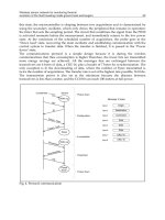
Figure 3 shows the process of metrics computing in member nodes. This node manages
functions such as capturing, sending and receiving data messages, in addition to the functions
of calculation of a security metrics like: the number of incoming and outgoing packet in a time
interval, number of dropped packets, etc. Among the population of member nodes in the
cluster, one representative sample of the population is chosen randomly. This sample will be
analyzed in the period of ongoing monitoring. Each node in a chosen sample performs a
calculation of his status. Once a difference in status between two time intervals is detected a
calculated indicators values of security will be sent to the cluster Head for analyses.


Fig. 3. Calculation of security metrics in each member node of a chosen sample

When sensor data are transmitted to the cluster head, nodes do not transmit sensor data if
their data are not changed since last reported. For example, at the current round, sensor
member S1 does not transmit its data to the cluster head because its data equal the collected
data at the next round.

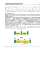
D. Local Monitoring in Cluster Head
The Cluster Head in figure 4, manages only the functions: self-monitoring of its state, local
monitoring of the results obtained from the member nodes of its cluster, the reception and
the emission of the messages, but does not manage, the function of capture of event. Cluster
head is good at making decision because it has both network-level information and host-

based information of all its nodes. The Cluster Head aggregates the results and send them to
the base station for more global analysis; this strategy reduces the number of alerts gone up
towards the base station.
 Cluster head can monitor its nodes thus to save their resources, or it can collect
monitoring report from nodes and do some additional work.
 Cluster head is good at making decision because it has both network-level
information and host-based information of all its nodes.


Fig. 4. Local Monitoring

E. Global Monitoring
The global observer receives the local traces collected by the local observers (the clusters-
head) in order to analyze them. The first step toward performing this analysis is to correlate
the traces and order them chronologically. In the network, all the nodes run with the same
clock value allowing thus to perform the trace correlation.

Fig. 5. Global Monitoring in Base Station
Sustainable Wireless Sensor Networks62

In First, the global observer collected alerts, have to be analyzed using a pre-processing
module that performs the following tasks:
- Filtering the collected alerts keeping only the relevant information.
- Alert correlation and the construction of a unique global trace file.
F. Distributed Monitoring based clustering architecture
Clustering facilitates the distribution of control over the network. Clustering saves energy
and reduces network contention by enabling locality of communication.

In our case, sensor networks are divided into cluster. The reorganization of the cluster will
be made for a security reason, where each cluster Head monitors the member nodes of their

cluster, which also facilitates the risen of alerts and reduces latency problems. These clusters
are generated automatically after an epoch of clusters formation. Every cluster is assigned a
cluster head CH, by election with some metrics. We opted for an election of cluster head
according a new metrics based on multiple criteria decision approach to decision support
for the selection of CHs, the criteria are: the criterion of density (the degree of connectivity of
each node), the criterion of energy (the level of residual energy in each node), the distance
between nodes in the cluster, the behavior level of each node and the index of mobility. Each
node calculates its metrics locally, then evaluates a function of weight according to these
metric (each node is limited to the closest neighbors), and diffuses the value of this function
to its neighbors. Cluster Head of each cluster is then elected of these results. Three
constraints which are the fact, that two CH cannot be coast at coast, and that if a node
belongs to two clusters, it must belong with the nearest cluster (by using a parameter of
distances), finally if a node is completely isolated it becomes automatically a cluster Head.

1) Clustering algorithm metric
We describe in this section, the metric used in our algorithm for clustering formation, then
we present its election protocol and update policy. The updating policy is locally called after
mobility or -adding new nodes in the network. To decide how much a node is suited for
being a cluster head to offer security services, we take into consideration the following
characteristics:

The node behaviour level B(i,t): Nodes with a behaviour level less than a threshold
behaviour-Min will not be accepted as candidate for being cluster heads even if they have
other interesting characteristics as high energy, high degree of connectivity or low mobility.
First of all each nodes are assigned a same static behaviour level B=1. However, this level
can be decreased by the anomaly detection algorithm if a nodes are misbehaving B=B – rate.
Classification of the behaviour value takes the following values:

Fig. 6. Behavior Level, B[0,1]

Classification of the behaviour value takes the following values:












3.00:
5.03.0:
8.05.0:malicious)not but (
18.0:
BNodeMalicious
BNodeSuspect
BNodeAbnormal
BNodeNormal
(5)


The node mobility M(i,t): We aim to have stable clusters. So, we should elect nodes with
low relative mobility as cluster heads. To characterize the instantaneous nodal mobility, we
will use a simple heuristic mechanism [71,72] where each node i estimates its relative
mobility index Mi by implementing the following procedure:

Compute the running average of the speed for every node i till current time T. This gives a
measure of mobility and is denoted by M
i
, as:






T
t
tttti
yyxx
T
M
1
2
1
2
1
)()(
1
(6)

Where (x
t
, y
t
) and (x

t-1
, y
t-1
) are the coordinates of the node v at time t and (t -1) ,
respectively.

The distance to neighbors D(i,t): It is better to elect the node with the nearest members as a
cluster head [73,74].
For every node i, compute the sum of the distances, D
i
, with all its neighbors j , as :







)(
),(
iNj
i
jidistD
(7)

The node remaining energy E(i,t): We should elect nodes with high remaining battery power
as cluster heads. The radio spends E
Tx-elec
= E
Rx-elec

= E
elec
energy to run receiver and
transmitter electronics. Therefore the transmission cost to transfer k-bit message to a
distance d is given by the equation (8) [75]:



2
),( dkEkEdkE
ampelecTx

(8)

Where E
amp
is a required amplifier energy. Similarly, the receiving cost can be given by
equation (9) :
E
Rx elec
(k) = kE (9)

The node connectivity degree C(i,t):
N(i) is the neighbors of node i , defined as [52] :





ijVj

range
txjidistjiN


,
),(][

(10)


Monitoring of Wireless Sensor Networks 63

In First, the global observer collected alerts, have to be analyzed using a pre-processing
module that performs the following tasks:
- Filtering the collected alerts keeping only the relevant information.
- Alert correlation and the construction of a unique global trace file.
F. Distributed Monitoring based clustering architecture
Clustering facilitates the distribution of control over the network. Clustering saves energy
and reduces network contention by enabling locality of communication.

In our case, sensor networks are divided into cluster. The reorganization of the cluster will
be made for a security reason, where each cluster Head monitors the member nodes of their
cluster, which also facilitates the risen of alerts and reduces latency problems. These clusters
are generated automatically after an epoch of clusters formation. Every cluster is assigned a
cluster head CH, by election with some metrics. We opted for an election of cluster head
according a new metrics based on multiple criteria decision approach to decision support
for the selection of CHs, the criteria are: the criterion of density (the degree of connectivity of
each node), the criterion of energy (the level of residual energy in each node), the distance
between nodes in the cluster, the behavior level of each node and the index of mobility. Each
node calculates its metrics locally, then evaluates a function of weight according to these

metric (each node is limited to the closest neighbors), and diffuses the value of this function
to its neighbors. Cluster Head of each cluster is then elected of these results. Three
constraints which are the fact, that two CH cannot be coast at coast, and that if a node
belongs to two clusters, it must belong with the nearest cluster (by using a parameter of
distances), finally if a node is completely isolated it becomes automatically a cluster Head.

1) Clustering algorithm metric
We describe in this section, the metric used in our algorithm for clustering formation, then
we present its election protocol and update policy. The updating policy is locally called after
mobility or -adding new nodes in the network. To decide how much a node is suited for
being a cluster head to offer security services, we take into consideration the following
characteristics:

The node behaviour level B(i,t): Nodes with a behaviour level less than a threshold
behaviour-Min will not be accepted as candidate for being cluster heads even if they have
other interesting characteristics as high energy, high degree of connectivity or low mobility.
First of all each nodes are assigned a same static behaviour level B=1. However, this level
can be decreased by the anomaly detection algorithm if a nodes are misbehaving B=B – rate.
Classification of the behaviour value takes the following values:

Fig. 6. Behavior Level, B[0,1]



Classification of the behaviour value takes the following values:













3.00:
5.03.0:
8.05.0:malicious)not but (
18.0:
BNodeMalicious
BNodeSuspect
BNodeAbnormal
BNodeNormal
(5)


The node mobility M(i,t): We aim to have stable clusters. So, we should elect nodes with
low relative mobility as cluster heads. To characterize the instantaneous nodal mobility, we
will use a simple heuristic mechanism [71,72] where each node i estimates its relative
mobility index Mi by implementing the following procedure:
Compute the running average of the speed for every node i till current time T. This gives a
measure of mobility and is denoted by M
i
, as:







T
t
tttti
yyxx
T
M
1
2
1
2
1
)()(
1
(6)

Where (x
t
, y
t
) and (x
t-1
, y
t-1
) are the coordinates of the node v at time t and (t -1) ,
respectively.

The distance to neighbors D(i,t): It is better to elect the node with the nearest members as a
cluster head [73,74].

For every node i, compute the sum of the distances, D
i
, with all its neighbors j , as :







)(
),(
iNj
i
jidistD
(7)

The node remaining energy E(i,t): We should elect nodes with high remaining battery power
as cluster heads. The radio spends E
Tx-elec
= E
Rx-elec
= E
elec
energy to run receiver and
transmitter electronics. Therefore the transmission cost to transfer k-bit message to a
distance d is given by the equation (8) [75]:




2
),( dkEkEdkE
ampelecTx

(8)

Where E
amp
is a required amplifier energy. Similarly, the receiving cost can be given by
equation (9) :
E
Rx elec
(k) = kE (9)

The node connectivity degree C(i,t):
N(i) is the neighbors of node i , defined as [52] :





ijVj
range
txjidistjiN


,
),(][

(10)

Sustainable Wireless Sensor Networks64

Find the neighbors of each node i which defines its degree d
i
as :


 



ijVj
rangei
txjidistiNC
,
),()(

(11)

We should elect nodes with very high connectivity as cluster heads.
Each node S
i
computes its weight P
i
according to the method of weighted sum decision
model, given by equation (12) :

P

i
= w
1
*B
i
+ w
2
*Er
i
+ w
3
*M
i
+ w
4
*C
i
+ w
5
*D
i
(12)

where w
1
, w
2
, w
3
,w

4
,w
5
are the weighing factors for the corresponding system parameters, such
that (w
1
+w
2
+w
3
+w
4
+w
5
=10), and since our goal is to monitor sensor we taken a high coefficients
for the behavior B
i
and the remaining energy Er
i
, as follows: w
1
=4 , w
2
=3, w
3
=1, w
4
=1, w
5
=1.

2) Node Status
A node in wireless sensor network can be in one of the 3 possible states: MEMBER (ME),
HEAD (CH), Monitor Node or Guard node (MO). Initially, every node is in ME state. It
starts election and may become CH node if it does not have link to any CH node, otherwise
it still a member ME.
3) Proposed Methodology
Our goal is to detect malicious activities in the network caused by the attacks and the failure
of nodes. We will offer primarily an organization of cluster network, where the cluster- head
of each cluster is responsible for monitoring the member nodes of its cluster. Subsequently
we propose a system for detecting anomalies based on a distributed approach.

4.4 Simulation and Results
In this section, we present the simulation model and results of our work.

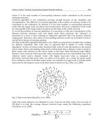
4.4.1 Simulation model
We developed a wireless sensor network simulator to create an environment to evaluate
our work. It is a discrete event simulator written in C++. A network generator was built,
which generates networks comprised of normal nodes plus malicious node, all located in
an square field. Each node has randomized x and y coordinates. No two different nodes
share the same coordinates. In our simulation, the sensor nodes are randomly distributed in
a 880mx360m square field, the communication range is 150m. The scenario simulation
consists of two steps: the first is for the formation of cluster, the second is to monitor the
network by different cluster head and the detection of the abnormal behaviour. For the
simulation of abnormal behaviour in the network, we generated a number of malicious
nodes that their state will move from a normal node with green colour to a abnormal node
with yellow colour, to a suspicious node of red colour , and lastly, a malicious node with
black colour. All the states of member nodes are detected by their cluster head. Malicious
cluster head are detected by the base station.

4.4.2 Results
In the following, we present and discuss the simulation results.

Fig. 7. Random deployment and graph connectivity of 100 nodes in square field.


Fig. 8. Network after Clustering Formation



Fig. 9. Sensors with yellow colour Fig. 10. the red sensors have a suspect
are abnormal but not malicious behaviour
Monitoring of Wireless Sensor Networks 65

Find the neighbors of each node i which defines its degree d
i
as :


 



ijVj
rangei
txjidistiNC
,
),()(

(11)

We should elect nodes with very high connectivity as cluster heads.
Each node S
i
computes its weight P
i
according to the method of weighted sum decision
model, given by equation (12) :

P
i
= w
1
*B
i
+ w
2
*Er
i
+ w
3
*M
i
+ w
4
*C
i
+ w
5

*D
i
(12)

where w
1
, w
2
, w
3
,w
4
,w
5
are the weighing factors for the corresponding system parameters, such
that (w
1
+w
2
+w
3
+w
4
+w
5
=10), and since our goal is to monitor sensor we taken a high coefficients
for the behavior B
i
and the remaining energy Er
i

, as follows: w
1
=4 , w
2
=3, w
3
=1, w
4
=1, w
5
=1.
2) Node Status
A node in wireless sensor network can be in one of the 3 possible states: MEMBER (ME),
HEAD (CH), Monitor Node or Guard node (MO). Initially, every node is in ME state. It
starts election and may become CH node if it does not have link to any CH node, otherwise
it still a member ME.
3) Proposed Methodology
Our goal is to detect malicious activities in the network caused by the attacks and the failure
of nodes. We will offer primarily an organization of cluster network, where the cluster- head
of each cluster is responsible for monitoring the member nodes of its cluster. Subsequently
we propose a system for detecting anomalies based on a distributed approach.

4.4 Simulation and Results
In this section, we present the simulation model and results of our work.

4.4.1 Simulation model
We developed a wireless sensor network simulator to create an environment to evaluate
our work. It is a discrete event simulator written in C++. A network generator was built,
which generates networks comprised of normal nodes plus malicious node, all located in
an square field. Each node has randomized x and y coordinates. No two different nodes

share the same coordinates. In our simulation, the sensor nodes are randomly distributed in
a 880mx360m square field, the communication range is 150m. The scenario simulation
consists of two steps: the first is for the formation of cluster, the second is to monitor the
network by different cluster head and the detection of the abnormal behaviour. For the
simulation of abnormal behaviour in the network, we generated a number of malicious
nodes that their state will move from a normal node with green colour to a abnormal node
with yellow colour, to a suspicious node of red colour , and lastly, a malicious node with
black colour. All the states of member nodes are detected by their cluster head. Malicious
cluster head are detected by the base station.



4.4.2 Results
In the following, we present and discuss the simulation results.

Fig. 7. Random deployment and graph connectivity of 100 nodes in square field.


Fig. 8. Network after Clustering Formation



Fig. 9. Sensors with yellow colour Fig. 10. the red sensors have a suspect
are abnormal but not malicious behaviour
Sustainable Wireless Sensor Networks66


Fig. 11. The sensors with black color are compromised and have an malicious behavior

The black sensors will be placed in a black list and will be disconnected from the network, as

shown in Figure 11.

5. Conclusion
In this chapter we started with the presentation of the overview of the mechanisms of
monitoring a wireless sensor networks, for the following reasons: topology control
(connectivity and the coverage), and the security in wireless sensor networks. Then we have
developed a new monitoring mechanism to guarantee strong connectivity in wireless
sensors networks, this mechanism is based on the distributed algorithms. The mechanism
monitors sensor connectivity and at any time is able to detect the critical nodes that
represent articulation points. Such articulation points are liable to cause portions of the
network to become disconnected and we have therefore also developed a mechanism for
self-organization to increase the degree of connectivity in their vicinity, by increasing fault
tolerance. Since connectivity is closely related to the coverage of targets, we have also
developed a way to monitor the robustness of the coverage between fixed targets and sensor
nodes. The main advantage of our approach is the ability to anticipate disconnections before
they occur. We are also able to reduce the number of monitoring node and assume
mechanisms for fault tolerance by auto organization of nodes to increase connectivity.
Finally, we have demonstrated the effectiveness of our approach and algorithms with
satisfactory results obtained through simulation.

After that we have presented our second contribution for the security of a wireless sensor
networks based on the distributed monitoring mechanisms. We have presented a
decentralized approach to monitor the status and behavior in a wireless sensor network. For
this we have developed a completed distributed monitoring mechanism for securing
wireless sensor networks. Based on a flexible weight clustering algorithm, a number of
parameters of nodes were taken into consideration for assigning weight to a node and
election cluster-head. The proposed algorithm chooses the robust cluster-heads who is the
responsibility to monitor a chosen sample of nodes in their cluster, and maintains clusters
locally. A second algorithm analyzes and detects a specific misbehavior in wireless sensor
networks. This algorithm insures the update of a behavior-level metric and isolates the

misbehaving node. The advantage of our approach is the minimization of the
communication between the monitor’s nodes and the normal nodes.

6. References
[1] I. F. Akyildiz, W. Su, Y. Sankarasubramaniam, E. Cyirci, "Wireless Sensor Networks: A
Survey.", Computer Networks, vol. 38, no.4, pp. 393-422, 2002.
[2] L. Kleinrock and J. Silvester. "Optimum transmission radio for packet radio networks or
why six is a magic number. In National Telecommunications Conference,
Birmingham, Alabama, pages 4.3.2–4.3.5, December 1978.
[3] A. Cerpa and D. Estrin, "Ascent: Adaptive self-configuring sensor networks topologies"
IEEE Transactions on Mobile Computing, vol. 3, no. 3, pp. 272–285, 2004.
[4] N. Li and J. C. Hou, "Improving connectivity of wireless ad hoc networks", in
MOBIQUITOUS ’05: Proceedings of the The Second Annual International
Conference on Mobile and Ubiquitous Systems: Networking and Services.
Washington, DC, USA: IEEE Computer Society, 2005, pp. 314–324.
[5] M. Dunbabin, P. Corke, I. Vasilescu, and D. Rus, "Data muling over underwater wireless
sensor networks using an autonomous underwater vehicle.", in IEEE International
Conference on Robotics and Automation (ICRA), 2006, May 15- 19 2006, pp. 2091–
2098.
[6] K. Benahmed, H. Haffaf , M. Merabti, D. Llewellyn-Jones, "Monitoring Connectivity in
Wireless Sensor Networks ", International Journal of Future Generation
Communication and Networking, Vol. 2, No. 2, 2009.
[7] G. Yang, L J. Chen, T. Sun, B. Zhou, and M. Gerla, "Ad-hoc storage overlay system
(asos): A delay-tolerant approach in manets.", in Proceeding of the IEEE MASS,
2006, pp. 296–305.
[8] N. Rao, W. Qishi, S. Iyengar, and A. Manickam, "Connectivity-through-time protocols for
dynamic wireless networks to support mobile robot teams.", in IEEE International
Conference on Robotics and Automation (ICRA), 2003, vol. 2, Sept 14-19 2003, pp.
1653–1658.

[9] D. Ganesan, R. Govindan, S. Shenker, and D. Estrin Highly-Resilient, "Energy-Efficient
Multipath Routing in Wireless Sensor Networks.", Mobile Computing and
Communications Review, 1(2), 1997.
[10] D. Spanos and R. Murray, "Motion planning with wireless network constraints.", in
Proceedings of the 2005 American Control Conference, 2005, pp. 87–92.
[11] D. Desovski, Y. Liu, and B. Cukic. "Linear randomized voting algorithm for fault
tolerant sensor fusion and the corresponding reliability model.", In IEEE
International Symposium on Systems Engineering, pages 153–162, October 2005.
[12] A. Boukerche, "Handbook of Algorithms and Protocols for Wireless and Mobile
Networks", Chapman CRC/Hall, 2005.
[13] N. Li and J. C. Hou. "FLSS: A Fault-Tolerant Topology Control Algorithm for Wireless
Networks.", In Proceedings of the 10th Annual International Conference on Mobile
Computing and Networking, pages 275–286, 2004.
Monitoring of Wireless Sensor Networks 67


Fig. 11. The sensors with black color are compromised and have an malicious behavior

The black sensors will be placed in a black list and will be disconnected from the network, as
shown in Figure 11.

5. Conclusion
In this chapter we started with the presentation of the overview of the mechanisms of
monitoring a wireless sensor networks, for the following reasons: topology control
(connectivity and the coverage), and the security in wireless sensor networks. Then we have
developed a new monitoring mechanism to guarantee strong connectivity in wireless
sensors networks, this mechanism is based on the distributed algorithms. The mechanism
monitors sensor connectivity and at any time is able to detect the critical nodes that
represent articulation points. Such articulation points are liable to cause portions of the
network to become disconnected and we have therefore also developed a mechanism for

self-organization to increase the degree of connectivity in their vicinity, by increasing fault
tolerance. Since connectivity is closely related to the coverage of targets, we have also
developed a way to monitor the robustness of the coverage between fixed targets and sensor
nodes. The main advantage of our approach is the ability to anticipate disconnections before
they occur. We are also able to reduce the number of monitoring node and assume
mechanisms for fault tolerance by auto organization of nodes to increase connectivity.
Finally, we have demonstrated the effectiveness of our approach and algorithms with
satisfactory results obtained through simulation.

After that we have presented our second contribution for the security of a wireless sensor
networks based on the distributed monitoring mechanisms. We have presented a
decentralized approach to monitor the status and behavior in a wireless sensor network. For
this we have developed a completed distributed monitoring mechanism for securing
wireless sensor networks. Based on a flexible weight clustering algorithm, a number of
parameters of nodes were taken into consideration for assigning weight to a node and
election cluster-head. The proposed algorithm chooses the robust cluster-heads who is the
responsibility to monitor a chosen sample of nodes in their cluster, and maintains clusters
locally. A second algorithm analyzes and detects a specific misbehavior in wireless sensor
networks. This algorithm insures the update of a behavior-level metric and isolates the

misbehaving node. The advantage of our approach is the minimization of the
communication between the monitor’s nodes and the normal nodes.

6. References
[1] I. F. Akyildiz, W. Su, Y. Sankarasubramaniam, E. Cyirci, "Wireless Sensor Networks: A
Survey.", Computer Networks, vol. 38, no.4, pp. 393-422, 2002.
[2] L. Kleinrock and J. Silvester. "Optimum transmission radio for packet radio networks or
why six is a magic number. In National Telecommunications Conference,
Birmingham, Alabama, pages 4.3.2–4.3.5, December 1978.
[3] A. Cerpa and D. Estrin, "Ascent: Adaptive self-configuring sensor networks topologies"

IEEE Transactions on Mobile Computing, vol. 3, no. 3, pp. 272–285, 2004.
[4] N. Li and J. C. Hou, "Improving connectivity of wireless ad hoc networks", in
MOBIQUITOUS ’05: Proceedings of the The Second Annual International
Conference on Mobile and Ubiquitous Systems: Networking and Services.
Washington, DC, USA: IEEE Computer Society, 2005, pp. 314–324.
[5] M. Dunbabin, P. Corke, I. Vasilescu, and D. Rus, "Data muling over underwater wireless
sensor networks using an autonomous underwater vehicle.", in IEEE International
Conference on Robotics and Automation (ICRA), 2006, May 15- 19 2006, pp. 2091–
2098.
[6] K. Benahmed, H. Haffaf , M. Merabti, D. Llewellyn-Jones, "Monitoring Connectivity in
Wireless Sensor Networks ", International Journal of Future Generation
Communication and Networking, Vol. 2, No. 2, 2009.
[7] G. Yang, L J. Chen, T. Sun, B. Zhou, and M. Gerla, "Ad-hoc storage overlay system
(asos): A delay-tolerant approach in manets.", in Proceeding of the IEEE MASS,
2006, pp. 296–305.
[8] N. Rao, W. Qishi, S. Iyengar, and A. Manickam, "Connectivity-through-time protocols for
dynamic wireless networks to support mobile robot teams.", in IEEE International
Conference on Robotics and Automation (ICRA), 2003, vol. 2, Sept 14-19 2003, pp.
1653–1658.
[9] D. Ganesan, R. Govindan, S. Shenker, and D. Estrin Highly-Resilient, "Energy-Efficient
Multipath Routing in Wireless Sensor Networks.", Mobile Computing and
Communications Review, 1(2), 1997.
[10] D. Spanos and R. Murray, "Motion planning with wireless network constraints.", in
Proceedings of the 2005 American Control Conference, 2005, pp. 87–92.
[11] D. Desovski, Y. Liu, and B. Cukic. "Linear randomized voting algorithm for fault
tolerant sensor fusion and the corresponding reliability model.", In IEEE
International Symposium on Systems Engineering, pages 153–162, October 2005.
[12] A. Boukerche, "Handbook of Algorithms and Protocols for Wireless and Mobile
Networks", Chapman CRC/Hall, 2005.
[13] N. Li and J. C. Hou. "FLSS: A Fault-Tolerant Topology Control Algorithm for Wireless

Networks.", In Proceedings of the 10th Annual International Conference on Mobile
Computing and Networking, pages 275–286, 2004.
Sustainable Wireless Sensor Networks68

[14] J. L. Bredin, E. D. Demaine, M. Hajiaghayi, and D. Rus. "Deploying Sensor Networks
with Guaranteed Capacity and Fault Tolerance.", In Proceedings of the 6th ACM
international symposium on Mobile ad hoc networking and computing, pages 309–
319, 2005.
[15] Bahramgiri, M., Hajiaghayi, M., and Mirrokni, "Fault-tolerant and 3-dimensional
distributed topology control algorithms in wireless multi-hop networks.", 2002.
[16] N. Li, J. Hou, and L. Sha. "Design and analysis of an mst-based topology control
algorithm." , In Proceedings of the IEEE INFOCOM, 2003.
[17] Xiang-Yang Li, Peng-Jun Wan, Yu Wang, and Chih-Wei Yi. "Fault tolerant deployment
and topology control in wireless networks.", In Proceedings of the 4th ACM
international symposium on Mobile ad hoc networking & computing (MobiHoc),
pages 117.128, 2003.
[18] Michaël Hauspie , "Contributions à l'étude des gestionnaires de services distribués dans
les réseaux ad hoc ", Thèse de doctorat, Université des Sciences et Technologies de
Lille, 2005.
[19] Bruno Courcelle, " Introduction à la théorie des graphes: Définitions, applications et
techniques de preuves ", Université Bordeaux 1, LaBRI (CNRS UMR 5800), 20
Avril, 2004.
[20] R. Tarjan., "Depth First Search and linear graph algorithms.", SIAM Journal of
Computing, 1:146_160, 1972.
[21] Wies law Zielonka , "Algorithmique ", LIAFA, Université Denis Diderot, Septembre
2006.
[22] K. Chakrabarty, S. S. Iyengar, H. Qi, E. Cho, "Grid coverage for surveillance and target
location in distributed sensor networks," IEEE Transactions on Computers,
51(12):1448-1453, December 2002.
[23 ]S. Meguerdichian and M. Potkonjak. "Low Power 0/1 Coverage and Scheduling

Techniques in Sensor Networks." UCLA Technical Reports 030001. January 2003.
[24]S. Meguerdichian, F. Koushanfar, M. Potkonjak, and M. Srivastava, "Coverage Problems
in Wireless Ad-Hoc Sensor Networks." IEEE Infocom 2001, Vol 3, pp. 1380-1387,
April 2001.
[25] S. Meguerdichian, F. Koushanfar, G. Qu, and M. Potkonjak, "Exposure in Wireless Ad
Hoc Sensor Networks." Procs. of 7th Annual International Conference on Mobile
Computing and Networking (MobiCom'01), pp. 139-150, July 2001.
[26] T. Couqueur, V. Phipatanasuphorn, P. Ramanathan and K. K. Saluja, "Sensor
Deployment Strategy for Target Detection," Proceeding of The First ACM
International Workshop on Wireless Sensor Networks and Applications, Sep. 2002.
[27] D. Tian and N.D. Georganas, "A Coverage-preserved Node Scheduling scheme for
Large Wireless Sensor Networks," Proceedings of First International Workshop on
Wireless Sensor Networks and Applications (WSNA'02), Atlanta, USA, September
2002.
[28] A. Cerpa and D. Estrin, "ASCENT: Adaptive Self-Configuring Sensor Networks
Topologies," International Annual Joint Conference of the IEEE Computer and
Communications Societies (INFOCOM 2002), New York, NY, USA, June 23-27 2002.

[29] B. Chen, K. Jamieson, H. Balakrishnan, and R. Morris, "Span: An Energy-Efficient
Coordination Algorithm for Topology Maintenance in Ad Hoc Wireless Networks,"
ACM/IEEE International Conference on Mobile Computing and Networking
(MobiCom 2001), Rome, Italy, July 16-21, 2001.
[30] Y. Xu, J. Heidemann, and D. Estrin, "Adaptive Energy-Conserving Routing for
Multihop Ad Hoc Networks," Research Report 527, USC/Information Sciences
Institute, October 2000.
[31] Y. Xu, J. Heidemann, and D. Estrin, "Geography-informed Energy Conservation for Ad
Hoc Routing," ACM/IEEE International Conference on Mobile Computing and
Networking (MobiCom 2001), Rome, Italy, July 16-21, 2001.
[32] F. Ye, G. Zhong, S. Lu, and L. Zhang, "PEAS: A Robust Energy Conserving Protocol for
Long-lived Sensor Networks". The 23rd International Conference on Distributed

Computing Systems (ICDCS'03), May 2003.
[33] A. Perrig, "SPINS: security protocols for sensor networks," In Proc. of ACM MobiCom,
2001.
[34] S. Ganeriwal and M. B. Srivastava, "Reputation-based framework for high integrity
sensor networks," In Proc. Of ACM SASN, 2004.
[35] I. Khalil, S. Bagchi, and C. Nina-Rotaru, "DICAS: detection, diagnosis and isolation of
control attacks in sensor networks," In Proc. of IEEE SecureComm, 2005.
[36] S B. Lee and Y H. Choi, "A resilient packet-forwarding scheme against maliciously
packet-dropping nodes in sensor networks," In Proc. of ACM SASN, 2006.
[37] I. Khalil, S. Bagchi, and N. Shroff, "LITEWORP: a lightweight countermeasure for the
wormhole attack in multihop wireless networks," In Proc. of IEEE/IFIP DSN, 2005.
[38] S. Ganeriwal and M. B. Srivastava, "Reputation-based framework for high integrity
sensor networks," In Proc. Of ACM SASN, 2004.
[39] [S. Buchegger and J Y. L. Boudec, "Performance analysis of the CONFIDANT protocol:
cooperation of nodes fairness in distributed ad-hoc networks," In Proc. of ACM
MobiHoc, 2002.
[40] P. Michiardi and R. Molva, "CORE: a collaborativereputation mechanism to enforce
node cooperation in mobile ad hoc networks," In Proc. of the IFIP Sixth Joint
Working Conference on Communications and Multimedia Security, 2002
[41] K. Ioannis, T. Dimitriou, and F. C. Freiling, "Towards intrusion detection in wireless
sensor networks," In Proc. of the 13th European Wireless Conference, 2007.
[42] Y. Huang and W. Lee, "A cooperative intrusion detection system for ad hoc networks,"
In Proc. of ACM SASN, 2003.
[43] I. Khalil, S. Bagchi, and N. B. Shroff, "SLAM: sleep-wake aware local monitoring in
sensor networks," In Proc. Of IEEE/IFIP DSN, 2007.
[44] C. Hsin and M. Liu, "Self-monitoring of wireless sensor networks," Elsevier Computer
Communications, vol. 29, pp.462-476, 2006.
[45] T. H. Hai1, E N. Huh, and M. Jo,“A lightweight intrusion detection framework for
wireless sensor networks”, Wirel. Commun. Mob. Comput. (2009)
[46] Q. Wang, T. Zhang , “Detecting Anomaly Node Behavior in Wireless Sensor Networks”,

21st International Conference on Advanced Information Networking and
Applications Workshops, 2007.
Monitoring of Wireless Sensor Networks 69

[14] J. L. Bredin, E. D. Demaine, M. Hajiaghayi, and D. Rus. "Deploying Sensor Networks
with Guaranteed Capacity and Fault Tolerance.", In Proceedings of the 6th ACM
international symposium on Mobile ad hoc networking and computing, pages 309–
319, 2005.
[15] Bahramgiri, M., Hajiaghayi, M., and Mirrokni, "Fault-tolerant and 3-dimensional
distributed topology control algorithms in wireless multi-hop networks.", 2002.
[16] N. Li, J. Hou, and L. Sha. "Design and analysis of an mst-based topology control
algorithm." , In Proceedings of the IEEE INFOCOM, 2003.
[17] Xiang-Yang Li, Peng-Jun Wan, Yu Wang, and Chih-Wei Yi. "Fault tolerant deployment
and topology control in wireless networks.", In Proceedings of the 4th ACM
international symposium on Mobile ad hoc networking & computing (MobiHoc),
pages 117.128, 2003.
[18] Michaël Hauspie , "Contributions à l'étude des gestionnaires de services distribués dans
les réseaux ad hoc ", Thèse de doctorat, Université des Sciences et Technologies de
Lille, 2005.
[19] Bruno Courcelle, " Introduction à la théorie des graphes: Définitions, applications et
techniques de preuves ", Université Bordeaux 1, LaBRI (CNRS UMR 5800), 20
Avril, 2004.
[20] R. Tarjan., "Depth First Search and linear graph algorithms.", SIAM Journal of
Computing, 1:146_160, 1972.
[21] Wies law Zielonka , "Algorithmique ", LIAFA, Université Denis Diderot, Septembre
2006.
[22] K. Chakrabarty, S. S. Iyengar, H. Qi, E. Cho, "Grid coverage for surveillance and target
location in distributed sensor networks," IEEE Transactions on Computers,
51(12):1448-1453, December 2002.
[23 ]S. Meguerdichian and M. Potkonjak. "Low Power 0/1 Coverage and Scheduling

Techniques in Sensor Networks." UCLA Technical Reports 030001. January 2003.
[24]S. Meguerdichian, F. Koushanfar, M. Potkonjak, and M. Srivastava, "Coverage Problems
in Wireless Ad-Hoc Sensor Networks." IEEE Infocom 2001, Vol 3, pp. 1380-1387,
April 2001.
[25] S. Meguerdichian, F. Koushanfar, G. Qu, and M. Potkonjak, "Exposure in Wireless Ad
Hoc Sensor Networks." Procs. of 7th Annual International Conference on Mobile
Computing and Networking (MobiCom'01), pp. 139-150, July 2001.
[26] T. Couqueur, V. Phipatanasuphorn, P. Ramanathan and K. K. Saluja, "Sensor
Deployment Strategy for Target Detection," Proceeding of The First ACM
International Workshop on Wireless Sensor Networks and Applications, Sep. 2002.
[27] D. Tian and N.D. Georganas, "A Coverage-preserved Node Scheduling scheme for
Large Wireless Sensor Networks," Proceedings of First International Workshop on
Wireless Sensor Networks and Applications (WSNA'02), Atlanta, USA, September
2002.
[28] A. Cerpa and D. Estrin, "ASCENT: Adaptive Self-Configuring Sensor Networks
Topologies," International Annual Joint Conference of the IEEE Computer and
Communications Societies (INFOCOM 2002), New York, NY, USA, June 23-27 2002.

[29] B. Chen, K. Jamieson, H. Balakrishnan, and R. Morris, "Span: An Energy-Efficient
Coordination Algorithm for Topology Maintenance in Ad Hoc Wireless Networks,"
ACM/IEEE International Conference on Mobile Computing and Networking
(MobiCom 2001), Rome, Italy, July 16-21, 2001.
[30] Y. Xu, J. Heidemann, and D. Estrin, "Adaptive Energy-Conserving Routing for
Multihop Ad Hoc Networks," Research Report 527, USC/Information Sciences
Institute, October 2000.
[31] Y. Xu, J. Heidemann, and D. Estrin, "Geography-informed Energy Conservation for Ad
Hoc Routing," ACM/IEEE International Conference on Mobile Computing and
Networking (MobiCom 2001), Rome, Italy, July 16-21, 2001.
[32] F. Ye, G. Zhong, S. Lu, and L. Zhang, "PEAS: A Robust Energy Conserving Protocol for
Long-lived Sensor Networks". The 23rd International Conference on Distributed

Computing Systems (ICDCS'03), May 2003.
[33] A. Perrig, "SPINS: security protocols for sensor networks," In Proc. of ACM MobiCom,
2001.
[34] S. Ganeriwal and M. B. Srivastava, "Reputation-based framework for high integrity
sensor networks," In Proc. Of ACM SASN, 2004.
[35] I. Khalil, S. Bagchi, and C. Nina-Rotaru, "DICAS: detection, diagnosis and isolation of
control attacks in sensor networks," In Proc. of IEEE SecureComm, 2005.
[36] S B. Lee and Y H. Choi, "A resilient packet-forwarding scheme against maliciously
packet-dropping nodes in sensor networks," In Proc. of ACM SASN, 2006.
[37] I. Khalil, S. Bagchi, and N. Shroff, "LITEWORP: a lightweight countermeasure for the
wormhole attack in multihop wireless networks," In Proc. of IEEE/IFIP DSN, 2005.
[38] S. Ganeriwal and M. B. Srivastava, "Reputation-based framework for high integrity
sensor networks," In Proc. Of ACM SASN, 2004.
[39] [S. Buchegger and J Y. L. Boudec, "Performance analysis of the CONFIDANT protocol:
cooperation of nodes fairness in distributed ad-hoc networks," In Proc. of ACM
MobiHoc, 2002.
[40] P. Michiardi and R. Molva, "CORE: a collaborativereputation mechanism to enforce
node cooperation in mobile ad hoc networks," In Proc. of the IFIP Sixth Joint
Working Conference on Communications and Multimedia Security, 2002
[41] K. Ioannis, T. Dimitriou, and F. C. Freiling, "Towards intrusion detection in wireless
sensor networks," In Proc. of the 13th European Wireless Conference, 2007.
[42] Y. Huang and W. Lee, "A cooperative intrusion detection system for ad hoc networks,"
In Proc. of ACM SASN, 2003.
[43] I. Khalil, S. Bagchi, and N. B. Shroff, "SLAM: sleep-wake aware local monitoring in
sensor networks," In Proc. Of IEEE/IFIP DSN, 2007.
[44] C. Hsin and M. Liu, "Self-monitoring of wireless sensor networks," Elsevier Computer
Communications, vol. 29, pp.462-476, 2006.
[45] T. H. Hai1, E N. Huh, and M. Jo,“A lightweight intrusion detection framework for
wireless sensor networks”, Wirel. Commun. Mob. Comput. (2009)
[46] Q. Wang, T. Zhang , “Detecting Anomaly Node Behavior in Wireless Sensor Networks”,

21st International Conference on Advanced Information Networking and
Applications Workshops, 2007.
Sustainable Wireless Sensor Networks70

[47] K. Ramachandran, E. M. Belding-Royer, and K. C. Almeroth. DAMON: A Distributed
Architecture for Monitoring Multi-hop Mobile Networks. In Proceedings of the 1st
IEEE International Conference on Sensor and Ad hoc Communications and
Networks (SECON), October 2004.
[48] J. Zhao, R. Govindan, and D. Estrin. Residual energy scans for monitoring wireless
sensor networks. In IEEE Wireless Communications and Networking Conference
(WCNC), 2002.
[49] NIthya Ramanathan, Kevin Chang, Rahul Kapur, Lewis Girod, Eddie Kohler, Deborah
Estrin. Sympathy for the Sensor Network Debugger. In 3rd Embedded networked
sensor systems. 2005. San Diego, USA: ACM Press.
[50] Y. an Huang and W. Lee, A cooperative intrusion detection system for ad hoc networks,
in Proc of the 1st ACM Workshop on Security of Ad hoc and Sensor Networks,
2003, pp. 135–147.
[51] S. Marti, T. J. Giuli, K. Lai, and M. Baker, Mitigating routing misbehavior in mobile ad
hoc networks, in Mobile Computing and Networking, 2000, pp. 255–265.
[52] K. Benahmed, H. Haffaf, M. Merabti, D. Llewellyn-Jones, "Monitoring connectivity in
Wireless Sensor Networks", IEEE Symposium on Computers and Communications
(ISCC'09), Sousse, Tunisia, 5-8 July 2009.
[53] Tanya Roosta, Shiuhpyng Winston Shieh, S. Shankar Sastry. "Taxonomy of Security
Attacks in Sensor Networks and Countermeasures ". The First IEEE International
Conference on System Integration and Reliability Improvements, December, 2006.
[54] T.Kavitha, D.Sridharan, “Security Vulnerabilities In Wireless Sensor Networks: A
Survey”, Journal of Information Assurance and Security 5 (2010) 031-044
[55] Song Han, Elizabeth Chang, Li Gao and Tharam Dillon, "Taxonomy of Attacks on
Wireless Sensor Networks", Proceedings of the First European Conference on
Computer Network Defence School of Computing, University of Glamorgan,

Wales, UK, 2005.
[56] M.Yu, H.Mokhtar, M.Merabti,"A Survey on Fault Management in Wireless Sensor
Networks", School of Computing & Mathematical Science Liverpool John Moores
University. UK, 2007.
[57] Chihfan Hsin, Mingyan Liu. A Distributed Monitoring Mechanism for Wireless Sensor
Networks. in 3rd workshopo on Wireless Security. 2002: ACM Press.
[58] Jinran Chen, Shubha Kher, Arun Somani. Distributed Fault Detection of Wireless Sensor
Networks. in DIWANS'06. 2006. Los Angeles, USA: ACM Pres.
[59] Anmol Sheth, Carl Hartung, Richard Han. A Decentralized Fault Diagnosis System for
Wireless Sensor Networks. in 2nd Mobile Ad Hoc and Sensor Systems. 2005.
Washington, USA.
[60] Sergio Marti, T.J.Giuli, Kevin Lai, Mary Baker. Mitigating Routing Misbehavior in
Mobile Ad Hoc Networks. in 6th International Conference on Mobile Computing
and Networking. 2000. Boston, Massachusetts, USA: ACM.
[61] Y. Huang and W. Lee, “A cooperative intrusion detection system for ad hoc networks,”
in Proceedings of the 1st ACM workshop on Security of ad hoc and sensor
networks, pp. 135-147, 2003.

[62] A. Silva, M. Martins, B. Rocha, A. Loureiro, L. Ruiz, and H. Wong, “Decentralized
intrusion detection in wireless sensor networks,” in Proceedings of the 1st ACM
international workshop on Quality of service & security in wireless and mobile
networks, pp. 16-23, 2005.
[63] M. Saraogi, “security in wireless sensor networks” , University of Tennessee, 2005.
[64] J.P. Mäkelä, “Security in Wireless Sensor Networks”, Oulu University of Applied
Sciences, School of Engineering, Oulu, Finland, 2009.
[65] J. Rehana, "Security of Wireless Sensor Network" Helsinki University of Technology,
Helsinki, Technical Report TKK-CSE-B5, 2009.
[66] I. Chatzigiannakis, ”A Decentralized Intrusion Detection System for Increasing Security
of Wireless Sensor Networks”, University of Patras, Greece, 2007.
[67] C. Karlof, D. Wagner, “Secure routing in wireless sensor networks: Attacks and

countermeasures”. In Proceedings of the 1st IEEE International Workshop on
Sensor Network Protocols and Applications (Anchorage, AK, May 11, 2003).
[68] Al-Sakib Khan Pathan, Hyung-Woo Lee, Choong Seon Hong, “Security in Wireless
Sensor Networks: Issues and Challenges”, Proceedings of 8th IEEE ICACT 2006,
Volume II, February 20-22, Phoenix Park, Korea, 2006, pp. 1043-1048.
[69] John Paul Walters, Zhengqiang Liang, Weisong Shi, and Vipin Chaudhary ,“Wireless
Sensor Network Security: A Survey”, in Distributed, Grid, and Pervasive
Computing, Yang Xiao (Eds.), 2006.
[70] E. Z. Ang, "Node Misbehaviour in Mobile Ad Hoc Networks," National University of
Singapore, 2004.
[71] A. H. Hussein, A. O. Abu Salem, S. Yousef ,“A Flexible Weighted Clustering Algorithm
Based on Battery Power for Mobile Ad Hoc Networks”, IEEE, 2008.
[72] C. Li, Y Wang, F. Huang, D. Yang,“ A Novel Enhanced Weighted Clustering Algorithm
for Mobile Networks”, IEEE 2009.
[73] B. Kadri, A. M’hamed, M. Feham , “Secured Clustering Algorithm for Mobile Ad Hoc
Networks”, IJCSNS , VOL.7 No.3, March 2007.
[74] M. Chatterjee, S. K. DAS, D. Turgut, “WCA: A Weighted Clustering Algorithm for
Mobile Ad Hoc Networks”, Cluster Computing 5, 193–204, 2002.
[75] Z. J wu, J. Y ying, Z. J ji, Y. C lei,“A Weighted Clustering Algorithm Based Routing
Protocol in Wireless Sensor Networks ”, ISECS 2008.



Monitoring of Wireless Sensor Networks 71

[47] K. Ramachandran, E. M. Belding-Royer, and K. C. Almeroth. DAMON: A Distributed
Architecture for Monitoring Multi-hop Mobile Networks. In Proceedings of the 1st
IEEE International Conference on Sensor and Ad hoc Communications and
Networks (SECON), October 2004.
[48] J. Zhao, R. Govindan, and D. Estrin. Residual energy scans for monitoring wireless

sensor networks. In IEEE Wireless Communications and Networking Conference
(WCNC), 2002.
[49] NIthya Ramanathan, Kevin Chang, Rahul Kapur, Lewis Girod, Eddie Kohler, Deborah
Estrin. Sympathy for the Sensor Network Debugger. In 3rd Embedded networked
sensor systems. 2005. San Diego, USA: ACM Press.
[50] Y. an Huang and W. Lee, A cooperative intrusion detection system for ad hoc networks,
in Proc of the 1st ACM Workshop on Security of Ad hoc and Sensor Networks,
2003, pp. 135–147.
[51] S. Marti, T. J. Giuli, K. Lai, and M. Baker, Mitigating routing misbehavior in mobile ad
hoc networks, in Mobile Computing and Networking, 2000, pp. 255–265.
[52] K. Benahmed, H. Haffaf, M. Merabti, D. Llewellyn-Jones, "Monitoring connectivity in
Wireless Sensor Networks", IEEE Symposium on Computers and Communications
(ISCC'09), Sousse, Tunisia, 5-8 July 2009.
[53] Tanya Roosta, Shiuhpyng Winston Shieh, S. Shankar Sastry. "Taxonomy of Security
Attacks in Sensor Networks and Countermeasures ". The First IEEE International
Conference on System Integration and Reliability Improvements, December, 2006.
[54] T.Kavitha, D.Sridharan, “Security Vulnerabilities In Wireless Sensor Networks: A
Survey”, Journal of Information Assurance and Security 5 (2010) 031-044
[55] Song Han, Elizabeth Chang, Li Gao and Tharam Dillon, "Taxonomy of Attacks on
Wireless Sensor Networks", Proceedings of the First European Conference on
Computer Network Defence School of Computing, University of Glamorgan,
Wales, UK, 2005.
[56] M.Yu, H.Mokhtar, M.Merabti,"A Survey on Fault Management in Wireless Sensor
Networks", School of Computing & Mathematical Science Liverpool John Moores
University. UK, 2007.
[57] Chihfan Hsin, Mingyan Liu. A Distributed Monitoring Mechanism for Wireless Sensor
Networks. in 3rd workshopo on Wireless Security. 2002: ACM Press.
[58] Jinran Chen, Shubha Kher, Arun Somani. Distributed Fault Detection of Wireless Sensor
Networks. in DIWANS'06. 2006. Los Angeles, USA: ACM Pres.
[59] Anmol Sheth, Carl Hartung, Richard Han. A Decentralized Fault Diagnosis System for

Wireless Sensor Networks. in 2nd Mobile Ad Hoc and Sensor Systems. 2005.
Washington, USA.
[60] Sergio Marti, T.J.Giuli, Kevin Lai, Mary Baker. Mitigating Routing Misbehavior in
Mobile Ad Hoc Networks. in 6th International Conference on Mobile Computing
and Networking. 2000. Boston, Massachusetts, USA: ACM.
[61] Y. Huang and W. Lee, “A cooperative intrusion detection system for ad hoc networks,”
in Proceedings of the 1st ACM workshop on Security of ad hoc and sensor
networks, pp. 135-147, 2003.

[62] A. Silva, M. Martins, B. Rocha, A. Loureiro, L. Ruiz, and H. Wong, “Decentralized
intrusion detection in wireless sensor networks,” in Proceedings of the 1st ACM
international workshop on Quality of service & security in wireless and mobile
networks, pp. 16-23, 2005.
[63] M. Saraogi, “security in wireless sensor networks” , University of Tennessee, 2005.
[64] J.P. Mäkelä, “Security in Wireless Sensor Networks”, Oulu University of Applied
Sciences, School of Engineering, Oulu, Finland, 2009.
[65] J. Rehana, "Security of Wireless Sensor Network" Helsinki University of Technology,
Helsinki, Technical Report TKK-CSE-B5, 2009.
[66] I. Chatzigiannakis, ”A Decentralized Intrusion Detection System for Increasing Security
of Wireless Sensor Networks”, University of Patras, Greece, 2007.
[67] C. Karlof, D. Wagner, “Secure routing in wireless sensor networks: Attacks and
countermeasures”. In Proceedings of the 1st IEEE International Workshop on
Sensor Network Protocols and Applications (Anchorage, AK, May 11, 2003).
[68] Al-Sakib Khan Pathan, Hyung-Woo Lee, Choong Seon Hong, “Security in Wireless
Sensor Networks: Issues and Challenges”, Proceedings of 8th IEEE ICACT 2006,
Volume II, February 20-22, Phoenix Park, Korea, 2006, pp. 1043-1048.
[69] John Paul Walters, Zhengqiang Liang, Weisong Shi, and Vipin Chaudhary ,“Wireless
Sensor Network Security: A Survey”, in Distributed, Grid, and Pervasive
Computing, Yang Xiao (Eds.), 2006.
[70] E. Z. Ang, "Node Misbehaviour in Mobile Ad Hoc Networks," National University of

Singapore, 2004.
[71] A. H. Hussein, A. O. Abu Salem, S. Yousef ,“A Flexible Weighted Clustering Algorithm
Based on Battery Power for Mobile Ad Hoc Networks”, IEEE, 2008.
[72] C. Li, Y Wang, F. Huang, D. Yang,“ A Novel Enhanced Weighted Clustering Algorithm
for Mobile Networks”, IEEE 2009.
[73] B. Kadri, A. M’hamed, M. Feham , “Secured Clustering Algorithm for Mobile Ad Hoc
Networks”, IJCSNS , VOL.7 No.3, March 2007.
[74] M. Chatterjee, S. K. DAS, D. Turgut, “WCA: A Weighted Clustering Algorithm for
Mobile Ad Hoc Networks”, Cluster Computing 5, 193–204, 2002.
[75] Z. J wu, J. Y ying, Z. J ji, Y. C lei,“A Weighted Clustering Algorithm Based Routing
Protocol in Wireless Sensor Networks ”, ISECS 2008.




Chapter title
Author Name
Part 2

Communications and Networking

Diversity Techniques for Robustness and Power Awareness
in Wireless Sensor Systems for Railroad Transport Applications 75
Diversity Techniques for Robustness and Power Awareness in Wireless
Sensor Systems for Railroad Transport Applications
Mathias Grudén, Magnus Jobs and Anders Rydberg
X

Diversity Techniques for Robustness and
Power Awareness in Wireless Sensor Systems

for Railroad Transport Applications

Mathias Grudén, Magnus Jobs and Anders Rydberg
Uppsala University
Sweden

1. Introduction
During the last decades business and industry has been constantly optimizing time in
production and transportation. This implies that the margins when doing business are
decreasing and when margins are decreasing more information is necessary so that the right
decisions can be made on time. This is especially important for the transport sector; in all
production there is a need to know when the freight with the components is arriving so that
the work can be planned. But as the system grows more sensitive to delays it also implies
that delays are getting very expensive. The transport of goods on e.g. trains has therefore to
be monitored carefully in order to retrieve information on delays. Theses delays can be
either due to normal circumstances occurring in transports such as scheduling of time tables
or due to mechanical faults. Ball bearings used in the trains are vulnerable to damage which
also stands for a large fraction of the mechanical faults that contribute to transport delays by
causing costly emergent stops.
Recently the Swedish Transport Administration evaluated a system for monitoring the
temperature of the ball bearings (Gruden M., et al, 2009). The evaluation was performed
within the Uppsala VINN Excellence Center for Wireless Sensor Networks (WISENET). The
evaluation was performed during 2008 by mounting wireless temperature sensors on the
ball bearings and with a wireless gateway onboard the train. The positions of the sensors
can be seen in Fig. 1.1. This system was monitoring the ball bearing of the wheels and air
temperature. The measured temperature of the ball bearing was continuously presented on
a webpage. By monitoring the temperature it is possible to see trends of heating and predict
if the train wagon needs maintenance or not. This type of monitoring system can greatly
increase the reliability of the overall system.
One problem noticed with this system onboard the train was the wireless robustness. Due to

the metal parts the wireless connection was partially intermittent. One technique which can
be used to improve the robustness of a system is the use of multiple antennas at the receiver
or transmitter. As the received signal might suffer severe variation from fading phenomena,
techniques must the implemented to mitigate these effects. The choice of techniques can
generally be classified into two parts, hardware and software. Software solutions to the
fading phenomena usually involve various coding techniques to improve the reliability but
4
Sustainable Wireless Sensor Networks76


this causes slower data rates. Hardware solutions can be found using diversity techniques
where two or more antennas are used and then combining the signal using certain schemes
can yield significantly increased performance.


Fig 1.1 The position of the wireless sensor.

In this book chapter we will first present the issues of having wireless sensor nodes in train
environments. We will also present wave propagation theory to explain why there is a need
to introduce diversity techniques to improve the signal quality. In section 2 various well
known diversity techniques and implementations will be briefly presented. Due to their
intelligence and possibility of decision making, hence high energy consumption and
complexity, these types are not suitable for wireless sensor nodes. In section 3 a new
diversity combination technique is presented together with some real world measurements
that give insight into what kind of performance gain can be expected using the diversity.
The new technique presented were developed at Uppsala University, Sweden, as part of the
WISENET project on improved wireless communication and wireless sensors in physical
and electromagnetic hostile environments. Due to the lower power consumption and
simplicity of design this solution is optimized to be use in wireless sensor nodes. First
results on this research were presented at EuCAP in 2010 (M. Jobs, et al, 2010). As the need

for various wireless devices is increasing exponentially the WISENET group has committed
considerable resources to produce new hard- and software technologies to help improve
both the robustness and power consumption in wireless devices. Several other, often
commercial, forms of wireless devices are gaining ground such as various entertainment
systems and sporting gear.

1.1 Wave Propagation Theory
In wave propagation there are many different phenomena that will affect the signal. In this
section we describe the models used to characterize the radio channel.





1.1.1 Path Loss
The well-known Friis transmission formula (Balanis, C.A. 2005) shows a dependence on the
frequency, distance between transmitter and receiver, and the antenna gains. The wording
“Path Loss” might be slightly misguiding as the phenomenon is based around the fact that,
assuming an omnidirectional propagation, the energy is spread out over an increasingly
larger volume as the distance from the transmitter grows. This causes the received power in
a fixed area to decrease exponentially,

2
2
)4( d
GGP
P
rtt
r





(1)

Path loss models are described in the references (Hata, M., 2980) , (EURO-COST 231, 1991),
(Kita, N., et al, 2009) and (ITU-R, 2009). The need of expanded models of the Friis
transmission equation are motivated by the fact that the basic equation (1) is intended for an
ideal environment (with spherical wave propagation and no reflections) which may not be
suitable for a real world environments with phenomena such as e.g. losses and various
forms of fading. These expanded models are statistical models which determine the
attenuation in different environments, mostly in cities and suburban areas. Equation (1) is a
special case with losses in an environment without obstacles and multipath propagation. By
reformulate equation (1) slightly into
n
o
rtt
r
d
d
GGP
P












4
2
.

(2)

Where d
0
is a distance where reference signal is measured and n is the path loss exponent. It
is then possible to reforumlate equation (2) into an equation with levels in dB

 
dBK
d
d
nPPL
rtp











0
10
log10 ,

(3)

where n is the path loss exponent, K is an offset value, and d
0
is a reference distance. In Eq.
(1) the path loss exponent is equal to 2 but this is only valid for free-space losses The earlier
and more well known models (Hata, M., 2980), (EURO-COST 231, 1991) have similar
variables determined by experiments. By inspecting the formula it is seen that the equation
is linear. The variable K is the offset of the function and is determined by measure the signal
level at a reference distance of d
0.
The variable n is the path loss exponent and is determined
by the slope over distance in the measured sequence. This is simply a coefficient of the
losses over the distance. Larger coefficient implies greater losses and vice versa. These two
variables are determined later in this chapter, and d
0
is preset to 3 m in this case. The
variables are determined at two frequencies, 434 MHz and 2450 MHz. The value of K can
not be neglected thus a statistical analyze will be performed which implies that there might
be some offset in the linear path loss function.

Diversity Techniques for Robustness and Power Awareness
in Wireless Sensor Systems for Railroad Transport Applications 77


this causes slower data rates. Hardware solutions can be found using diversity techniques

where two or more antennas are used and then combining the signal using certain schemes
can yield significantly increased performance.


Fig 1.1 The position of the wireless sensor.

In this book chapter we will first present the issues of having wireless sensor nodes in train
environments. We will also present wave propagation theory to explain why there is a need
to introduce diversity techniques to improve the signal quality. In section 2 various well
known diversity techniques and implementations will be briefly presented. Due to their
intelligence and possibility of decision making, hence high energy consumption and
complexity, these types are not suitable for wireless sensor nodes. In section 3 a new
diversity combination technique is presented together with some real world measurements
that give insight into what kind of performance gain can be expected using the diversity.
The new technique presented were developed at Uppsala University, Sweden, as part of the
WISENET project on improved wireless communication and wireless sensors in physical
and electromagnetic hostile environments. Due to the lower power consumption and
simplicity of design this solution is optimized to be use in wireless sensor nodes. First
results on this research were presented at EuCAP in 2010 (M. Jobs, et al, 2010). As the need
for various wireless devices is increasing exponentially the WISENET group has committed
considerable resources to produce new hard- and software technologies to help improve
both the robustness and power consumption in wireless devices. Several other, often
commercial, forms of wireless devices are gaining ground such as various entertainment
systems and sporting gear.

1.1 Wave Propagation Theory
In wave propagation there are many different phenomena that will affect the signal. In this
section we describe the models used to characterize the radio channel.

1.1.1 Path Loss
The well-known Friis transmission formula (Balanis, C.A. 2005) shows a dependence on the
frequency, distance between transmitter and receiver, and the antenna gains. The wording
“Path Loss” might be slightly misguiding as the phenomenon is based around the fact that,
assuming an omnidirectional propagation, the energy is spread out over an increasingly
larger volume as the distance from the transmitter grows. This causes the received power in
a fixed area to decrease exponentially,

2
2
)4( d
GGP
P
rtt
r




(1)

Path loss models are described in the references (Hata, M., 2980) , (EURO-COST 231, 1991),
(Kita, N., et al, 2009) and (ITU-R, 2009). The need of expanded models of the Friis
transmission equation are motivated by the fact that the basic equation (1) is intended for an
ideal environment (with spherical wave propagation and no reflections) which may not be
suitable for a real world environments with phenomena such as e.g. losses and various
forms of fading. These expanded models are statistical models which determine the

attenuation in different environments, mostly in cities and suburban areas. Equation (1) is a
special case with losses in an environment without obstacles and multipath propagation. By
reformulate equation (1) slightly into
n
o
rtt
r
d
d
GGP
P











4
2
.

(2)

Where d
0

is a distance where reference signal is measured and n is the path loss exponent. It
is then possible to reforumlate equation (2) into an equation with levels in dB

 
dBK
d
d
nPPL
rtp










0
10
log10 ,

(3)

where n is the path loss exponent, K is an offset value, and d
0
is a reference distance. In Eq.
(1) the path loss exponent is equal to 2 but this is only valid for free-space losses The earlier
and more well known models (Hata, M., 2980), (EURO-COST 231, 1991) have similar

variables determined by experiments. By inspecting the formula it is seen that the equation
is linear. The variable K is the offset of the function and is determined by measure the signal
level at a reference distance of d
0.
The variable n is the path loss exponent and is determined
by the slope over distance in the measured sequence. This is simply a coefficient of the
losses over the distance. Larger coefficient implies greater losses and vice versa. These two
variables are determined later in this chapter, and d
0
is preset to 3 m in this case. The
variables are determined at two frequencies, 434 MHz and 2450 MHz. The value of K can
not be neglected thus a statistical analyze will be performed which implies that there might
be some offset in the linear path loss function.

Sustainable Wireless Sensor Networks78


1.1.2 Multipath Propagation and Fading
Multipath propagation is expected in train environments, because of the large amount of
metal surfaces. Measurement determines the path losses and the fading environment. This
helps when designing the system of wireless sensor nodes. It gives information about where
to place the nodes and if there will be problems with the signal quality due to fading. As the
electromagnetic waves transmitted will propagate into virtually all directions this will
causes some signals to reach the receivers directly while other impinges on various metal
surfaces in the environment. These waves will be reflected by the metal surfaces and hit the
receiver slightly delayed in time, causing a fast fading superposition of the waves reaching
the receiver. This will create a total received signal that might experience severe distortion in
amplitude and phase. This fast fading resulting from the multipath propagation can be
modeled by the m-parameter in the Nakagami distribution (A.Goldsmith, 2005)

 
 
2
12
,
r
x
m
m
m
m
er
mx
m
xmrp





(4)

The lowest possible value of m is m=0.5. Rayleigh distribution corresponds to m=1, which is
a severe multipath environment. A large value of m indicates less fading, which means
stronger line of sight. In this paper the measurements are assumed to be Nakagami
distributed and m is determined by fitting the measured data to the theoretical distribution.

1.2 Setup

1.2.1 Environment

The measurements are carried out at a railway yard in Borlänge, Sweden. The railway yard
is located next to a maintenance hall which is a large brick building with some parts made of
metal such as ports and small buildings next to the main building. The ground next to the
maintenance hall is asphalt and the rail is built on gravel. East of the railway there is a bank
which is a few meters high and mostly covered by small trees and bushes , see Fig. 1.2. The
setup of wagons in the 434 MHz and 2450 MHz measurements are different because the
measurements were performed at different days and the wagons were moved due to
ordinary maintenance work at the site. However, the setup in the two cases was made as
similar as possible.

1.2.2. 434 MHz Measurements
In the 434 MHz measurements all wagons near the measurement path except one wagon on
a track next to the train are open wagons made for transporting timber. These wagons are
located from the mark of “Test Site 1” in Fig. 1.2 and south-west bound. The wagon on the
track next to the train is a metal tank and is located next to the marking of “Test Site 1”.

1.2.3 2450 MHz Measurements
The 2450 MHz measurements are carried out at “Test Site 2” in Fig. 1.2. There are several
different types of wagons at this position. The wagon where the transmitting antenna is


positioned is an open wagon made for transporting metal. The wagons next to the
transmitting antenna are located northeasterly and are covered wagons, with both soft cover
and cover of metal. Fig.1.3 shows a more detailed view of the positions of the transmitting
and receiving antennas at this frequency.


Fig. 1.2 Map of the area where the measurements are carried out.

Fig. 1.3. Paths where measurements are performed.

1.2.4 Equipment
In the case of 434 MHz, a signal generator connected to an antenna on the transmit side and
an antenna connected to a spectrum analyzer on the receive side, are used. In the case of
2450 MHz, the signal generator is connected to a 30 W amplifier to increase signal strength.
The power level of the signal generator is set to 0 dBm for both cases, but as mentioned,
amplified at 2450 MHz. The increased power level will not affect the results since the path
loss results are relative. The amplifier was only used in order to increase the dynamic range
in the measurement. The antennas used are matched dipoles. The equipment is portable to
enable easy change of antenna locations.
Diversity Techniques for Robustness and Power Awareness
in Wireless Sensor Systems for Railroad Transport Applications 79


1.1.2 Multipath Propagation and Fading
Multipath propagation is expected in train environments, because of the large amount of
metal surfaces. Measurement determines the path losses and the fading environment. This
helps when designing the system of wireless sensor nodes. It gives information about where
to place the nodes and if there will be problems with the signal quality due to fading. As the
electromagnetic waves transmitted will propagate into virtually all directions this will
causes some signals to reach the receivers directly while other impinges on various metal
surfaces in the environment. These waves will be reflected by the metal surfaces and hit the
receiver slightly delayed in time, causing a fast fading superposition of the waves reaching
the receiver. This will create a total received signal that might experience severe distortion in
amplitude and phase. This fast fading resulting from the multipath propagation can be
modeled by the m-parameter in the Nakagami distribution (A.Goldsmith, 2005)

 
 

2
12
,
r
x
m
m
m
m
er
mx
m
xmrp





(4)

The lowest possible value of m is m=0.5. Rayleigh distribution corresponds to m=1, which is
a severe multipath environment. A large value of m indicates less fading, which means
stronger line of sight. In this paper the measurements are assumed to be Nakagami
distributed and m is determined by fitting the measured data to the theoretical distribution.

1.2 Setup

1.2.1 Environment
The measurements are carried out at a railway yard in Borlänge, Sweden. The railway yard
is located next to a maintenance hall which is a large brick building with some parts made of

metal such as ports and small buildings next to the main building. The ground next to the
maintenance hall is asphalt and the rail is built on gravel. East of the railway there is a bank
which is a few meters high and mostly covered by small trees and bushes , see Fig. 1.2. The
setup of wagons in the 434 MHz and 2450 MHz measurements are different because the
measurements were performed at different days and the wagons were moved due to
ordinary maintenance work at the site. However, the setup in the two cases was made as
similar as possible.

1.2.2. 434 MHz Measurements
In the 434 MHz measurements all wagons near the measurement path except one wagon on
a track next to the train are open wagons made for transporting timber. These wagons are
located from the mark of “Test Site 1” in Fig. 1.2 and south-west bound. The wagon on the
track next to the train is a metal tank and is located next to the marking of “Test Site 1”.

1.2.3 2450 MHz Measurements
The 2450 MHz measurements are carried out at “Test Site 2” in Fig. 1.2. There are several
different types of wagons at this position. The wagon where the transmitting antenna is


positioned is an open wagon made for transporting metal. The wagons next to the
transmitting antenna are located northeasterly and are covered wagons, with both soft cover
and cover of metal. Fig.1.3 shows a more detailed view of the positions of the transmitting
and receiving antennas at this frequency.


Fig. 1.2 Map of the area where the measurements are carried out.


Fig. 1.3. Paths where measurements are performed.

1.2.4 Equipment
In the case of 434 MHz, a signal generator connected to an antenna on the transmit side and
an antenna connected to a spectrum analyzer on the receive side, are used. In the case of
2450 MHz, the signal generator is connected to a 30 W amplifier to increase signal strength.
The power level of the signal generator is set to 0 dBm for both cases, but as mentioned,
amplified at 2450 MHz. The increased power level will not affect the results since the path
loss results are relative. The amplifier was only used in order to increase the dynamic range
in the measurement. The antennas used are matched dipoles. The equipment is portable to
enable easy change of antenna locations.
Sustainable Wireless Sensor Networks80


1.2.5 Measurement Procedure
In all measurements the transmit antenna is fixed and the receiving antenna is moved along
a path while recording the signal level. Each measurement consists of a few seconds of
stationary measurements in the beginning. After that, a walk of a certain distance and in the
end of the walk the receiving antenna is placed in a static position again for a few seconds,
hence it is easy to see where the measurement starts and ends. The total length of a
measurement is 20 seconds. The starting distance and distance of movement is recorded.
The value of d is noted at the start and the end. During the movement of the antenna it is
assumed that the velocity is constant. Although measurements are recorded as amplitude
versus time, in the post-processing the data is converted to amplitude versus distance,
thereby making it possible to determine the path loss as a function of distance. A reference
measurement is performed at d
0
(3 m from transmitter in this case), and this value is
subtracted from all measured samples.
The data acquired by the above procedure is analyzed using a linear regression on the same
form as Eq. (2). From this linear regression the values of n and K are found. The offset value
is determined by subtracting the reference value from the value of the linear regression at d

0
.

1.3 Measurement Results
Measurements are performed along different paths and at different locations, cf. Fig. 1.3.
Both measurement paths are close to the wagon, one of them along the side of the wagon
and one on top of the wagon (if it is an open wagon). The results of all measurements are
analyzed and compared depending on location, e.g. all measurements beside the wagon are
combined, and so forth. Two typical measurement is seen in Fig. 1.4, one at a frequency of
2450 MHz and one at 434 MHz. It clearly seen in the figure that the fading is more severe at
higher frequencies.


Fig. 1.4. Typical measurement at 434 MHz and 2450 MHz.

The resulting values of n and K in the case of measurements beside the wagon are seen in
Table 1, and m is seen in Table 2.




Freq.
[MHz]
No.
Measure
ments
n
K [dB]
Mean Range Mean Range
434 39 3.67 1.56 to 4.72 -6 -15 to 0

2450 26 2.22 1.37 to 3.03 -5 -25 to 5
Table 1. Path loss exponent and offset beside the wagon.

Freq.
[MHz]
m
Mean Range
434
2.6 1.3 to 7.3
2450 1.3 1.2 to 1.5
Table 2. Fading parameter along the side of the wagon.

Along the second path where measurements are performed on top of an open wagon, the
results are slightly different. The results for this path are seen in Table 3 and Table 4.

Freq.
[MHz]
n
K [dB]
Mean Range Mean Range
434
2450
2.27
0.32
1.06 to 3.82
-0.33 to 1.85
-13
-2
-20 to -7
-10 to 5

Table 3. Path loss exponent and offset on top of the wagon.

Freq.
[MHz]
m
Mean Range
434 2.1 1.4 to 3.5
2450 1.5 1.2 to 2.1
Table 4. Fading parameter on top of the wagon.

The smaller path loss exponent at the higher frequency is due to the metal details on the
train wagon. They are at a size of a wave length or larger at 2450 MHz but most of the
details are smaller compared to the wave length at 434 MHz. The sizes of the details make
them to passive radiators at 2450 MHz but not at 434 MHz. This helps the communication
link so it is having lower path exponent loss at a higher frequency, see Fig. 1.4.

1.4 Comparison with Simulations
Simulations are performed at 434 MHz using CST Microwave Studio. A properly simulated
and verified model provides a powerful tool fast evaluation of proposed systems and
antenna concepts. As such it is important to compare measured and simulated data to create
reliable model which should be as well validated as possible. The simulation model is a
simplified wagon with two bogies with two wheels on each bogie, as seen in Fig. 1.5. Next to
the wagon is another truncated wagon that only contains one bogie. The transmitting
antenna is placed near this bogie and is vertically oriented. The average power is monitored
Diversity Techniques for Robustness and Power Awareness
in Wireless Sensor Systems for Railroad Transport Applications 81


1.2.5 Measurement Procedure
In all measurements the transmit antenna is fixed and the receiving antenna is moved along

a path while recording the signal level. Each measurement consists of a few seconds of
stationary measurements in the beginning. After that, a walk of a certain distance and in the
end of the walk the receiving antenna is placed in a static position again for a few seconds,
hence it is easy to see where the measurement starts and ends. The total length of a
measurement is 20 seconds. The starting distance and distance of movement is recorded.
The value of d is noted at the start and the end. During the movement of the antenna it is
assumed that the velocity is constant. Although measurements are recorded as amplitude
versus time, in the post-processing the data is converted to amplitude versus distance,
thereby making it possible to determine the path loss as a function of distance. A reference
measurement is performed at d
0
(3 m from transmitter in this case), and this value is
subtracted from all measured samples.
The data acquired by the above procedure is analyzed using a linear regression on the same
form as Eq. (2). From this linear regression the values of n and K are found. The offset value
is determined by subtracting the reference value from the value of the linear regression at d
0
.

1.3 Measurement Results
Measurements are performed along different paths and at different locations, cf. Fig. 1.3.
Both measurement paths are close to the wagon, one of them along the side of the wagon
and one on top of the wagon (if it is an open wagon). The results of all measurements are
analyzed and compared depending on location, e.g. all measurements beside the wagon are
combined, and so forth. Two typical measurement is seen in Fig. 1.4, one at a frequency of
2450 MHz and one at 434 MHz. It clearly seen in the figure that the fading is more severe at
higher frequencies.


Fig. 1.4. Typical measurement at 434 MHz and 2450 MHz.

The resulting values of n and K in the case of measurements beside the wagon are seen in
Table 1, and m is seen in Table 2.




Freq.
[MHz]
No.
Measure
ments
n
K [dB]
Mean Range Mean Range
434 39 3.67 1.56 to 4.72 -6 -15 to 0
2450 26 2.22 1.37 to 3.03 -5 -25 to 5
Table 1. Path loss exponent and offset beside the wagon.

Freq.
[MHz]
m
Mean Range
434
2.6 1.3 to 7.3
2450 1.3 1.2 to 1.5
Table 2. Fading parameter along the side of the wagon.

Along the second path where measurements are performed on top of an open wagon, the
results are slightly different. The results for this path are seen in Table 3 and Table 4.

Freq.
[MHz]
n
K [dB]
Mean Range Mean Range
434
2450
2.27
0.32
1.06 to 3.82
-0.33 to 1.85
-13
-2
-20 to -7
-10 to 5
Table 3. Path loss exponent and offset on top of the wagon.

Freq.
[MHz]
m
Mean Range
434 2.1 1.4 to 3.5
2450 1.5 1.2 to 2.1
Table 4. Fading parameter on top of the wagon.

The smaller path loss exponent at the higher frequency is due to the metal details on the
train wagon. They are at a size of a wave length or larger at 2450 MHz but most of the
details are smaller compared to the wave length at 434 MHz. The sizes of the details make
them to passive radiators at 2450 MHz but not at 434 MHz. This helps the communication

link so it is having lower path exponent loss at a higher frequency, see Fig. 1.4.

1.4 Comparison with Simulations
Simulations are performed at 434 MHz using CST Microwave Studio. A properly simulated
and verified model provides a powerful tool fast evaluation of proposed systems and
antenna concepts. As such it is important to compare measured and simulated data to create
reliable model which should be as well validated as possible. The simulation model is a
simplified wagon with two bogies with two wheels on each bogie, as seen in Fig. 1.5. Next to
the wagon is another truncated wagon that only contains one bogie. The transmitting
antenna is placed near this bogie and is vertically oriented. The average power is monitored
Sustainable Wireless Sensor Networks82


and data is acquired along the same paths as the measurements. An example of the results is
shown in Fig. 1.5.


Fig. 1.5. A simulation result showing the field strength. Visualizing plane is approximately
at a height of 0.5 m above ground level.

As seen in Fig. 1.6 the simulated level is higher than the measured values, and the simulated
values show no fast fading. This is due to the fact that the simulated and presented values
are total absolute values of the amplitudes measured on all three polarizations. The
simulated path loss exponent is roughly equal to the measured one. One could expect the
simulated effects of slow fading, i.e. shadowing or losses in environment to be better
correlated to the measured ones. Fast fading on the other hand is highly dependent on the
environment, like number and location of reflectors etc., and as such unless a very well
defined environment is used for measurements very good correlation will be harder to
achieve. The model is as good and detailed as it can bee with the current computer
technology.

Fig. 1.6. Comparison between simulated (red dashed line) and measurement (blue line) data.


1.5 Motivation to Introduce Diversity
The fast fading seen in Fig 1.4 is one of the most important issues to deal with when
improving the wireless communication. By using only one antenna transmitted data can be
lost due to severe fading dips. Imagine having two antennas with spatial diversity, and one
of the antennas is placed in one of the fading dips. The other antenna will most probably be
located outside this fading dip and the signal level can be up to 50-70 dB higher for the
antenna outside the fading dip. This prevents packet loss and limits the need to retransmit
packages, this lowers the overall power consumption.

2. Common Diversity Techniques
The general explanation of a diversity system is a wireless system that uses several
independent channels to communicate in order to increase the reliability of the system.
Choosing to use diversity could be considered making a tradeoff by increasing the overall
power-consumption in order to get more reliable communication. A diversity system has to
be implemented with two parts. One part consists of a diversity antenna, the second part is
the combiner which consists of electronic components and includes an intelligent control
system. It also exist diversity by using frequency or time coding. But these will not be
analysed in this chapter. There are many different types of solutions for both the design of
the antennas and for the combiner. How they work individually are described in section 2.1
and 2.2. It will be clear that these techniques are not always suitable for wireless sensor
nodes due to the required power to feed the controlling circuitry. The solution later
presented in this chapter is only a solution for the combining technique not the antennas.
The new technique is less intelligent than the common ones but more suitable for wireless
sensor nodes.

2.1 Combining Techniques
One part of the diversity systems has to consist of electronic circuitry. This part has to
include some sort of intelligence to enable signal improvement. The general idea about how
the combination technique is implemented is seen in figure 2.1. As can be seen that some
type of feedback network is used to allow adaptive control of the incoming signals which
will increase the overall signal reliability.


Fig. 2.1. The general idea of combining techniques.
Diversity Techniques for Robustness and Power Awareness
in Wireless Sensor Systems for Railroad Transport Applications 83


and data is acquired along the same paths as the measurements. An example of the results is
shown in Fig. 1.5.


Fig. 1.5. A simulation result showing the field strength. Visualizing plane is approximately
at a height of 0.5 m above ground level.

As seen in Fig. 1.6 the simulated level is higher than the measured values, and the simulated
values show no fast fading. This is due to the fact that the simulated and presented values
are total absolute values of the amplitudes measured on all three polarizations. The
simulated path loss exponent is roughly equal to the measured one. One could expect the
simulated effects of slow fading, i.e. shadowing or losses in environment to be better
correlated to the measured ones. Fast fading on the other hand is highly dependent on the
environment, like number and location of reflectors etc., and as such unless a very well
defined environment is used for measurements very good correlation will be harder to
achieve. The model is as good and detailed as it can bee with the current computer
technology.

Fig. 1.6. Comparison between simulated (red dashed line) and measurement (blue line) data.


1.5 Motivation to Introduce Diversity
The fast fading seen in Fig 1.4 is one of the most important issues to deal with when
improving the wireless communication. By using only one antenna transmitted data can be
lost due to severe fading dips. Imagine having two antennas with spatial diversity, and one
of the antennas is placed in one of the fading dips. The other antenna will most probably be
located outside this fading dip and the signal level can be up to 50-70 dB higher for the
antenna outside the fading dip. This prevents packet loss and limits the need to retransmit
packages, this lowers the overall power consumption.

2. Common Diversity Techniques
The general explanation of a diversity system is a wireless system that uses several
independent channels to communicate in order to increase the reliability of the system.
Choosing to use diversity could be considered making a tradeoff by increasing the overall
power-consumption in order to get more reliable communication. A diversity system has to
be implemented with two parts. One part consists of a diversity antenna, the second part is
the combiner which consists of electronic components and includes an intelligent control
system. It also exist diversity by using frequency or time coding. But these will not be
analysed in this chapter. There are many different types of solutions for both the design of
the antennas and for the combiner. How they work individually are described in section 2.1
and 2.2. It will be clear that these techniques are not always suitable for wireless sensor
nodes due to the required power to feed the controlling circuitry. The solution later
presented in this chapter is only a solution for the combining technique not the antennas.
The new technique is less intelligent than the common ones but more suitable for wireless
sensor nodes.

2.1 Combining Techniques
One part of the diversity systems has to consist of electronic circuitry. This part has to
include some sort of intelligence to enable signal improvement. The general idea about how
the combination technique is implemented is seen in figure 2.1. As can be seen that some
type of feedback network is used to allow adaptive control of the incoming signals which
will increase the overall signal reliability.


Fig. 2.1. The general idea of combining techniques.
Sustainable Wireless Sensor Networks84


In general the standard form of combining circuits include some network of controllable
phase shifters and amplifiers with a combining circuit which will superposition the
incoming signals. The difference between the types of combining techniques is mainly
dependent on how the controlling algorithms are set-up to handle phase shifting and
amplification of incoming signals before they are combined together to create one unique
signal. The drawback with these systems is their energy consumption and the complexity.

2.1.1 Selection Combining
The selection combining is the most simple combination technique that can be implemented
in a circuit. When having two branches the controller is detecting the received signal level in
each branch. The decision is made to choose the branch with the highest signal level at the
moment. A sketch of the technique is seen in figure 2.2.


Fig. 2.2 Selection combining.

2.1.2 Equal Gain Combining
Equal gain combining is one of the more advanced techniques. This technique is based on

one phase shifter per diversity branch and one combiner/summation. The controller circuit
is controlling the relative phase shift of the branches and is shifting the phase so when the
signals are combined they are in phase and do not have destructive interference.


Fig. 2.3. Sketch of equal gain combining.



2.1.3 Maximum Ratio Combining
The maximum ratio combining is probably the most advanced sort of diversity circuits. The
controlling circuit is as usual determining the amplitude and phase of the branches. In this
stage the circuit is controlling both an amplifier and a phase shifter on each branch. The
signals are adaptively amplified and phase shifted before they are constructively combined.


Fig. 2.4 Sketch of maximum ratio combining.

2.2 Antenna Diversity Techniques
As mentioned previously the diversity receiver/transmitter consists of two different parts,
the combination techniques and the antenna design. To achieve a good reception and a fully
working circuit there is a need for a good antenna design. When considering an antenna
design some parameters are more important when the antenna shall be used for a diversity
implementation. In this section three of the key parameters for a good diversity antenna are
listed, correlation, polarization and spatial diversity. The correlation is probably the most
important parameter of these three, it describes the performance of the antennas by
comparing how well a signal received at one the antennas couples to the other. Idealy each
antenna should be considered a independent channel in which we would have no
correlation between them.

2.2.1 Correlation
The level of correlation between antenna elements is the most important parameter when
designing a diversity system. This part is, however, not independent of the other two design
parameters polarization and spatial properties for the antenna system.
When talking about correlation we simplify the discussion to a system with only two
branches since the available space for on the sensor node is very limited. Limited area to use
for antennas also implies that the spacing between the antenna elements can not be adjusted
which would help minimise the correlation. In the case of two antennas that are correlated
the signal level at the output port of one antenna can be determined based on the signal on
the other antenna. For the uncorrelated case this is not possible. For two antenna elements
on a sensor node falls in between the two cases due to the close distance between the
elements. However even though there exists a strong correlation between the antenna
elements due to the close spacing in-between the improvement in a multipath environment
it is shown that e.g. in the case of polarisation diversity the wireless link budget can be
improved by several tens of dB by changing the polarisation in case of fading dip (Buke,A.,
et al, 1999). Even small improvements in the link budget can be important in creating a
Diversity Techniques for Robustness and Power Awareness
in Wireless Sensor Systems for Railroad Transport Applications 85


In general the standard form of combining circuits include some network of controllable
phase shifters and amplifiers with a combining circuit which will superposition the
incoming signals. The difference between the types of combining techniques is mainly
dependent on how the controlling algorithms are set-up to handle phase shifting and
amplification of incoming signals before they are combined together to create one unique
signal. The drawback with these systems is their energy consumption and the complexity.

2.1.1 Selection Combining
The selection combining is the most simple combination technique that can be implemented
in a circuit. When having two branches the controller is detecting the received signal level in

each branch. The decision is made to choose the branch with the highest signal level at the
moment. A sketch of the technique is seen in figure 2.2.


Fig. 2.2 Selection combining.

2.1.2 Equal Gain Combining
Equal gain combining is one of the more advanced techniques. This technique is based on
one phase shifter per diversity branch and one combiner/summation. The controller circuit
is controlling the relative phase shift of the branches and is shifting the phase so when the
signals are combined they are in phase and do not have destructive interference.


Fig. 2.3. Sketch of equal gain combining.



2.1.3 Maximum Ratio Combining
The maximum ratio combining is probably the most advanced sort of diversity circuits. The
controlling circuit is as usual determining the amplitude and phase of the branches. In this
stage the circuit is controlling both an amplifier and a phase shifter on each branch. The
signals are adaptively amplified and phase shifted before they are constructively combined.


Fig. 2.4 Sketch of maximum ratio combining.

2.2 Antenna Diversity Techniques
As mentioned previously the diversity receiver/transmitter consists of two different parts,
the combination techniques and the antenna design. To achieve a good reception and a fully
working circuit there is a need for a good antenna design. When considering an antenna

design some parameters are more important when the antenna shall be used for a diversity
implementation. In this section three of the key parameters for a good diversity antenna are
listed, correlation, polarization and spatial diversity. The correlation is probably the most
important parameter of these three, it describes the performance of the antennas by
comparing how well a signal received at one the antennas couples to the other. Idealy each
antenna should be considered a independent channel in which we would have no
correlation between them.

2.2.1 Correlation
The level of correlation between antenna elements is the most important parameter when
designing a diversity system. This part is, however, not independent of the other two design
parameters polarization and spatial properties for the antenna system.
When talking about correlation we simplify the discussion to a system with only two
branches since the available space for on the sensor node is very limited. Limited area to use
for antennas also implies that the spacing between the antenna elements can not be adjusted
which would help minimise the correlation. In the case of two antennas that are correlated
the signal level at the output port of one antenna can be determined based on the signal on
the other antenna. For the uncorrelated case this is not possible. For two antenna elements
on a sensor node falls in between the two cases due to the close distance between the
elements. However even though there exists a strong correlation between the antenna
elements due to the close spacing in-between the improvement in a multipath environment
it is shown that e.g. in the case of polarisation diversity the wireless link budget can be
improved by several tens of dB by changing the polarisation in case of fading dip (Buke,A.,
et al, 1999). Even small improvements in the link budget can be important in creating a