Advances in Robot Manipulators Part 14 potx

AdvancesinRobotManipulators512
A second application, described in (Borangiu et al., 2009b), uses the same profile sensor for
teaching a complex 3D path which follows an edge of an workpiece, without the need to have
a CAD model of the respective part. The 3D contour is identified by its 2D profile, and the
robot is able to learn a sequence of points along the edge of the part. After teaching, the robot
is able to follow the same path using a physical tool, in order to perform various technological
operations, for example, edge deburring or sealant dispensing. For the experiment, a sharp
tool was used, and the robot had to follow the contour as precisely as possible. Using the laser
sensor, the robot was able to teach and follow the 3D path with a tracking error of less than
0.1 milimetres.
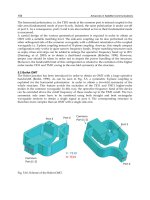
The method requires two tool transformations to be learned on the robot arm (Fig. 10(b)). The
first one, T
L
, sets the robot tool center point in the middle of the field of view of the laser
sensor, and also aligns the coordinate systems between the sensor and the robot arm.
Using this transform, any homogeneous 3D point P
sensor
= (X, Y, Z, 1) detected by the laser
sensor can be expressed in the robot reference frame (World) using:
P
world
= T
D K
robot
T
L
P
sensor
(2)
where T

D K
robot
represents the position of the robot arm at the moment of data acquisition from
the sensor. The robot position is computed using direct kinematics.
The second transformation, T
T
, moves the tool center point on the tip of the physical tool.
These two transformations, combined, allow the system to learn a trajectory using the 3D
vision sensor, having T
L
active, and then following the same trajectory with the physical in-
strument by switching the tool transformation to T
T
.
The learning procedure has two stages:
• Learning the coarse, low resolution trajectory (manually or automatically)
• Refining the accuracy by computing a fine, high resolution trajectory (automatically)
The coarse learning step can be either interactive or automatic. In the interactive mode, the
user positions the sensor by manually jogging the robot until the edge to be tracked arrives in
the field of view of the sensor, as in Fig. 10(a). The edge is located automatically in the laser
plane by a 2D vision component. In the automatic mode, the user only teaches the edge model,
the starting point and the scanning direction, and the system will advance automatically the
sensor in fixed increments, acquiring new points. For non-straight contours, the curvature is
automatically detected by estimating the tangent (first derivative) at each point on the edge.
The main advantage of the automatic mode is that it can run with very little user interaction,
while the manual mode provides more flexibility and is advantageous when the task is more
difficult and the user wants to have full control over the learning procedure.
A related contour following method, which also uses a laser-based optical sensor, is described
in (Pashkevich, 2009). Here, the sensor is mounted on the welding torch, ahead of the welding
direction, and it is used in order to accurately track the position of the seam.

4. Conclusions
This chapter presented two applications of 3D vision in industrial robotics. The first one al-
lows 3D reconstruction of decorative objects using a laser-based profile scanner mounted on
a 6-DOF industrial robot arm, while the scanned part is placed on a rotary table. The second
application uses the same profile scanner for 3D robot guidance along a complex path, which
is learned automatically using the laser sensor and then followed using a physical tool. While
the laser sensor is an expensive device, it can obtain very good accuracies and is suitable for
precise robot guidance.
5. References
Borangiu, Th., Dogar, Anamaria and A. Dumitrache (2008a), Modelling and Simulation of
Short Range 3D Triangulation-Based Laser Scanning System, Proceedings of ICCCC’08,
Oradea, Romania
Borangiu, Th., Dogar, Anamaria and A. Dumitrache (2008b), Integrating a Short Range Laser
Probe with a 6-DOF Vertical Robot Arm and a Rotary Table, Proceedings of RAAD
2008, Ancona, Italy
Borangiu, Th., Dogar, Anamaria and A. Dumitrache (2009a), Calibration of Wrist-Mounted
Profile Laser Scanning Probe using a Tool Transformation Approach, Proceedings of
RAAD 2009, Brasov, Romania
Borangiu, Th., Dogar, Anamaria and A. Dumitrache, (2009b) Flexible 3D Trajectory Teaching
and Following for Various Robotic Applications, Proceedings of SYROCO 2009, Gifu,
Japan
Calin, G. & Roda, V.O. (2007) Real-time disparity map extraction in a dual head stereo vision
system, Latin American Applied Research, v.37 n.1, Jan-Mar 2007, ISSN 0327-0793
Cheng, F. & Chen, X. (2008). Integration of 3D Stereo Vision Measurements in Industrial Robot
Applications, International Conference on Engineering & Technology, November 17-19,
2008 – Music City Sheraton, Nashville, TN, USA, ISBN 978-1-60643-379-9, Paper 34
Cignoni, P. et. al., MeshLab: an Open-Source Mesh Processing Tool Sixth Eurographics Italian
Chapter Conference, pp. 129-136, 2008.
Hardin, W. (2008). 3D Vision Guided Robotics: When Scanning Just Wonâ
˘

A
´
Zt Do, Ma-
chine Vision Online. Retrieved from />public/articles/archivedetails.cfm?id=3507
Inaba, Y. & Sakakibara, S. (2009). Industrial Intelligent Robots, In: Springer Handbook of Au-
tomation, Shimon I. Nof (Ed.), pp. 349-363, ISBN: 978-3-540-78830-0, StÃijrz GmbH,
WÃijrzburg
Iversen, W. (2006). Vision-guided Robotics: In Search of the Holy Grail, Automation World.
Retrieved from />Palmisano, J. (2007). How to Build a Robot Tutorial, Society of Robots. Retrieved from http:
//www.societyofrobots.com/sensors_sharpirrange.shtml
Pashkevich, A. (2009). Welding Automation, In: Springer Handbook of Automation, Shimon I.
Nof (Ed.), pp. 1034, ISBN: 978-3-540-78830-0, StÃijrz GmbH, WÃijrzburg
Peng, T. & Gupta, S.K. (2007) Model and algorithms for point cloud construction using digital
projection patterns. ASME Journal of Computing and Information Science in Engineering,
7(4): 372-381, 2007.
Persistence of Vision Raystracer Pty. Ltd., POV-Ray Online Documentation
RobotArmswith3DVisionCapabilities 513
A second application, described in (Borangiu et al., 2009b), uses the same profile sensor for
teaching a complex 3D path which follows an edge of an workpiece, without the need to have
a CAD model of the respective part. The 3D contour is identified by its 2D profile, and the
robot is able to learn a sequence of points along the edge of the part. After teaching, the robot
is able to follow the same path using a physical tool, in order to perform various technological
operations, for example, edge deburring or sealant dispensing. For the experiment, a sharp
tool was used, and the robot had to follow the contour as precisely as possible. Using the laser
sensor, the robot was able to teach and follow the 3D path with a tracking error of less than
0.1 milimetres.
The method requires two tool transformations to be learned on the robot arm (Fig. 10(b)). The
first one, T
L
, sets the robot tool center point in the middle of the field of view of the laser

sensor, and also aligns the coordinate systems between the sensor and the robot arm.
Using this transform, any homogeneous 3D point P
sensor
= (X, Y, Z, 1) detected by the laser
sensor can be expressed in the robot reference frame (World) using:
P
world
= T
D K
robot
T
L
P
sensor
(2)
where T
D K
robot
represents the position of the robot arm at the moment of data acquisition from
the sensor. The robot position is computed using direct kinematics.
The second transformation, T
T
, moves the tool center point on the tip of the physical tool.
These two transformations, combined, allow the system to learn a trajectory using the 3D
vision sensor, having T
L
active, and then following the same trajectory with the physical in-
strument by switching the tool transformation to T
T
.

The learning procedure has two stages:
• Learning the coarse, low resolution trajectory (manually or automatically)
• Refining the accuracy by computing a fine, high resolution trajectory (automatically)
The coarse learning step can be either interactive or automatic. In the interactive mode, the
user positions the sensor by manually jogging the robot until the edge to be tracked arrives in
the field of view of the sensor, as in Fig. 10(a). The edge is located automatically in the laser
plane by a 2D vision component. In the automatic mode, the user only teaches the edge model,
the starting point and the scanning direction, and the system will advance automatically the
sensor in fixed increments, acquiring new points. For non-straight contours, the curvature is
automatically detected by estimating the tangent (first derivative) at each point on the edge.
The main advantage of the automatic mode is that it can run with very little user interaction,
while the manual mode provides more flexibility and is advantageous when the task is more
difficult and the user wants to have full control over the learning procedure.
A related contour following method, which also uses a laser-based optical sensor, is described
in (Pashkevich, 2009). Here, the sensor is mounted on the welding torch, ahead of the welding
direction, and it is used in order to accurately track the position of the seam.
4. Conclusions
This chapter presented two applications of 3D vision in industrial robotics. The first one al-
lows 3D reconstruction of decorative objects using a laser-based profile scanner mounted on
a 6-DOF industrial robot arm, while the scanned part is placed on a rotary table. The second
application uses the same profile scanner for 3D robot guidance along a complex path, which
is learned automatically using the laser sensor and then followed using a physical tool. While
the laser sensor is an expensive device, it can obtain very good accuracies and is suitable for
precise robot guidance.
5. References
Borangiu, Th., Dogar, Anamaria and A. Dumitrache (2008a), Modelling and Simulation of
Short Range 3D Triangulation-Based Laser Scanning System, Proceedings of ICCCC’08,
Oradea, Romania
Borangiu, Th., Dogar, Anamaria and A. Dumitrache (2008b), Integrating a Short Range Laser
Probe with a 6-DOF Vertical Robot Arm and a Rotary Table, Proceedings of RAAD

2008, Ancona, Italy
Borangiu, Th., Dogar, Anamaria and A. Dumitrache (2009a), Calibration of Wrist-Mounted
Profile Laser Scanning Probe using a Tool Transformation Approach, Proceedings of
RAAD 2009, Brasov, Romania
Borangiu, Th., Dogar, Anamaria and A. Dumitrache, (2009b) Flexible 3D Trajectory Teaching
and Following for Various Robotic Applications, Proceedings of SYROCO 2009, Gifu,
Japan
Calin, G. & Roda, V.O. (2007) Real-time disparity map extraction in a dual head stereo vision
system, Latin American Applied Research, v.37 n.1, Jan-Mar 2007, ISSN 0327-0793
Cheng, F. & Chen, X. (2008). Integration of 3D Stereo Vision Measurements in Industrial Robot
Applications, International Conference on Engineering & Technology, November 17-19,
2008 – Music City Sheraton, Nashville, TN, USA, ISBN 978-1-60643-379-9, Paper 34
Cignoni, P. et. al., MeshLab: an Open-Source Mesh Processing Tool Sixth Eurographics Italian
Chapter Conference, pp. 129-136, 2008.
Hardin, W. (2008). 3D Vision Guided Robotics: When Scanning Just Wonâ
˘
A
´
Zt Do, Ma-
chine Vision Online. Retrieved from />public/articles/archivedetails.cfm?id=3507
Inaba, Y. & Sakakibara, S. (2009). Industrial Intelligent Robots, In: Springer Handbook of Au-
tomation, Shimon I. Nof (Ed.), pp. 349-363, ISBN: 978-3-540-78830-0, StÃijrz GmbH,
WÃijrzburg
Iversen, W. (2006). Vision-guided Robotics: In Search of the Holy Grail, Automation World.
Retrieved from />Palmisano, J. (2007). How to Build a Robot Tutorial, Society of Robots. Retrieved from http:
//www.societyofrobots.com/sensors_sharpirrange.shtml
Pashkevich, A. (2009). Welding Automation, In: Springer Handbook of Automation, Shimon I.
Nof (Ed.), pp. 1034, ISBN: 978-3-540-78830-0, StÃijrz GmbH, WÃijrzburg
Peng, T. & Gupta, S.K. (2007) Model and algorithms for point cloud construction using digital
projection patterns. ASME Journal of Computing and Information Science in Engineering,

7(4): 372-381, 2007.
Persistence of Vision Raystracer Pty. Ltd., POV-Ray Online Documentation
AdvancesinRobotManipulators514
Scharstein, D. & Szeliski, R. (2002). A taxonomy and evaluation of dense two-frame stereo
correspondence algorithms. International Journal of Computer Vision, 47(1/2/3):7-42,
April-June 2002.
Spong, M. W., Hutchinson, S., Vidyasagar, M. (2005). Robot Modeling and Control, John Wiley
and Sons, Inc., pp. 71-83, 2005
Robotassisted3Dshapeacquisitionbyopticalsystems 515
Robotassisted3Dshapeacquisitionbyopticalsystems
CesareRossi,VincenzoNiola,SergioSavinoandSalvatoreStrano
x

Robot assisted 3D shape
acquisition by optical systems

Cesare Rossi, Vincenzo Niola, Sergio Savino and Salvatore Strano
University of Naples “Federico II”
ITALY

1. Introduction

In this chapter, a short description of the basic concepts about optical methods for the
acquisition of three-dimensional shapes is first presented. Then two applications of the
surface reconstruction are presented: the passive technique Shape from Silhouettes and the
active technique Laser Triangolation. With both these techniques the sensors (telecameras
and laser beam) were moved and oriented by means of a robot arm. In fact, for complex
objects, it is important that the measuring device can move along arbitrary paths and make
its measurements from suitable directions. This chapter shows how a standard industrial
robot with a laser profile scanner can be used to achieve the desired d-o-f.

Finally some experimental results of shape acquisition by means of the Laser Triangolation
technique are reported.

2. Methods for the acquisition of three-dimensional shapes

In this paragraph the computational techniques are described to estimate the geometric
property (the structure) of the three-dimensional world (3D),
starting from ist
bidimensional projections (2D): the images. The shape acquisition problem ( shape/model
acquisition, image-based modeling, 3D photography) is introduced and all steps that are
necessary to obtain true tridimensional models of the objects, are synthetized [1].
Many methods for the automatic acquisition of the shape object exist. One possible
classification of the methods for shape acquisition is illustrated
in gure 1.
In this chapter optical methods will be analyze. The principal advantages of this kind of
techniques are the absence of contact, the rapidity and the economization. The limitations
include the possibility of being able to acquire only the visible part of the surfaces and the
sensibility to the property of the surfaces like transparency, brilliance and color.
The problem of image-based modeling or 3D photography, can be described in this way: the
objects irradiate visible light; the camera capture this “light“, whose characteristics depend
on the lighting system of the scene, surface geometry, reflecting surface; the computer
elaborates the light by means of opportune algorithms
to reconstruct the 3D structure of
the objects.

26
AdvancesinRobotManipulators516


Fig. 1. Classification of the methods for shape acquisition [1]

In the figure 2 is shown an equipment for the shape acquisition by means two images.


Fig. 2. Stereo acquisition

The fundamental distinction between the optical techniques for shape acquisition,
regards
the use of special lighting sources. In particular, it is possible to distinguish two kinds of
optical methods: active methods, that modify the images of scene by means of opportune
luminous pattern, laser lights, infrared radiations,
etc., and passive methods, that analyze
the images of the scene without to modify it. The active methods have the advantage to
concur high resolutions, but they are more expensive and not always applicable. The
passive methods are economic, they have fewer constraints obligatory, but they are
characterized by lower resolutions.
Many of the optical methods for the shape acquisition have like result
an image range, that
is an image in which every pixel contains the distance from the sensor, of a visible point of
the scene, instead of its brightness
(gure 3). An image range is constituted by measures

(discrete) of a 3D surface respect to a 2D plan (usual the plane image sensor) and therefore
it is also called: 2.5D image. The surface can be always expressed in the form Z = f(X, Y), if
the reference plane is XY. A sensor range
is a device that produces an image range.


Fig. 3. Brightness reconstruction of an image [1]

Below optical sensor range is any optical system of shape acquisition, active or passive, that
is composed of equipment and softwares and that gives back an image range of the scene.
The main characteristics of a sensor range are:
 resolution: the smallest change of depth that the sensor can find;
 accuracy: diffrence between measured value
(average of repeated measures) and
true value (it measures the systematic error);
 precision: statistic variation (standard deviation) of repeated measures of a same
quantity (dispersion of the measures around the average);
 velocity: number of measures in a second.

2.2 From the measure to the 3D model
The recovery of 3D information, however, does not exhaust the process of shape acquisition,
even if it is the fundamental step. In order to obtain a complete model of an object, or of a
scene, many images range are necessary, and they che they must be aligned and merged
with each other to obtain a 3D surface (like poligonal mesh).
The reconstruction of the model of the object starting from images range, previews three
steps:
 adjustment: (or alignment) in order to transform the measures supplied from the
several images range in a one common reference system;
 geometric fusion: in order to obtain a single 3D surface (typically a poligonal
mesh) starting various image range;
 mesh simplification: the points given back by a sensor range are too many to have
a manageable model and the mesh must be simplified.

Below the first phase will be described above all, the second will be summarily and the third
will be omitted.
An image range Z(X,Y) defines a set of 3D points
(X,Y,Z(X,Y)), gure 4a. In order to obtain
a surface in the 3D space (surface range) it is sufficient connect between their nearest points

with triangular surfaces (gure 4b).
Robotassisted3Dshapeacquisitionbyopticalsystems 517


Fig. 1. Classification of the methods for shape acquisition [1]

In the figure 2 is shown an equipment for the shape acquisition by means two images.


Fig. 2. Stereo acquisition

The fundamental distinction between the optical techniques for shape acquisition,
regards
the use of special lighting sources. In particular, it is possible to distinguish two kinds of
optical methods: active methods, that modify the images of scene by means of opportune
luminous pattern, laser lights, infrared radiations,
etc., and passive methods, that analyze
the images of the scene without to modify it. The active methods have the advantage to
concur high resolutions, but they are more expensive and not always applicable. The
passive methods are economic, they have fewer constraints obligatory, but they are
characterized by lower resolutions.
Many of the optical methods for the shape acquisition have like result
an image range, that
is an image in which every pixel contains the distance from the sensor, of a visible point of
the scene, instead of its brightness
(gure 3). An image range is constituted by measures

(discrete) of a 3D surface respect to a 2D plan (usual the plane image sensor) and therefore
it is also called: 2.5D image. The surface can be always expressed in the form Z = f(X, Y), if
the reference plane is XY. A sensor range

is a device that produces an image range.


Fig. 3. Brightness reconstruction of an image [1]

Below optical sensor range is any optical system of shape acquisition, active or passive, that
is composed of equipment and softwares and that gives back an image range of the scene.
The main characteristics of a sensor range are:
 resolution: the smallest change of depth that the sensor can find;
 accuracy: diffrence between measured value
(average of repeated measures) and
true value (it measures the systematic error);
 precision: statistic variation (standard deviation) of repeated measures of a same
quantity (dispersion of the measures around the average);
 velocity: number of measures in a second.

2.2 From the measure to the 3D model
The recovery of 3D information, however, does not exhaust the process of shape acquisition,
even if it is the fundamental step. In order to obtain a complete model of an object, or of a
scene, many images range are necessary, and they che they must be aligned and merged
with each other to obtain a 3D surface (like poligonal mesh).
The reconstruction of the model of the object starting from images range, previews three
steps:
 adjustment: (or alignment) in order to transform the measures supplied from the
several images range in a one common reference system;
 geometric fusion: in order to obtain a single 3D surface (typically a poligonal
mesh) starting various image range;
 mesh simplification: the points given back by a sensor range are too many to have
a manageable model and the mesh must be simplified.

Below the first phase will be described above all, the second will be summarily and the third
will be omitted.
An image range Z(X,Y) defines a set of 3D points
(X,Y,Z(X,Y)), gure 4a. In order to obtain
a surface in the 3D space (surface range) it is sufficient connect between their nearest points
with triangular surfaces (gure 4b).
AdvancesinRobotManipulators518


a) b)


Fig. 4. Image range result (a) and its surface range (b) [1].

In many cases depth discontinuities can not be covered with triangles in order to avoid
making assumptions that are unjustified on the shape of the surface. For this reason it is
desirable to eliminate triangles with sides too long and those with excessively acute angles.

2.3 Adjustment
The sensors range don’t capture the shape of an object with a single image, many images are
needed, each of which captures a part of the object surface. The portions of the surface of the
object are obtained by different images range, and each of them is made in its own reference
system ( that depends on sensor position).
The aim of adjustment is to expres all images in the same reference system, by means of an
opportune rigid transformation
(rotation and translation).
If the position and orientation of the sensor are known, the problem is resolved banally.
However in many cases, the sensor position in the space is unknown and the
transformations can be calculated using only images data, by means of opportune
algorithms, one of these is ICP (Iterated Closest Point).

In the figure
5, on the left, eight images range of an object are shown, each in its own
reference system; on the right, all images are were superimposed with adjustment
operation.


Fig. 5. Images range and result of adjustment operation [1]


2.4 Geometric fusion
After all images range data are adjusted in one reference system, they be united in a single
shape, represented, as an example, by triangular mesh. This problem of surface
reconstruction, can be formulated like an estimation of the bidimensional variety which
approximates the surface of the unknown object by starting to a set of 3D points. The
methods of geometric fusion can be divided in two
categories:

 Integration of meshes: the triangular meshes
of the single surfaces range, are
joined.
 Volumetric fusion: all data are joined in a volumetric representation, from which a
triangular mesh is extracted.

2.4.1 Integration of meshes
The techniques of integration of meshes
aim to merge several 3D overlapped triangular
meshes into a single triangular mesh (using the representation in terms of surface range).
The method of Turk and Levoy
(1994) merges overlapped triangular meshes by means of a
technique named “zippering“. The overlapping meshes are eroded to eliminate the overlap

and then it is possible to use a 2D triangolation to sew up the edges. To make this the
points of the two 3D surface close
to edges, must be projected onto a plane 2D.
In the figure
6, on the left, two aligned surface are shown, and on the right, the zippering
result is shown.


Fig. 6. Aligned surface and zippering result

The techniques of integration of meshes
allow the fusion of several images range without
losing accuracy, since the vertices of the final mesh coincide with the points of the measured
data
. But, for the same reason, the results of these techniques are sensitive to erroneous
measurements, that may cause problems in the surface reconstruction.

2.4.2 Volumetric Fusion
The volumetric fusion
of surface measurements constructs an intermediate implicit surface
that combines the measurements overlaid in a single representation. The implicit
Robotassisted3Dshapeacquisitionbyopticalsystems 519


a) b)


Fig. 4. Image range result (a) and its surface range (b) [1].

In many cases depth discontinuities can not be covered with triangles in order to avoid

making assumptions that are unjustified on the shape of the surface. For this reason it is
desirable to eliminate triangles with sides too long and those with excessively acute angles.

2.3 Adjustment
The sensors range don’t capture the shape of an object with a single image, many images are
needed, each of which captures a part of the object surface. The portions of the surface of the
object are obtained by different images range, and each of them is made in its own reference
system ( that depends on sensor position).
The aim of adjustment is to expres all images in the same reference system, by means of an
opportune rigid transformation
(rotation and translation).
If the position and orientation of the sensor are known, the problem is resolved banally.
However in many cases, the sensor position in the space is unknown and the
transformations can be calculated using only images data, by means of opportune
algorithms, one of these is ICP (Iterated Closest Point).
In the figure
5, on the left, eight images range of an object are shown, each in its own
reference system; on the right, all images are were superimposed with adjustment
operation.


Fig. 5. Images range and result of adjustment operation [1]


2.4 Geometric fusion
After all images range data are adjusted in one reference system, they be united in a single
shape, represented, as an example, by triangular mesh. This problem of surface
reconstruction, can be formulated like an estimation of the bidimensional variety which
approximates the surface of the unknown object by starting to a set of 3D points. The
methods of geometric fusion can be divided in two

categories:

 Integration of meshes: the triangular meshes
of the single surfaces range, are
joined.
 Volumetric fusion: all data are joined in a volumetric representation, from which a
triangular mesh is extracted.

2.4.1 Integration of meshes
The techniques of integration of meshes
aim to merge several 3D overlapped triangular
meshes into a single triangular mesh (using the representation in terms of surface range).
The method of Turk and Levoy
(1994) merges overlapped triangular meshes by means of a
technique named “zippering“. The overlapping meshes are eroded to eliminate the overlap
and then it is possible to use a 2D triangolation to sew up the edges. To make this the
points of the two 3D surface close
to edges, must be projected onto a plane 2D.
In the figure
6, on the left, two aligned surface are shown, and on the right, the zippering
result is shown.


Fig. 6. Aligned surface and zippering result

The techniques of integration of meshes
allow the fusion of several images range without
losing accuracy, since the vertices of the final mesh coincide with the points of the measured
data
. But, for the same reason, the results of these techniques are sensitive to erroneous

measurements, that may cause problems in the surface reconstruction.

2.4.2 Volumetric Fusion
The volumetric fusion
of surface measurements constructs an intermediate implicit surface
that combines the measurements overlaid in a single representation. The implicit
AdvancesinRobotManipulators520

representation of the surface is an iso-surface of a scalar field f(x,y,z). As an example, if the
function of field is defined as the distance of the nearest point on the surface of the object,
then the implicit surface is represented by f(x,y,z) = 0. This representation allows modeling
of the shape of unknown objects with arbitrary topology and geometry.
To switch from implicit representation of the surface to a triangular mesh, it is possible to
use the algorithm Marching Cubes, developed by
Lorensen e Cline (1987) for the
triangulation of iso-surfaces from the discrete representation of a scalar field (as the 3D
images in the medical field). The same algorithm is useful for obtaining a triangulated
surface from volumetric reconstructions of the scene (shape from silhouette and photo
consistency).
The method of Hoppe and others
(1992) neglects the structure of the data (surface range)
and calculates a surface from the unstructured "cloud" of points.
Curless and Levoy (1996) instead, take advantage of the information contained in the images
range in order to assign the voxel that lie along the sight line
that, starting from a point of
the surface range, arrives to the sensor.
An obvious limitation of all geometric fusion algorithms based on an intermediate structure
of discrete volumetric data is a reduction of accuracy, resulting in the loss of details of the
surface. Moreover the space required for the volumetric representation grows quickly when
resolution

grows.

2.5 Optical methods for the shapes acquisition
All computational techniques use some indications in order to calculate the shape of the
objects starting from the images. Below the main methods divided between active and
passive, are listed.

Passive optical methods:
 depth from focus/defocus
 shape from texture
 shape from shading
 stereo-photometric
 stereopsis
 shape from silhouette
 shape from photo-consistency
 structure from motion

Active optical methods:
 active defocus
 active stereo
 active triangolation
 interferometry
 flight time

All the active methods,
except the last one, employ one or two cameras and a source of
special light, and fall in the wider class of the methods with structured lighting system.


3. Three-dimensional reconstruction with technique: Shape from Silhouettes

In this paragraph one of the passive optical techniques of 3D reconstruction will be
introduced in detail, with some obtained results.

3.1 Principle of volumetric reconstruction from shapes
The aim of volumetric reconstruction is to create a representation that describes not only the
surface of a region, but also the space that it encloses. The hypothesis is that there is a
known and limited volume, in which the objects of interest lie. A 3D box is modelled to be
an initial volume model that contains the object. This box is divided in discrete elements
called voxels, that are three-dimensional equivalent of bidimensional pixel. The
reconstruction coincides with the assignment of a label of occupation (or color) to each
element of volume. The label of occupation is usually binary
(transparent or opaque).
Volumetric reconstruction offers some advantages compared to traditional stereopsi
techniques: it avoids the difficult problem of finding correspondences, it allows the explicit
handling of occlusions and it allows to obtain directly a three-dimensional model of the
object (it is not necessary to align parts of the model) integrating simultaneously all sights

(which are the order of magnitude of ten).
Like in the stereopsi, the cameras are calibrated.
Below one of the many algorithms developed for the volumetric reconstruction from
silhouettes of an object of interest is described: shape from silhouettes .
Shape From Silhouettes is well-known technique for estimating 3D shape from its multiple
2D images.
Intuitively the silhouette is the profile of an object, comprehensive of its inside part. In the
“Shape from Silhouette” technique silhouette is defined like a binary image, which value in
a certain point (x, y) underlines if the optical ray that passes for the pixel (x, y) intersects or
not the object surface in the scene. In this way, Every point of the silhouette, respectively of
value “1” or “0”, identifies an optical ray that intersects or not the object.
To store the labels of the voxel it is possible to use the octree data structure.The octree are

trees with eight ways in which each node represents a part of space and the children nodes
represents the eight divisions of that part of space (octants).

3.1.1 Szeliski algorithm
The Szeliski algorithm allows to build the volumetric model by means of octree structure.
The octree structure is constructed subdividing each cube in eight part
(octants), starting
from the root
node that represents the initial volume. Each cube has associated a color:
 black: it represents a occupied volume;
 white: it represents an empty volume;
 gray: it represents an inner node whose classification is still uncertain.
For each octant, it is necessary to verify if its projection in image i, is entire contained in the
black region. If that happens for all N shapes, the octant is labeled as
black. If instead, the
octant projection is entire contained in the background (white), also for a single camera, the
octant is labeled as
white. If one of these two cases happens, the octant becomes a leaf of the
octree and it is not more tried, otherwise, it is labeled as gray and it is subdivided in eight
parts. In order to limit the dimension of the tree, gray octants with minimal dimension, are
Robotassisted3Dshapeacquisitionbyopticalsystems 521

representation of the surface is an iso-surface of a scalar field f(x,y,z). As an example, if the
function of field is defined as the distance of the nearest point on the surface of the object,
then the implicit surface is represented by f(x,y,z) = 0. This representation allows modeling
of the shape of unknown objects with arbitrary topology and geometry.
To switch from implicit representation of the surface to a triangular mesh, it is possible to
use the algorithm Marching Cubes, developed by
Lorensen e Cline (1987) for the
triangulation of iso-surfaces from the discrete representation of a scalar field (as the 3D

images in the medical field). The same algorithm is useful for obtaining a triangulated
surface from volumetric reconstructions of the scene (shape from silhouette and photo
consistency).
The method of Hoppe and others
(1992) neglects the structure of the data (surface range)
and calculates a surface from the unstructured "cloud" of points.
Curless and Levoy (1996) instead, take advantage of the information contained in the images
range in order to assign the voxel that lie along the sight line
that, starting from a point of
the surface range, arrives to the sensor.
An obvious limitation of all geometric fusion algorithms based on an intermediate structure
of discrete volumetric data is a reduction of accuracy, resulting in the loss of details of the
surface. Moreover the space required for the volumetric representation grows quickly when
resolution
grows.

2.5 Optical methods for the shapes acquisition
All computational techniques use some indications in order to calculate the shape of the
objects starting from the images. Below the main methods divided between active and
passive, are listed.

Passive optical methods:
 depth from focus/defocus
 shape from texture
 shape from shading
 stereo-photometric
 stereopsis
 shape from silhouette
 shape from photo-consistency
 structure from motion

Active optical methods:
 active defocus
 active stereo
 active triangolation
 interferometry
 flight time

All the active methods,
except the last one, employ one or two cameras and a source of
special light, and fall in the wider class of the methods with structured lighting system.


3. Three-dimensional reconstruction with technique: Shape from Silhouettes

In this paragraph one of the passive optical techniques of 3D reconstruction will be
introduced in detail, with some obtained results.

3.1 Principle of volumetric reconstruction from shapes
The aim of volumetric reconstruction is to create a representation that describes not only the
surface of a region, but also the space that it encloses. The hypothesis is that there is a
known and limited volume, in which the objects of interest lie. A 3D box is modelled to be
an initial volume model that contains the object. This box is divided in discrete elements
called voxels, that are three-dimensional equivalent of bidimensional pixel. The
reconstruction coincides with the assignment of a label of occupation (or color) to each
element of volume. The label of occupation is usually binary
(transparent or opaque).
Volumetric reconstruction offers some advantages compared to traditional stereopsi
techniques: it avoids the difficult problem of finding correspondences, it allows the explicit
handling of occlusions and it allows to obtain directly a three-dimensional model of the

object (it is not necessary to align parts of the model) integrating simultaneously all sights

(which are the order of magnitude of ten).
Like in the stereopsi, the cameras are calibrated.
Below one of the many algorithms developed for the volumetric reconstruction from
silhouettes of an object of interest is described: shape from silhouettes .
Shape From Silhouettes is well-known technique for estimating 3D shape from its multiple
2D images.
Intuitively the silhouette is the profile of an object, comprehensive of its inside part. In the
“Shape from Silhouette” technique silhouette is defined like a binary image, which value in
a certain point (x, y) underlines if the optical ray that passes for the pixel (x, y) intersects or
not the object surface in the scene. In this way, Every point of the silhouette, respectively of
value “1” or “0”, identifies an optical ray that intersects or not the object.
To store the labels of the voxel it is possible to use the octree data structure.The octree are
trees with eight ways in which each node represents a part of space and the children nodes
represents the eight divisions of that part of space (octants).

3.1.1 Szeliski algorithm
The Szeliski algorithm allows to build the volumetric model by means of octree structure.
The octree structure is constructed subdividing each cube in eight part
(octants), starting
from the root
node that represents the initial volume. Each cube has associated a color:
 black: it represents a occupied volume;
 white: it represents an empty volume;
 gray: it represents an inner node whose classification is still uncertain.
For each octant, it is necessary to verify if its projection in image i, is entire contained in the
black region. If that happens for all N shapes, the octant is labeled as
black. If instead, the
octant projection is entire contained in the background (white), also for a single camera, the

octant is labeled as
white. If one of these two cases happens, the octant becomes a leaf of the
octree and it is not more tried, otherwise, it is labeled as gray and it is subdivided in eight
parts. In order to limit the dimension of the tree, gray octants with minimal dimension, are
AdvancesinRobotManipulators522

labeled as black. At the end of process it is possible to obtain an octree that represents 3D
object structure.
An example
of volumetric model construction with Szeliski algorithm is shown in figure 7.


Fig. 7. Model reconstruction with Szeliski algorithm

3.1.2 Proposed method
The analysis method is to define a voxel box that contains the object in three dimensional
space and to discard subsequently
those points of the initial volume that have an empty
intersection
with at least one of the cones of the shapes obtained from the acquired images.
The voxel will have only binary values, black or white.
The algorithm is performed by projecting the center of each voxel into each image plane, by
means of the known intrinsic and extrinsic camera parameters. If the projected point is not
contained in the silhouette region, the voxel is removed from the object volume model.

3.2 Images elaboration
Starting from an RGB image (figure 8), it is analized and, by means of segmentation
procedure, it is possible to obtain object silhouette reconstruction.

Fig. 8. RGB image

Segmentation is the process by means of which the image is subdivided in characteristics of
interest. This operation is based on strong intensity discontinuities or regions that introduce
homogenous intensity on the base of established criteria.
There are four kinds of
discontinuities: points, lines, edge,
or, in a generalized manner, interest points.

In order to separate an object from the image background, the method of the threshold s is
used: each point (u,v) with f(u,v) > s (f(u,v) < s) is identified like object, otherwise like
background. The described elaboration is used to identify and characterize the various
regions that are present in each image; in particular, by means of this technique it is possible
to separate the objects from the background.
The first step
is to transform RGB image in gray scale image (figure 9), in thi way the
intensity value becomes a threshold to identify the object in the image.


Fig. 9. Gray scale image

The gray scale image is a matrix, whose dimensions correspond to number of pixel along the
two directions of the sensor, and whose elements have values in range [0,255].
Subsequently, a limited set of pixel that contains the projection of the object in the image
plane, is selected, so it is possible to facilitate the segmentation procedure (figure 10).


Fig. 10. Object identification

In gray scale image, pixel with intensity f(u,v) different from that of points that are not

representative of object (background T), are chosen. This tecnique is very effective, if in the
image there is a real difference between object and background.
For each pixel (u, v) unit value or zero, respectively, is assigned, if it is an optical beam
passing through the object or not (figure 11).

Robotassisted3Dshapeacquisitionbyopticalsystems 523

labeled as black. At the end of process it is possible to obtain an octree that represents 3D
object structure.
An example
of volumetric model construction with Szeliski algorithm is shown in figure 7.


Fig. 7. Model reconstruction with Szeliski algorithm

3.1.2 Proposed method
The analysis method is to define a voxel box that contains the object in three dimensional
space and to discard subsequently
those points of the initial volume that have an empty
intersection
with at least one of the cones of the shapes obtained from the acquired images.
The voxel will have only binary values, black or white.
The algorithm is performed by projecting the center of each voxel into each image plane, by
means of the known intrinsic and extrinsic camera parameters. If the projected point is not
contained in the silhouette region, the voxel is removed from the object volume model.

3.2 Images elaboration
Starting from an RGB image (figure 8), it is analized and, by means of segmentation
procedure, it is possible to obtain object silhouette reconstruction.

Fig. 8. RGB image

Segmentation is the process by means of which the image is subdivided in characteristics of
interest. This operation is based on strong intensity discontinuities or regions that introduce
homogenous intensity on the base of established criteria.
There are four kinds of
discontinuities: points, lines, edge,
or, in a generalized manner, interest points.

In order to separate an object from the image background, the method of the threshold s is
used: each point (u,v) with f(u,v) > s (f(u,v) < s) is identified like object, otherwise like
background. The described elaboration is used to identify and characterize the various
regions that are present in each image; in particular, by means of this technique it is possible
to separate the objects from the background.
The first step
is to transform RGB image in gray scale image (figure 9), in thi way the
intensity value becomes a threshold to identify the object in the image.


Fig. 9. Gray scale image

The gray scale image is a matrix, whose dimensions correspond to number of pixel along the
two directions of the sensor, and whose elements have values in range [0,255].

Subsequently, a limited set of pixel that contains the projection of the object in the image
plane, is selected, so it is possible to facilitate the segmentation procedure (figure 10).


Fig. 10. Object identification

In gray scale image, pixel with intensity f(u,v) different from that of points that are not
representative of object (background T), are chosen. This tecnique is very effective, if in the
image there is a real difference between object and background.
For each pixel (u, v) unit value or zero, respectively, is assigned, if it is an optical beam
passing through the object or not (figure 11).

AdvancesinRobotManipulators524


Fig. 11. The computed object silhouette region

3.3 Camera calibration
It is necessary to identify all model parameters in order to obtain a good 3-D reconstruction.
Calibration is a basic procedure for the data analysis.
There are many kind of procedure to calibrate a camera system, but in this paragraph the
study of the calibration procedures will not be discussed in detail.
The aim of calibration procedure is to obtain all intrinsic and estrinsic parameters of the
camera system. Calibration procedure is based on a set of images, taken with a target placed
in different positions that are known in a base reference system. A least square optimization
allows to identify all parameters.

3.4 The proposed algorithm
The result of image elaboration is the object silhouette region for each image with pixel
coordinates and centroid coordinates of these region in image reference system, (Fig. 11).
By means of calibration parameters (intrinsic and estrinsic), it is possible to evaluate, for
each image, an homogeneous transformation matrix, between the image reference system of
each image and a base reference system.
The first step is to discretize a portion of work space by mean an opportune box divided in
voxels (figure 12). In this operation, it is necessary to choose the number of voxels, the

dimension of box and its position in a base reference system. The position of voxel is chosen
evaluating the intersections in base reference system, of the camera optical axis that pass
through silhouette centroids of at least, two images. Subsequently it is possible to divide the
initial volume model in a number of voxels according to the established precision, and it is
possible to evaluate the centers of voxels in base reference.


Fig. 12. Voxel discretization of workspace.


For each of the silhouettes, the projection of the centre of the voxels in the image plane can
be obtained as follows:

q, ,1jp, ,1i}w
~
{]M[}
~
{
jij

(1)

Where p is the number of silhouettes, q is the number of the voxels and
i
]M[ is the
transformation matrix between the base frame and the image frame.
The algorithm is performed by projecting the center of each voxel into each image plane, by
means of the known intrinsic and extrinsic camera parameters. If the projected point is not
contained in the silhouette region, the voxel is removed from the object volume model. This
yields the following relation:

mv1nu1q, ,1j}w
~
{]M[]
~
[
1
0
v
u
jpj
j















(2)

Where n and m are the number of pixels along the directions u and v, respectively. So a

matrix [A] having dimension [n,m] is written; the values of the elements of this matrix is one
if corresponds to a couple of coordinates (u,v) obtained by eq. (2) that belongs to the object
silhouette in the image; otherwise the value is zero:

jj
hk
vk,uh1a:]A[ 
(3)

A set of pixels having coordinates
)v,u( , belonging to the first silhouette, is defined as
follows:

11
)v,u(: (4)

The points of the image that belong to the silhouette are defined as follows:

mv1nu1
)v,u(0
)v,u(1
)v,u(I
1
1
1








(5)

By the product among the matrix defined in eq. (3) with the matrix in eq. (5), the following
set of indexes is obtained:

mv1nu11]I[]A[:j
1

(6)

Now the points (in the base frame) which indexes are integer numbers belonging to the set
j are considered. These points are used as starting points to repeat the same operations,
Robotassisted3Dshapeacquisitionbyopticalsystems 525


Fig. 11. The computed object silhouette region

3.3 Camera calibration
It is necessary to identify all model parameters in order to obtain a good 3-D reconstruction.
Calibration is a basic procedure for the data analysis.
There are many kind of procedure to calibrate a camera system, but in this paragraph the
study of the calibration procedures will not be discussed in detail.
The aim of calibration procedure is to obtain all intrinsic and estrinsic parameters of the
camera system. Calibration procedure is based on a set of images, taken with a target placed
in different positions that are known in a base reference system. A least square optimization
allows to identify all parameters.

3.4 The proposed algorithm

The result of image elaboration is the object silhouette region for each image with pixel
coordinates and centroid coordinates of these region in image reference system, (Fig. 11).
By means of calibration parameters (intrinsic and estrinsic), it is possible to evaluate, for
each image, an homogeneous transformation matrix, between the image reference system of
each image and a base reference system.
The first step is to discretize a portion of work space by mean an opportune box divided in
voxels (figure 12). In this operation, it is necessary to choose the number of voxels, the
dimension of box and its position in a base reference system. The position of voxel is chosen
evaluating the intersections in base reference system, of the camera optical axis that pass
through silhouette centroids of at least, two images. Subsequently it is possible to divide the
initial volume model in a number of voxels according to the established precision, and it is
possible to evaluate the centers of voxels in base reference.


Fig. 12. Voxel discretization of workspace.


For each of the silhouettes, the projection of the centre of the voxels in the image plane can
be obtained as follows:

q, ,1jp, ,1i}w
~
{]M[}
~
{
jij

(1)

Where p is the number of silhouettes, q is the number of the voxels and

i
]M[ is the
transformation matrix between the base frame and the image frame.
The algorithm is performed by projecting the center of each voxel into each image plane, by
means of the known intrinsic and extrinsic camera parameters. If the projected point is not
contained in the silhouette region, the voxel is removed from the object volume model. This
yields the following relation:

mv1nu1q, ,1j}w
~
{]M[]
~
[
1
0
v
u
jpj
j
















(2)

Where n and m are the number of pixels along the directions u and v, respectively. So a
matrix [A] having dimension [n,m] is written; the values of the elements of this matrix is one
if corresponds to a couple of coordinates (u,v) obtained by eq. (2) that belongs to the object
silhouette in the image; otherwise the value is zero:

jj
hk
vk,uh1a:]A[ 
(3)

A set of pixels having coordinates
)v,u( , belonging to the first silhouette, is defined as
follows:

11
)v,u(: (4)

The points of the image that belong to the silhouette are defined as follows:

mv1nu1
)v,u(0
)v,u(1
)v,u(I
1

1
1







(5)

By the product among the matrix defined in eq. (3) with the matrix in eq. (5), the following
set of indexes is obtained:

mv1nu11]I[]A[:j
1

(6)

Now the points (in the base frame) which indexes are integer numbers belonging to the set
j are considered. These points are used as starting points to repeat the same operations,
AdvancesinRobotManipulators526

described by eq. (2), for all the other images. This procedure is recursive and is called space
carving technique.


Fig. 13. Scheme of space carving technique.

3.5 Evaluation of the resoluction

The choosen number of voxels defines the resoluction of the reconstructed object.
Consider a volume which dimensions are l
x
, l
y
and l
z
and a discretization along the three
directions: Δ
x
, Δ
y
e Δ
z
, the object resolutions that can be obtained in the three directions are:

z
z
z
y
y
y
x
x
x
l
a;
l
a;
l

a






(7)

In figure 14 two examples of reconstruction with different resolution choices are shown.


Fig. 14. Examples of reconstructions with different resolutions.

It must be pointed out that the choice of the initial box (resolution) depends on the optical
sensor adopted. It is clear that an object near to the sensor will appear bigger than a far one,
hence the error achieved for the same unit of discretization is increased with the distance for
a given focal length.

f
w
a;
f
w
a
v
v
c
u
u

c


(8)

Obviously it must be checked that the choosen initial resolution is not bigger than the
resolution that the optical sensor can achieve. To this pourpose, once the object has been
reconstructed, the minimum dimension that can be recorded by the camera is computed by
eq. (8); the latter is compared with the resolution initially stated.
This techique is rater slow because it is necessary to project each voxel of the initial box in
the image plane of each of the photos. Moreover, a big number of phots is required and the
procedure can not be made in real –time. It must also be noted, however, that this procedure
can be used in a rater simple way in order to obtain a rough evaluation of the volume and of
the shape of an object.
This techinque is very suitable to be assisted by a robot arm. Infact the accuracy of the
reconstruction obtained depends on the number of images used, on the positions of each
viewpoint considered, on the camera’s calibration quality and on the complexity of the
object shape. By positioning the camera on the robot, it is possible to know, exactly, not only
the characteristics of the camera, but also the position of the camera reference frame in the
robot work space. Therefore the camera intrinsic and extrinsic parameters are known
without a vision system calibration and it's easy to make an elevated number of photos. That
is to say, it could be possible to obtain vision system calibration, robot arm mechanical
calibration and trajectories recording and planning.

4. Three-dimensional reconstruction by means of Laser Triangolation

The laser triangulation technique maily permits higher operating speed with a satisfacting
quality of reconstruction.

4.1 Principle of laser triangolation

In this paragraph is described a method for surface reconstruction, that uses of a linear laser
emitter and a webcam, and uses triangulation principle applied to a scanning belt on object
surface.
Camera observes the intersection between laser and object: laser line points in image frame,
are the intersections between image plane and optical rays that pass through the intersection
points between laser and object. By means of a transformation matrix, it is possible to
express the image frame coordinates, in pixel, in a local reference frame. In figure 15 a) is
shown a scheme of scanning system: {W} is local reference frame, {I} is image frame with
coordinates system {u,v}, and {L} is laser frame. {L2} is laser plane that contains laser knife
and scanning belt on the surface of object, and it coincides with (x,y) plane of laser frame {L}.
Starting from the coordinates in pixel (u,v), in image frame, it is possible to write the
coordinates of the scanning belt on the object surface, in camera frame by means of equation
(9). Camera frame is located in camera focal point figure 15 b).

Robotassisted3Dshapeacquisitionbyopticalsystems 527

described by eq. (2), for all the other images. This procedure is recursive and is called space
carving technique.


Fig. 13. Scheme of space carving technique.

3.5 Evaluation of the resoluction
The choosen number of voxels defines the resoluction of the reconstructed object.
Consider a volume which dimensions are l
x
, l
y
and l
z

and a discretization along the three
directions: Δ
x
, Δ
y
e Δ
z
, the object resolutions that can be obtained in the three directions are:

z
z
z
y
y
y
x
x
x
l
a;
l
a;
l
a







(7)

In figure 14 two examples of reconstruction with different resolution choices are shown.


Fig. 14. Examples of reconstructions with different resolutions.

It must be pointed out that the choice of the initial box (resolution) depends on the optical
sensor adopted. It is clear that an object near to the sensor will appear bigger than a far one,
hence the error achieved for the same unit of discretization is increased with the distance for
a given focal length.

f
w
a;
f
w
a
v
v
c
u
u
c


(8)

Obviously it must be checked that the choosen initial resolution is not bigger than the
resolution that the optical sensor can achieve. To this pourpose, once the object has been

reconstructed, the minimum dimension that can be recorded by the camera is computed by
eq. (8); the latter is compared with the resolution initially stated.
This techique is rater slow because it is necessary to project each voxel of the initial box in
the image plane of each of the photos. Moreover, a big number of phots is required and the
procedure can not be made in real –time. It must also be noted, however, that this procedure
can be used in a rater simple way in order to obtain a rough evaluation of the volume and of
the shape of an object.
This techinque is very suitable to be assisted by a robot arm. Infact the accuracy of the
reconstruction obtained depends on the number of images used, on the positions of each
viewpoint considered, on the camera’s calibration quality and on the complexity of the
object shape. By positioning the camera on the robot, it is possible to know, exactly, not only
the characteristics of the camera, but also the position of the camera reference frame in the
robot work space. Therefore the camera intrinsic and extrinsic parameters are known
without a vision system calibration and it's easy to make an elevated number of photos. That
is to say, it could be possible to obtain vision system calibration, robot arm mechanical
calibration and trajectories recording and planning.

4. Three-dimensional reconstruction by means of Laser Triangolation

The laser triangulation technique maily permits higher operating speed with a satisfacting
quality of reconstruction.

4.1 Principle of laser triangolation
In this paragraph is described a method for surface reconstruction, that uses of a linear laser
emitter and a webcam, and uses triangulation principle applied to a scanning belt on object
surface.
Camera observes the intersection between laser and object: laser line points in image frame,
are the intersections between image plane and optical rays that pass through the intersection
points between laser and object. By means of a transformation matrix, it is possible to
express the image frame coordinates, in pixel, in a local reference frame. In figure 15 a) is

shown a scheme of scanning system: {W} is local reference frame, {I} is image frame with
coordinates system {u,v}, and {L} is laser frame. {L2} is laser plane that contains laser knife
and scanning belt on the surface of object, and it coincides with (x,y) plane of laser frame {L}.
Starting from the coordinates in pixel (u,v), in image frame, it is possible to write the
coordinates of the scanning belt on the object surface, in camera frame by means of equation
(9). Camera frame is located in camera focal point figure 15 b).

AdvancesinRobotManipulators528
















































1
0
v
u
1000

f000
v00
u00
1
z
y
x
0yy
0xx
c
c
c
(9)

with:
(u
0
,v
0
): image frame coordinates of focal point projection in image plane;
(δ
x
, δ
y
): physical dimension of sensor pixel along direction u and v;
f: focal length.


a) b)
Fig. 15. Scheme of scanning system

It is possible to write the expression of the optical beam of a generic point in the image
frame, that can be identified by means of parameter t.









ftz
t)vv(y
t)uu(x
c
v0c
u0c
(10)

Laser frame {L} is rotated and translated respect to camera frame, the steps and their
sequence are:
Translation Δx
lc
along axis x
c
;
Translation Δy
lc
along axis y

c
;
Translation Δz
lc
along axis z
c
;
Rotation

lc
around axis z
c
;
Rotation

lc
around axis y
c
;
Rotation

lc
around axis x
c
;
Hence in equation (11) the transformation matrix between laser frame and camera frame is:


 







































































































1000
0100
0010
x001
1
000
0100
y010
0001
1000
z100
0010
0001
1000
0100
00)cos()sin(
00)sin()cos(
1000
0)cos(0)sin(
0010
0)sin(0)cos(
1000

0)cos()sin(0
0)sin()cos(0
0001
T
lc
lc
lc
lclc
lclc
lclc
lclc
lclc
lclc
l
c
(11)

Laser plane {L2} coincides with (x,y) plane of laser frame {L}, so it contains three points:





 
T
l
T
l
T
l

}1,1,0,0{r;}1,0,0,1{q;}1,0,0,0{p 
(12)

In camera frame:



 
 
 
 
 
l
1
l
cT
czyx
l
1
l
c
T
czyx
l
1
l
cT
czyx
rT}1,r,r,r{;qT
}1,q,q,q{;pT}1,p,p,p{





(13)

It is possible to obtain laser plane equation in camera frame, solving equation (14) in xc, yc
and zc.

0
prprpr
pqpqpq
pzpypx
det
zzyyxx
zzyyxx
zcycxc















(14)

If it is:

































yyxx
yyxx
z
zzxx
zzxx
y
zzyy
zzyy
x
prpr
pqpq
detM
;
prpr
pqpq
detM;
prpr
pqpq
detM


equation in camera frame, is:

0M)pz(M)py(M)px(

zzcyycxxc






(15)

It is possible to evaluate coordinates xc, yc e zc, in camera frame, solving system (16) with
unknown t:

Robotassisted3Dshapeacquisitionbyopticalsystems 529

















































1
0
v
u
1000
f000
v00
u00
1
z
y
x
0yy
0xx
c
c
c
(9)

with:
(u
0
,v
0
): image frame coordinates of focal point projection in image plane;
(δ
x
, δ
y
): physical dimension of sensor pixel along direction u and v;

f: focal length.


a) b)
Fig. 15. Scheme of scanning system

It is possible to write the expression of the optical beam of a generic point in the image
frame, that can be identified by means of parameter t.









ftz
t)vv(y
t)uu(x
c
v0c
u0c
(10)

Laser frame {L} is rotated and translated respect to camera frame, the steps and their
sequence are:
Translation Δx
lc
along axis x

c
;
Translation Δy
lc
along axis y
c
;
Translation Δz
lc
along axis z
c
;
Rotation

lc
around axis z
c
;
Rotation

lc
around axis y
c
;
Rotation

lc
around axis x
c
;

Hence in equation (11) the transformation matrix between laser frame and camera frame is:


 






































































































1000
0100
0010
x001
1
000
0100
y010
0001
1000
z100
0010
0001
1000
0100
00)cos()sin(
00)sin()cos(

1000
0)cos(0)sin(
0010
0)sin(0)cos(
1000
0)cos()sin(0
0)sin()cos(0
0001
T
lc
lc
lc
lclc
lclc
lclc
lclc
lclc
lclc
l
c
(11)

Laser plane {L2} coincides with (x,y) plane of laser frame {L}, so it contains three points:

   
 
T
l
T
l

T
l
}1,1,0,0{r;}1,0,0,1{q;}1,0,0,0{p 
(12)

In camera frame:



 
 
 
 
 
l
1
l
cT
czyx
l
1
l
c
T
czyx
l
1
l
cT
czyx

rT}1,r,r,r{;qT
}1,q,q,q{;pT}1,p,p,p{




(13)

It is possible to obtain laser plane equation in camera frame, solving equation (14) in xc, yc
and zc.

0
prprpr
pqpqpq
pzpypx
det
zzyyxx
zzyyxx
zcycxc















(14)

If it is:

































yyxx
yyxx
z
zzxx
zzxx
y
zzyy
zzyy
x
prpr
pqpq
detM
;
prpr
pqpq
detM;
prpr
pqpq
detM


equation in camera frame, is:

0M)pz(M)py(M)px(
zzcyycxxc
 (15)

It is possible to evaluate coordinates xc, yc e zc, in camera frame, solving system (16) with
unknown t:

AdvancesinRobotManipulators530












0M)pz(M)py(M)px(
ftz
t)vv(y
t)uu(x
zzcyycxxc
c
y0c
x0c
(16)

The solution is:

zyyoxxo
zzyyxx
fMM)vv(M)uu(
MpMpMp
t




(17)

Equation (17) permits to compute in the camera frame, the points coordinates of the
scanning belt on the object surfaces, starting to its image coordinates (u,v). In this way it is
possible to carry out a 3-D objects reconstruction by means of a laser knife.

4.2 Detection of the laser path
A very important step for 3-D reconstruction is image elaboration for the laser path on the
target, [5, 6, 7] , the latter is shown in figure 16.


Fig.16. Laser path image.

Image elaboration procedure permits to user to choose some image points of laser line, in
order to identify three principal colours (Red, Green, and Blue) of laser line, figure 17.


Fig. 17. Image matrix representation.

With mean values of scanning belt principal colours, it is possible to define a brightness
coefficient of the laser line, according to relation (18):



2
))B(mean),G(mean),R(meanmin())B(mean),G(mean),R(meanmax(
s


(18)

By means of relation (19), an intensity analysis is carried out on RGB image.

2
)B,G,Rmin()B,G,Rmax(
)v,u(L


(19)

By equation (19), the matrix that contains the three layers of RGB image, is transformed in a
matrix L, that represents image intensity. This matrix represents same initial image, but it
gives information only about luminous intensity in each image pixel, and so it is a grayscale
expression of initial RGB image, figure 18 a) and b).


a) b) c)
Fig. 18. a)RGB initial image ; b)grayscale initial image L ; c) matrix Ib.

With relation (20), it is possible to define a logical matrix Ib. Matrix Ib indicates pixels of
matrix L with a brightness in a range of 15% brightness coefficient s.






otherwise0
s15.1)v,u(Ls85.0se1
)v,u(I
b
(20)

In figure 18 c), matrix Ib is shown.


Fig. 19. I
b
representation.

In matrix Ib, the scanning belt on the object surface (see fig. 19) is represented by means of
the pixel value one. The area of the laser path in the image plane depends on the real
dimension of laser beam and on external factors such as: reflection phenomena, inclination
of object surfaces.
3-D reconstruction procedure is based on triangulation principle and it doesn’t consider the
laser beam thickness, so it is necessary to associate a line to the image of scanning belt.
Robotassisted3Dshapeacquisitionbyopticalsystems 531












0M)pz(M)py(M)px(
ftz
t)vv(y
t)uu(x
zzcyycxxc
c
y0c
x0c
(16)

The solution is:

zyyoxxo
zzyyxx
fMM)vv(M)uu(
MpMpMp
t





(17)

Equation (17) permits to compute in the camera frame, the points coordinates of the
scanning belt on the object surfaces, starting to its image coordinates (u,v). In this way it is
possible to carry out a 3-D objects reconstruction by means of a laser knife.

4.2 Detection of the laser path
A very important step for 3-D reconstruction is image elaboration for the laser path on the
target, [5, 6, 7] , the latter is shown in figure 16.


Fig.16. Laser path image.

Image elaboration procedure permits to user to choose some image points of laser line, in
order to identify three principal colours (Red, Green, and Blue) of laser line, figure 17.


Fig. 17. Image matrix representation.

With mean values of scanning belt principal colours, it is possible to define a brightness
coefficient of the laser line, according to relation (18):



2
))B(mean),G(mean),R(meanmin())B(mean),G(mean),R(meanmax(
s



(18)

By means of relation (19), an intensity analysis is carried out on RGB image.

2
)B,G,Rmin()B,G,Rmax(
)v,u(L


(19)

By equation (19), the matrix that contains the three layers of RGB image, is transformed in a
matrix L, that represents image intensity. This matrix represents same initial image, but it
gives information only about luminous intensity in each image pixel, and so it is a grayscale
expression of initial RGB image, figure 18 a) and b).


a) b) c)
Fig. 18. a)RGB initial image ; b)grayscale initial image L ; c) matrix Ib.

With relation (20), it is possible to define a logical matrix Ib. Matrix Ib indicates pixels of
matrix L with a brightness in a range of 15% brightness coefficient s.






otherwise0

s15.1)v,u(Ls85.0se1
)v,u(I
b
(20)

In figure 18 c), matrix Ib is shown.


Fig. 19. I
b
representation.

In matrix Ib, the scanning belt on the object surface (see fig. 19) is represented by means of
the pixel value one. The area of the laser path in the image plane depends on the real
dimension of laser beam and on external factors such as: reflection phenomena, inclination
of object surfaces.
3-D reconstruction procedure is based on triangulation principle and it doesn’t consider the
laser beam thickness, so it is necessary to associate a line to the image of scanning belt.
AdvancesinRobotManipulators532

Since the laser path in the image plane is rather horizontal, a geometrical mean is
computed on, on the columns of the matrix Ib , that is to say: in the opposite direction to
wider extension of the laser path in the image. This is shown in equation (21).

}0)v,u(I:vv,
)v,u(I
)v,u(uI
u{
}v,u{:};v,u{:
v,u

b
v,u
b
v,u
b










(21)

Then a matrix hp is also defined as follows:









otherwise0
}v,u{se1
)v,u(h

b
(22)

Matrix hb is hence a logical matrix with same dimension of Ib in which that represents laser
image like a line, figure 20. This line is centre line of scanning belt on object surface in
image.


Fig. 20. h
b
representation.

The set of transformations (19), (20) and (21) represents the image elaboration, that is
necessary to identify a laser line in image. The points of this line are used in 3-D
reconstruction procedure.

4.3 Calibration procedure
It is necessary to identify all model parameters in order to obtain a good 3-D reconstruction.
Calibration is a basic procedure for the data analysis, [4, 6, 8]. For this reason, it was
developed a calibration procedure for a classic laser scanner module.
The laser scanner module is composed by a web-cam with resolution 640x480 pixel and a
linear laser. The calibration test rig is realized with a guide on which is fixed the laser
scanner module and a digital micrometer with a target, figure 21 a).




a) b)
Fig. 21. a) Laser scanner module calibration test rig; b) fixed frame O
f

x
f
y
f
z
f
.

A fixed frame O
f
x
f
y
f
z
f
has origin in a vertex of the rectangular target with dimension a=68
mm and b=74.5 mm, like it is shown in figure 21 b). Target movements are indicated with
Δzbf.
In figure 22 some steps of calibration procedure are shown.


Fig. 22. Calibration procedure steps.

Calibration procedure is based on a set of images, taken with the target placed in different
positions respect to the laser scanner module. A least square optimization allows to identify
all parameters. In figure 23 are shown 10 images used for calibration, of scanning belt, with
10 different Δzb
f
.

Fig. 23. Images used for calibration.

The aim of calibration procedure is to obtain the parameters that define the relation between
laser frame LxLyLzL and camera frame O
c
x
c
y
c
z
c
, figure 15.
In every calibration step, it is possible to define transformation matrix between fixed frame
O
f
x
f
y
f
z
f
and target frame:



]1000;z100;0010;0001[T
i
fb

i
b
f

(23)

Robotassisted3Dshapeacquisitionbyopticalsystems 533

Since the laser path in the image plane is rather horizontal, a geometrical mean is
computed on, on the columns of the matrix Ib , that is to say: in the opposite direction to
wider extension of the laser path in the image. This is shown in equation (21).

}0)v,u(I:vv,
)v,u(I
)v,u(uI
u{
}v,u{:};v,u{:
v,u
b
v,u
b
v,u
b











(21)

Then a matrix hp is also defined as follows:









otherwise0
}v,u{se1
)v,u(h
b
(22)

Matrix hb is hence a logical matrix with same dimension of Ib in which that represents laser
image like a line, figure 20. This line is centre line of scanning belt on object surface in
image.


Fig. 20. h
b
representation.

The set of transformations (19), (20) and (21) represents the image elaboration, that is
necessary to identify a laser line in image. The points of this line are used in 3-D
reconstruction procedure.

4.3 Calibration procedure
It is necessary to identify all model parameters in order to obtain a good 3-D reconstruction.
Calibration is a basic procedure for the data analysis, [4, 6, 8]. For this reason, it was
developed a calibration procedure for a classic laser scanner module.
The laser scanner module is composed by a web-cam with resolution 640x480 pixel and a
linear laser. The calibration test rig is realized with a guide on which is fixed the laser
scanner module and a digital micrometer with a target, figure 21 a).




a) b)
Fig. 21. a) Laser scanner module calibration test rig; b) fixed frame O
f
x
f
y
f
z
f
.

A fixed frame O
f
x
f

y
f
z
f
has origin in a vertex of the rectangular target with dimension a=68
mm and b=74.5 mm, like it is shown in figure 21 b). Target movements are indicated with
Δzbf.
In figure 22 some steps of calibration procedure are shown.


Fig. 22. Calibration procedure steps.

Calibration procedure is based on a set of images, taken with the target placed in different
positions respect to the laser scanner module. A least square optimization allows to identify
all parameters. In figure 23 are shown 10 images used for calibration, of scanning belt, with
10 different Δzb
f
.


Fig. 23. Images used for calibration.

The aim of calibration procedure is to obtain the parameters that define the relation between
laser frame LxLyLzL and camera frame O
c
x
c
y
c
z

c
, figure 15.
In every calibration step, it is possible to define transformation matrix between fixed frame
O
f
x
f
y
f
z
f
and target frame:



]1000;z100;0010;0001[T
i
fb
i
b
f

(23)

AdvancesinRobotManipulators534

The transformation matrix between fixed frame O
f
x
f

y
f
z
f
and camera frame O
c
x
c
y
c
z
c
can be
optained analogous to matrix [
c
T
l
], and it is a function of six parameters:



)(f),,,z,y,x(fT
cfcfcfcfcfcfcf
c
f
 (24)

with πcf set of parameter of transformation [
f
T

c
].
Equation (11) can be written as:



)(f),,,z,y,x(gT
lclclclclclclcl
c
 (25)

with πlc set of parameter of transformation [
c
T
l
].
For each step of the calibration procedure it is possible to evaluate the coordinates of the
points of the laser line in the camera frame, according to equations (13) and (21):

T
i
lc
T
iccc
}1,0,v,u{)f,(f}1,z,y,x{  (26)

By means of equation (22), it is possible to write:




 
T
i
lccf
T
i
lc
1
c
f
T
iccc
1
c
fT
i
fff
}1,0,v,u{)f,,(}1,0,v,u{)f,(fT
}1,z,y,x{T}1,z,y,x{




(27)

The optimization problem can be defined as:

2
R
)(Fmin

13


(28)

F(ρ) is a vectorial function defined as:

T1
f
1
f
i
f
i
f
i
f
i
f
i
f
i
f
1i
bf
1i
bf
i
f
1i

f
)}zmin(),ymin(),ymin()ymax(
),zmin()zmax(,a)xmax(
),xmin(),zz()zz{()(F




(29)

With a least square optimization, the unknown parameters of set [πcf, πlc, f] are identified.
An interactive GUI was developed to allow the user to acquire images, to execute
optimization and to verify the results.
In figure 24, a graphical result of calibration is shown: it is possible to observe the camera
frame position, the laser beam (represented by the quadrilateral on the left), and the 3-D
reconstructions of scanning beam on target surface, for each image used in the calibration
procedure.



Fig. 24. Calibration results

4.4 System accuracy
4.4.1 Camera error
An obvious source of camera calibration error arises from the spatial quantization of the
image. However, many times the image event of interest spans many pixels. It is then
possible to calculate the centroid of this event to sub-pixel accuracy, thereby reducing the
spatial quantization error. Limiting the sub-pixel accuracy is the fact that in general the
perspective projection of an object’s centroid does not equal the centroid of the object’s
perspective projection. However, often times the error incurred from assuming the centroid

of the projection is the projection of the centroid is quite small [14].
Camera accuracy is a function of its distance from observed object.
If an unitary variation of pixels in the directions u and v is considered, from the equation
(10) is gotten:

f
z
)v1v(y
f
z
)u1u(x
c
y0c
c
x0c


(30)
Calculating the difference respectively between x
c
and y
c
after and before the variation is
gotten the accuracy of the system, that is the variation of x
c
and y
c
that it can be gotten for a
minimum variation in terms of pixels in the image frame:

)v(y)1v(yy
)u(x)1u(xx
ccc
ccc



The image accuracies in directions x
c
and y
c
are:

f
z
a
c
u
x
c


Robotassisted3Dshapeacquisitionbyopticalsystems 535

The transformation matrix between fixed frame O
f
x
f
y
f

z
f
and camera frame O
c
x
c
y
c
z
c
can be
optained analogous to matrix [
c
T
l
], and it is a function of six parameters:



)(f),,,z,y,x(fT
cfcfcfcfcfcfcf
c
f
 (24)

with πcf set of parameter of transformation [
f
T
c
].

Equation (11) can be written as:



)(f),,,z,y,x(gT
lclclclclclclcl
c
 (25)

with πlc set of parameter of transformation [
c
T
l
].
For each step of the calibration procedure it is possible to evaluate the coordinates of the
points of the laser line in the camera frame, according to equations (13) and (21):

T
i
lc
T
iccc
}1,0,v,u{)f,(f}1,z,y,x{  (26)

By means of equation (22), it is possible to write:



 
T

i
lccf
T
i
lc
1
c
f
T
iccc
1
c
fT
i
fff
}1,0,v,u{)f,,(}1,0,v,u{)f,(fT
}1,z,y,x{T}1,z,y,x{




(27)

The optimization problem can be defined as:

2
R
)(Fmin
13



(28)

F(ρ) is a vectorial function defined as:

T1
f
1
f
i
f
i
f
i
f
i
f
i
f
i
f
1i
bf
1i
bf
i
f
1i
f
)}zmin(),ymin(),ymin()ymax(

),zmin()zmax(,a)xmax(
),xmin(),zz()zz{()(F




(29)

With a least square optimization, the unknown parameters of set [πcf, πlc, f] are identified.
An interactive GUI was developed to allow the user to acquire images, to execute
optimization and to verify the results.
In figure 24, a graphical result of calibration is shown: it is possible to observe the camera
frame position, the laser beam (represented by the quadrilateral on the left), and the 3-D
reconstructions of scanning beam on target surface, for each image used in the calibration
procedure.



Fig. 24. Calibration results

4.4 System accuracy
4.4.1 Camera error
An obvious source of camera calibration error arises from the spatial quantization of the
image. However, many times the image event of interest spans many pixels. It is then
possible to calculate the centroid of this event to sub-pixel accuracy, thereby reducing the
spatial quantization error. Limiting the sub-pixel accuracy is the fact that in general the
perspective projection of an object’s centroid does not equal the centroid of the object’s
perspective projection. However, often times the error incurred from assuming the centroid
of the projection is the projection of the centroid is quite small [14].
Camera accuracy is a function of its distance from observed object.

If an unitary variation of pixels in the directions u and v is considered, from the equation
(10) is gotten:

f
z
)v1v(y
f
z
)u1u(x
c
y0c
c
x0c


(30)
Calculating the difference respectively between x
c
and y
c
after and before the variation is
gotten the accuracy of the system, that is the variation of x
c
and y
c
that it can be gotten for a
minimum variation in terms of pixels in the image frame:

)v(y)1v(yy
)u(x)1u(xx

ccc
ccc



The image accuracies in directions x
c
and y
c
are:

f
z
a
c
u
x
c
