Advances in Lasers and Electro Optics Part 14 docx

27
Fundamentals and Applications
of Quantum Limited Optical Imaging
Warwick P. Bowen
1
, Magnus T. L. Hsu
1
and Jian Wei Tay
2

1
School of Mathematics and Physics, University of Queensland, QLD 4072
2
Physics Department, University of Otago, Dunedin
1
Australia
2
New Zealand
1. Introduction
The field of optical imaging is focussed on techniques to extract useful information about a
physical system from the spatial structure of light. There are two main themes to research in
this field, the resolving of previously unknown structures ranging in size from microns in
microscopy to distant galaxies in astronomical telescopy; or if the structure is selected from
an a priori known set, then its unique discrimination, such as in data read-out from a CD or
DVD. In general, both types of imaging involve the collection and focusing of light after
interaction with the object. However, the process of information extraction can be quite
different. In resolving an unknown structure, a full two dimensional image is usually
desired. Here, the metric of success is generally the resolution of the final image. In most
cases diffraction is the key concern, presenting the diffraction limit to the resolution of the
final image as approximated by Abbe (Born & Wolf, 1999). There are ways to overcome this
limit, such as by utilising non-linearities (Hell et al., 2009), or using metamaterials (Pendry,

2000) to form so called superlenses, and this is a vibrant and growing area of research.
The focus of this Chapter, however, is on the second theme of imaging, discrimination
between a set of known structures. As we will see, this form of imaging is important, not
only for read-out of information from data storage devices, but also in other areas such as
microscopy (Fabre et al., 2000; Tay et al., 2009) and satellite navigation (Arnon, 1998; Nikulin
et al., 2001). In structure discrimination, the goal is not to achieve a two dimensional image,
but rather to generate a signal which unambiguously distinguishes each element of the set.
Hence, the diffraction limit and other constraints on imaging resolution are no longer the
primary concern, but rather the signal-to-noise ratio with which the discrimination may be
performed. To maximise the signal the optical measurement must be matched carefully to
the set of structures to be discriminated; whereas the noise typically comes from electronic,
environmental, and optical sources. Much engineering effort has been applied to minimising
the noise sources for important imaging systems; however, fundamentally the quantisation
of light imposes the quantum noise limit (QNL) which is outside of engineering control. In
this Chapter we consider a general imaging system, and show how the optical mode
carrying full signal information may be determined. We introduce spatial homodyne
detection (Beck, 2000; Hsu et al., 2004) as a method to optimally extract this signal, showing
Advances in Lasers and Electro Optics

634
how the QNL to measurement sensitivity may be determined and even surpassed using
non-classical states of light. We illustrate the implications of these techniques for two key
imaging systems, atomic force microscopy (Binning et al., 1985; Fabre et al., 2000) and
particle tracking in optical tweezers (Block, 1992; Tay et al., 2009); comparing optimal spatial
homodyne based signal extraction to the standard extraction methods used in such systems
today.
2. Quantum formalism for optical measurements
The field of optical measurements has progressed significantly, with photo-detection
techniques advancing from the use of the photographic plate in the 19th century to the
semiconductor-based photodetectors commonly encountered today. One is now able to

measure with high accuracy and speed, the range of parameters that describe an optical
field. For example, the amplitude and phase quadratures, the Stokes polarisation
parameters, and the transverse spatial profile that are commonly used to parameterise the
optical field (Walls & Milburn, 1995). These parameters can be measured and quantified
using a range of detection techniques such as interferometry, polarimetry and beam
profiling (Saleh & Teich, 1991). However, experimentally measured values for these
parameters are estimates due to the presence of classical and quantum noise, and detection
inefficiencies.


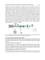
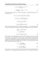
Fig. 1. Schematics of (a) a Michelson interferometer with an inset photo of the Laser
Interferometer Gravity-wave Observatory (LIGO), (b) a polarimeter with inset photo of an
on-chip polarimeter, and (c) an optical microscope with an inset photo of an optical
microscope. M: mirror, BS: beam-splitter and PBS: polarising beam-splitter.
Fig. 1 shows examples of techniques used for the measurement of (a) amplitude and phase
quadratures (Slusher et al., 1985), (b) polarization (Korolkova & Chirkin, 1996) and (c) spatial
variables (Pawley, 1995). Fig. 1 (a) shows a Michelson interferometer whereby an input field
is split using a beam-splitter, followed by propagation of the two output fields through
different paths with an effective path difference. These two fields are then interfered to
produce an output interference signal. Depending on the effective path difference,
destructive or constructive interference is obtained at the output of the interferometer.
Variations of this technique include the Mach-Zehnder (Mach, 1892; Zehnder, 1891) and
Sagnac (Sagnac, 1913) interferometers. A polarimeter is shown in Fig. 1 (b), where an input
field is phase retarded and the different polarisation components of the input field are
separated using a polarization beam-splitter. A measurement of the intensity difference
Fundamentals and Applications of Quantum Limited Optical Imaging

635
between the different polarization components provides information on the Stokes variables
that characterise the polarization phase space (Bowen et al., 2002). Interferometry and

polarimetry are essentially single spatial mode techniques, since the spatial discrimination
of the field structure cannot be characterized with these techniques. In order to reach their
measurement sensitivity limits, classical noise sources have to be reduced (or eliminated)
sufficiently such that quantum noise becomes the dominant noise source. Consequently,
optimal measurements of the amplitude and phase quadratures as well as the polarisation
variables are obtained, with measurement sensitivity bounded at the QNL.
Measurements of the spatial properties of light are more complex, since multiple spatial
modes are naturally involved. Therefore noise sources are no longer the sole consideration,
with the modal selection and filtration processes also becoming critical. Fig. 1 (c) shows a
schematic of an optical microscope, where a focused light field is used to illuminate and
image a microscopic sample. Existing techniques to resolve the finer spatial details of an
optical image include for example the filtration of different spatial frequency components
via confocal microscopy (Pawley, 1995); or the collection of non-propagating evanescent
modes that decay exponentially over wavelength-scales via near-field microscopy (Synge,
1928).
Here we are interested in the procedure of optimal parameter measurement, as shown in
Fig. 2, whereby the detection system is tailored to optimally extract a specific spatial signal.
An input field is spatially perturbed (i.e. a spatial signal is applied to the optical field, be it
known or unknown), and the resultant field is detected. To be able to optimally measure the
perturbation applied to the field, the relevant signal field components have to be identified
and resolved.



Fig. 2. The optimal parameter measurement procedure. An input field is perturbed by some
known or unknown spatial signal and the resultant field is detected. Optimal measurements
of the perturbation can be performed by identifying and resolving the relevant signal field
components.
Advances in Lasers and Electro Optics

636
We now present a formalism for defining the quantum limits to measurements of spatial
perturbations of an optical field. The spatial perturbation, quantified by parameter p is
entirely arbitrary, and could for instance be the displacement or rotation of a spatial mode in
the transverse plane (Hsu et al., 2004; 2009), or the perturbation introduced by an
environmental factor such as scattering from a particle within the field or atmospheric
fluctuations.
In general, the optical field requires a full three dimensional description using Maxwell’s
equations (Van de Hulst, 1981). In systems where all dimensions are significantly larger than
the optical wavelength, however, the paraxial approximation can usually be invoked and
the field can be described using two dimensional transverse spatial modes in a convenient
basis. The spatial quantum states of an optical field exist within an infinite dimensional
Hilbert space, and may be conveniently expanded in the basis of the rectangularly-
symmetric TEM
mn
or circularly-symmetric LG
nl
modes, with the choice of modal basis
dependent on the spatial symmetry of the imaged optical field.
A field of frequency
ω
can be represented by the positive frequency part of the electric field
operator Following Tay et al. (2009), the transverse information of the field is
described fully by the slowly varying field envelope operator
+
(
ρ
), given by

(1)

where
ρ
= (x,y) is a co-ordinate in the transverse plane of the field, V is the volume of the
optical mode, and the summation over the parameters j, m and n is given by

(2)
The respective transverse beam amplitude function and the photon annihilation operator
are given by (
ρ
) and with polarisation denoted by the superscript j. The u
mn
(
ρ
)
mode functions are normalized such that their self-overlap integrals are unity, with the
inner product given by

(3)
An arbitrary spatial perturbation, described by parameter p, is now applied to the field. Eq.
(1) can therefore be expressed as a sum of coherent amplitude components and quantum
noise operators, given by

(4)
Fundamentals and Applications of Quantum Limited Optical Imaging

637
where
being the coherent amplitude
of mode v(
ρ

, p), and

is the unit polarisation vector. From Eq. (4), one can then relate

(p)
and v(
ρ
, p) to
+
(
ρ
, p) by

(5)

(6)
where , and the normalization constant N
v
is given by

(7)
The mean number of photons passing through the transverse plane of the field per second is
given by |
(p)|
2
. We also assume, without loss of generality, that (p) is real. The quantum
noise operator carrying all of the noise on the field in mode u
mn
(
ρ

) = (
ρ
,0) is given by
δ
=

= 〈 〉.
In the limit of small estimate parameter p, we can take the first order Taylor expansion of the
first bracketed term in Eq. (4), given by

(8)
where the first term on the right-hand side of Eq. (8) indicates that the majority of the power
of the field is in the v(
ρ
,0) mode. The second term defines the spatial mode w(
ρ
)
corresponding to small changes in the parameter p, given by

(9)
where N
w
is the normalisation given by

(10)
Notice that the first term in Eq. (8) is independent of p; while the second term, and therefore
the amplitude of mode w(
ρ
), is directly proportional to p. Therefore, by measuring the
amplitude of mode w(

ρ
) it is possible to extract all available information about p. As a
consequence, we henceforth term w(
ρ
) the signal mode.
3. Detection systems
Several techniques have been developed to experimentally quantify the amplitude of the
signal mode. Here we discuss the three most common of such: array detection, split
detection, and spatial homodyne detection, as shown in Fig. 3.
Advances in Lasers and Electro Optics

638

Fig. 3. Detection systems for the measurement of the spatial properties of the field. (a) Array,
(b) split and (c) spatial homodyne detection systems. BS: beam-splitter, LO: local oscillator
field, CCD: charge-coupled detector, QD: quadrant detector (four component split detector),
SLM: spatial light modulator.
3.1 Array detection
As shown in Fig. 3 (a) array detectors in general consist of an m ×n array of pixels each of
which generates a photocurrent proportional to its incident optical field intensity. One
subclass of array detectors is the ubiquitous charge-coupled device (CCD), which is the most
common form of detector used for characterisation of the spatial properties of light beams.
To the authors knowledge, the first quantum treatment of optical field detection using array
detectors was given in Beck (2000). In this work Beck (2000) proposed the use of two array
detectors with a local oscillator in a homodyne configuration to perform spatial homodyne
detection. Such techniques will be discussed in detail in section 3.3. Quantum measurements
with a simple single array were first considered later in papers by Treps, Delaubert and
others (Treps et al., 2005; Delaubert et al., 2008). An ideal array detector consists of a two
dimensional array of infinitesimally small pixels, each with unity quantum efficiency, and
each registering the amplitude of its incident field with high bandwidth. However, realistic

array detectors stray far from this ideal; with efficiencies generally around 70 % due both to
the intrinsic inefficiency of the pixels and due to dead zones between pixels, complications
in shift register readout, and bandwidth limitations
1
. To date, all quantum imaging
experiments utilising array detectors have been performed in the context of spatial
homodyne detection. We therefore defer further discussion of these techniques to Section 3.3.
3.2 Split detection
One of the most important spatial parameters of an optical beam is the fluctuation of its
mean position, commonly termed optical beam displacement, which provides extremely
sensitive information about environmental perturbations such as forces exerted on
microscopic systems (see Sections 4 and 5), mechanical vibrations, and air turbulence; as
well as control information in techniques such as satellite navigation (Arnon, 1998; Nikulin
et al., 2001)) and locking of optical resonators (Shaddock et al., 1999), to name but a few. The
most convenient means to measure optical beam displacement is through measurement on a
split detector (Putman et al., 1992; Treps et al., 2002; 2003), as shown in Figure 3 (b). Such
detectors are composed of two or more PIN photodetectors arranged side-by-side. So long

1
For example, to achieve a typical quantum imaging detection bandwidth of 1 MHz, a 10-bit
10 megapixel CCD camera would require a total bit transfer rate of 100 T-bits/s.
Fundamentals and Applications of Quantum Limited Optical Imaging

639
as the optical field is aligned to impinge equally on the two photodetectors, and the optical
beam shape is well behaved, the difference between the output photocurrents provides a
signal proportional to the beam displacement. Furthermore, since only a pair of PIN
photodiodes is used, both the efficiency and bandwidth issues related to array detection are
easily resolved. The limitation of split detectors, however, is that they are restricted to
measurement of a certain subset of signal modes, and therefore, in general will not be

optimal for a given application (Hsu et al., 2004). Here we derive the split detection signal
mode following the treatments of Hsu et al. (2004) and Tay et al. (2009). The sensitivity
achievable in the measurement of a general signal mode will be treated later in Section 3.4.
The difference photocurrent output from a split detector can in general be written as


(11)

(12)
This can be shown (Fabre et al., 2000) to be equal to

(13)
where

is the amplitude quadrature operator of a flipped mode with mode
intensity equal to that of the incident field but a
π
phase flip about the split between
photodiodes. The transverse mode amplitude function of the flipped mode is given by

(14)
It is useful to separate the flipped mode amplitude quadrature operator into a coherent
amplitude component

(15)
which contains the signal due to the parameter p; and a quantum noise operator


which places a quantum limit on the measurement sensitivity, so that

(16)
Hence, we see that split detection measures the signal and noise in a flipped version of the
incident mode.
3.3 Spatial homodyne detection
Spatial homodyne detection was first proposed by Beck (2000) using array detectors, and
was extended to the case of pairs of PIN photodiodes with a spatially tailored local oscillator
field by Hsu et al. (2004). Spatial homodyne detection has the significant advantage over
split detection in that the detection mode can be optimised to perfectly match the signal
mode. The proposal of Beck (2000) has the advantage of allowing simultaneous extraction of
multiple signals (Dawes et al., 2001); whilst that of Hsu et al. (2004) allows high bandwidth
Advances in Lasers and Electro Optics

640
extraction of a single arbitrary spatial mode and is polarization sensitive allowing optimal
measurements where the signal is contained within spatial variations of the polarisation of
the field. Here, we explicitly treat local oscillator tailored spatial homodyne allowing the
inclusion of polarisation effects. However, we emphasise that the two schemes are formally
equivalent for single-signal-mode single-polarisation fields.
In a local oscillator tailored spatial homodyne, the input field is interfered with a much
brighter local oscillator field on a 50/50 beam splitter; with the two output fields individually
detected on a pair of balanced single element photodiodes, as shown in fig. 3 (c). The
difference photocurrent between the two resulting photocurrents is the output signal. By
shaping the local oscillator field, for example by using a set of spatial light modulators (SLM),
an arbitrary spatial parameter of the input field can be interrogated. Spatial homodyne
schemes of this kind have been shown to perform at the Cramer-Rao bound (Delaubert et al.,
2008), and therefore enable optimal measurement of any spatial parameter p.
The performance of a spatial homodyne detector can be assessed in much the same way as
split detection in the previous section. Here we follow the approach of Tay et al. (2009),
choosing a LO with a positive frequency electric field operator

(17)
with the relative phase between the local oscillator and the input beam given by
φ
and local
oscillator mode chosen to match the signal mode. The input beam described in Eq. (4) is
interfered with the LO on a 50/50 beam splitter to give the output fields

(18)
where the subscripts + and – distinguish the two output fields. The photocurrents produced
when each field impinges on an infinitely wide photodetector are given by

(19)

(20)
which together with Eqs. (1), (3), and (17) yield the photocurrent difference

(21)
Fundamentals and Applications of Quantum Limited Optical Imaging

641
where the annihilation operator
describes the input field component in mode w(
ρ
), and
is the
φ
-angled quadrature operator of that component. The derivation
above is valid in the limit that the local oscillator power is much greater than the signal
power (
LO

〈 〉), which enables terms that do not involve

LO
to be neglected.
An optimal estimate of the parameter p is obtained since the local oscillator mode is chosen to
match the signal mode w(
ρ
), as shown in Eq. (21). The spatial homodyne detection scheme
then extracts the quadrature of the signal mode with quadrature phase angle given by
φ
.
3.4 Quantifying the efficacy of parameter estimation
Eqs. (16) and (21) provide the output signal from both homodyne and split detection
schemes. However we have yet to determine the efficacy of both schemes. To obtain a
quantitative measure of the efficacy, we now introduce the signal-to-noise ratio (SNR) and
sensitivity measures.
From Eq. (21) we see that the mean signal output from the spatial homodyne detector is
given by

(22)
where
w
(p) = (p) 〈w(
ρ
),v(
ρ
, p)〉. The maximum signal strength occurs when the local
oscillator and signal phases are matched, such that
φ
= 0, and is given by

(23)
The noise can be calculated straight-forwardly, and is given by

(24)
where
is the signal mode
φ
-quadrature variance, and we have used the
fact that
= 1 for a low noise coherent laser. Clearly, a non-classical
squeezed light field can be used to reduce the noise such that
however in most
cases the resources expended to achieve this outweigh the benefit. Without non classical
resources, the signal-to-noise ratio of spatial homodyne detection is therefore limited to

(25)
Normally, the physically relevant parameter is the sensitivity S of the detection apparatus,
that is the minimum observable change in the parameter p. This is defined as the change in p
required to generate a unity signal-to-noise ratio,

(26)
Equivalently, one finds a SNR for the split detection scheme in the coherent state limit of

(27)
Advances in Lasers and Electro Optics

642
with a corresponding sensitivity given by

(28)
The efficacy of both these detection schemes shall be discussed in the following sections,
based on the context in which they are employed. However as we shall demonstrate, the
spatial homodyne scheme offers significant improvement over the split detection scheme,
and is optimal for all measurements of spatial parameter p.
4. Practical applications 1: Laser beam position measurement
Laser beam position measurement has wide-ranging applications from the macroscopic
scale involving the alignment of large-scale interferometers (Fritschel et al., 1998; 2001) and
satellites to the microscopic scale involving the imaging of surface structures as encountered
in atomic force microscopy (AFM) (Binning et al., 1985). In an AFM, a cantilever with a
nanoscopic-sized tip is scanned across a sample surface, as shown in Fig. 4 (a). The force
between the sample surface and tip (e.g. van Der Waals, electrostatic, etc.) results in the tip
being modulated spatially as it is scanned across the undulating sample surface. A laser
beam is incident on the back of the cantilever with the spatial movement of the cantilever
displacing the incident laser beam. The resultant reflected laser beam is detected on a split
detector, providing information on the laser position with respect to the centre of the
detector, with this information directly related with the AFM tip position. The use of the
split detector is ubiquitous in AFM systems.


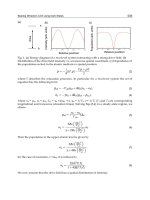
Fig. 4. (a) Schematic diagram illustrating an input field reflected from the back of a
cantilever onto a split detector for position sensing of the tip location with respect to a
sample. The input laser field has a TEM
00
spatial profile, given by v(
ρ
). (b) Sensitivity of (i)
spatial homodyne and (ii) split detection for the measurement of the displacement of a
TEM
00

input field. The local oscillator field had a TEM
10
mode-shape, given by w(
ρ
). (c) The
coefficients of the Taylor expansion of v(
ρ
, p). The coefficients correspond to the undisplaced
(i) TEM
00
, (ii) TEM
10
, (iii) TEM
20
, (iv) TEM
30
, (v) TEM
40
, (vi) TEM
50
modes. Figures (b) and (c)
were reproduced from Hsu et al. (2004), with permission.
4.1 Split detection
We now formalise the effects from the application of split detection in determining the AFM
tip position. We assume that the laser field incident on the AFM cantilever has a TEM
00
Fundamentals and Applications of Quantum Limited Optical Imaging

643
modeshape. The spatial information of the displaced field, reflected from the AFM

cantilever, is described fully by the field operator given in Eq. (1), now expanded to

(29)
where u
mn
(
ρ
, p) are the transverse beam amplitude functions for the displaced TEM
mn
modes
and
δ
mn
are the corresponding quantum noise operators. (p) is the coherent amplitude of
the displaced TEM
00
field. Using the formalism developed in the previous sections, v(
ρ
, p) =
u
00
(
ρ
, p) and substituting this into Eqs. (15) and (16), gives the normalised difference
photocurrent

(30)
where
τ
is the measurement time. The difference photo-current is linearly proportional to

the displacement p. In the regime where the displacement is assumed to be small (whereby
p
w
0
and w
0
is the waist of the incident laser field), the normalised difference photo-current
begins to roll off and asymptotes to a constant for larger p. This can be easily understood,
since for p
w
0
the beam is incident almost entirely on one side of the detector. In this
regime, large beam displacements only cause small variations in 〈Δi
SD
〉, making it difficult to
determine the beam displacement precisely.
For small displacements, the sensitivity of the displacement measurement is found to be
given by (Hsu et al. (2004))

(31)
4.2 Spatial homodyne detection
As discussed earlier, we can use the optimal spatial parameter estimation scheme based on
spatial homodyne detection, to detect the beam position in AFM systems. First, the relevant
signal mode w(
ρ
) of the displaced TEM
00
input field is identified. A Taylor expansion of the
displaced v(
ρ

, p) = u
00
(
ρ
, p) input mode provides the relevant displacement signal mode
w(
ρ
). The coefficients of the Taylor expansion as a function of beam displacement are
illustrated in Fig. 4 (c). For small displacements, only the TEM
00
and TEM
10
modes have
significant non-zero coefficients (Anderson, 1984). This means that for small displacements
the TEM
10
mode contributes most to the displacement signal. For larger displacement, other
higher order modes become significant as their coefficients increase. Therefore a spatial
homodyne measurement of the displaced TEM
00
mode using a LO with centred TEM
10
mode-shape is optimal in the small displacement regime. From Fig. 4 (c), we see that when
the input beam is centred, no power is contained in the TEM
10
mode. Since the Hermite-
Gauss modes are orthonormal, the TEM
10
local oscillator beam only detects the TEM
10

vacuum noise of the input beam. However as the TEM
00
beam is displaced, power is
coupled into the TEM
10
mode. This coupled power interferes with the TEM
10
local oscillator,
causing a linear change in the photo-current observed by the homodyne detector.
Using Eq. (1), the electric field operator describing the TEM
10
local oscillator beam is given by
Advances in Lasers and Electro Optics

644

(32)
where the first bracketed term is the coherent amplitude which resides in the TEM
10
mode,
the second bracketed term denotes the quantum fluctuations of the beam, and
LO
is the
coherent amplitude of the LO. The difference photo-current between the two detectors used
in the spatial homodyne detection can then be shown from Eqs. (21) to be (Hsu et al. (2004))

(33)
where

is the amplitude quadrature noise operator of the TEM

10
component
of the displaced beam, and we have assumed that
LO
(p).
The spatial homodyne detection sensitivity, obtained in the same manner as that for split
detection, is shown in Figure 4 (b). In the small displacement regime, we obtain

(34)
The spatial homodyne detector was shown to be optimal in Section 3.3. Therefore Eq. (34)
sets the optimal sensitivity achievable for small displacement measurements. A comparison
of the efficiency of split detection for small displacement measurement with respect to the
spatial homodyne detector is given by the ratio

(35)
This

factor arises from the coefficient of the mode overlap integral, between v(
ρ
, p) =
u
00
(
ρ
, p) and v
f
(
ρ
, p) = u
f 00

(
ρ
, p), as shown in Eq. (15), where u
f 00
(
ρ
, p) is the flipped TEM
00

mode. Fig. 4 (b) shows that the maximum sensitivity of split detection is limited at ~80 %.
The sensitivity decreases and asymptotes to zero for large displacement, and is below
optimal for all displacement values.
4.3 Using spatial squeezing to enhance measurements for split detection systems
The detection mode arising from the geometry of a split detector is the flipped mode v
f
(
ρ
).
Therefore, in order to perform sub-QNL measurements using a split detector, squeezing of
the flipped mode is required. In the case of a quadrant detector, since both horizontal and
vertical displacements can be monitored, there exist two detection modes. Therefore, two
spatial squeezed modes are required to achieve sub-QNL measurements along two different
axes in the transverse plane. An experimental demonstration of simultaneous squeezing for
quadrant detection along two different axes in the transverse plane was shown by Treps et
al. (2003). In their experiment, three beams were required - a bright coherent field with a
horizontally phase flipped mode-shape, denoted by TEM
f 00
, and two squeezed fields with
TEM
00

and TEM
f 0f 0
(i.e. both phase flipped in the horizontal and vertical axes) mode-shapes,
Fundamentals and Applications of Quantum Limited Optical Imaging

645
as shown in Fig. 5 (a). The mode-shape was obtained via the implementation of phase flips
on the quadrants in the transverse field. These modes were then overlapped using low
finesse, impedance matched optical cavities, with the resulting field imaged onto on a
quadrant detector. Measurements of the beam position fluctuations in the horizontal axis
were performed by taking the difference between the photocurrents originating from the left
and right halves of the quadrant detector. Correspondingly, the beam position fluctuation in
the vertical axis were obtained from the difference of the photocurrents from the top and
bottom halves of the detector. Treps et al. (Treps et al., 2003) demonstrated that simultaneous
sub-QNL fluctuations in both horizontal and vertical beam position are obtainable.


Fig. 5. (a) Schematic of experimental setup for the production of a 2-dimensional spatial
squeezed beam for quadrant detection. (b) Measurements of a displacement signal with
increasing amplitude in time performed using a beam in the (i) coherent state and (ii) spatial
squeezed state. (c) Signal-to-noise ratio (left vertical axis) versus measured displacement.
Traces (iii) and (iv) are results obtained from data traces (i) and (ii), respectively. RBW =
VBW = 1 kHz, averaged over 20 traces each with detection time Δt = 1 ms per data point.
Figures were reproduced from Treps et al. (2002), with permission.
Treps et al. (2003) also showed that simultaneous sub-QNL measurements of a displacement
signal along two different axes can be produced. A displacement modulation at frequency Ω
was applied to the spatial squeezed beam via the use of a mirror mounted on a PZT. The
amplitude of the displacement modulation was determined by demodulating the
photocurrent at frequency Ω and then measuring the power spectral density, using a
spectrum analyser. The measured signal consists of the sum of the squares of the quantum

noise with and without applied displacement modulation, given by p
mod
(Ω) and p
noise
(Ω),
respectively. For a displacement amplitude modulation that increased with time, the results
Advances in Lasers and Electro Optics

646
of the measurement are shown in Fig. 5 (b). Curve (i) is the result of a displacement
measurement performed with a coherent state input beam and sets the classical limit to
displacement measurements using quadrant detectors. Curve (ii) is the result of a
displacement measurement performed using the spatially squeezed beam.
In order to determine the smallest detectable displacement signal, the results obtained were
normalised to the respective noise levels for the coherent and the spatially squeezed beams,
shown in Fig. 5 (c). The vertical axis is the signal-to-noise ratio for the displacement
measurement. With a 99%confidence level, the smallest detectable displacement is 2.3 Å for
a coherent state beam. With the use of the spatially squeezed beam, the smallest detectable
displacement was 1.6 Å. Therefore, the spatial squeezed beam provided a factor of 1.5
improvement in the smallest detectable displacement signal, over the coherent state beam.
4.4 Using spatial squeezing to enhance measurements for spatial homodyne
detection
Although squeezing of the flipped mode v
f
(
ρ
) enhances beam displacement measurements
on a split detector with sensitivity below the QNL, this scheme remains non-optimal for
beam displacement measurements. As shown in previous sections, the QNL for beam
displacement measurements is reached in a spatial homodyne detector, assuming the

imaging field is in the coherent state. Therefore in order to surpass this QNL, squeezing of
the signal mode w(
ρ
) responsible for the beam displacement is required. Following the
theoretical treatment by Hsu et al. (2004), Delaubert et al. (2006) performed the first
experimental demonstration of squeezing the TEM
10
displacement signal mode, for an
incident TEM
00
beam, followed by displacement signal detection using a TEM
10
local
oscillator beam in the spatial homodyne detector.
The squeezed TEM
10
mode of the incident beam was produced by imaging the squeezed
TEM
00
output beam from an optical parametric oscillator (OPO) onto a phase mask, as
shown in Fig. 6 (a). The phase mask converts the TEM
00
squeezed beam into a TEM
10
squeezed beam with an efficiency of ~80 %. By using an asymmetric Mach-Zehnder
interferometer for combining odd and even-ordered modes, the bright TEM
00
beam (i.e.
v(
ρ

)) was combined with the squeezed TEM
10
beam (i.e. w(
ρ
)). The resulting beam was
spatially squeezed for optimal detection of small beam displacements. Using a mirror
actuated via a PZT, displacement of the beam at RF frequencies was imposed. However, this
actuation scheme also introduced a tilt to the beam, therefore the beam was effectively
displaced and tilted in the transverse plane, given by

(36)
where d,
θ
and w
0
are the displacement, tilt and waist of the beam, respectively. The small
beam displacement signal is contained in the amplitude quadrature of the TEM
10
mode,
whilst the small beam tilt signal is contained in the phase quadrature of the TEM
10
mode.
The displacement and tilt of a beam have been shown to be conjugate observables (Hsu et
al., 2005).
The resulting modulated beam was subsequently analysed by interference with a TEM
10
local oscillator beam, produced via an optical cavity resonant on the TEM
10
mode. Note that

Fundamentals and Applications of Quantum Limited Optical Imaging

647

Fig. 6. (a) Schematic diagram of the experimental demonstration of sub-QNL beam
displacement measurement using a spatial homodyne detector. Measurements of the (b)
displacement and (c) tilt modulation signals using a spatial homodyne detector. The tilt
signal was significantly greater than the displacement signal (9:1). Initially the LO and input
beam phases were scanned from 0 to
π
, then was subsequently locked. SQZ: the quadrature
noise for the TEM
10
squeezed mode without modulation signal, resulting in 2 dB of
squeezing and 8 dB of anti-squeezing. MOD: the applied modulation signal detected with
coherent light only. MOD-SQZ: measured modulation signal using TEM
10
squeezed light.
Since the squeezed TEM
10
mode was in-phase with the TEM
00
bright mode component, the
displacement measurement was improved, whilst the tilt measurement was degraded. The
TEM
00
waist size was w
0
=106
μ

min the PZT plane, beam power 170
μ
W, RBW=100 kHz, and
VBW=100 Hz, corresponding to a minimum resolvable displacement QNL of d
QNL
=0.6 nm.
Figures (b) and (c) were reproduced from Delaubert et al. (2006), with permission.

the strength of the spatial homodyne detector is that it can also measure beam tilt, which is
not accessible in the plane of a split detector, simply by adjusting the relative phase between
the LO and the input beams. The resulting interfered beams were then detected on two
photodetectors and their photocurrents analysed on a spectrum analyser. The results are
shown in Fig. 6 (b) and (c), for different relative phase values between the TEM
10
local
oscillator and spatial squeezed beams.
The displacement and tilt of the input beam were accessed by varying the phase of the local
oscillator. When the TEM
10
mode was in phase with the bright TEM
00
mode component,
displacement measurements were enhanced below the QNL, as shown in Fig. 6 (c). Since
beam displacement and tilt are conjugate observables, an improvement in the beam
displacement measurement degraded the tilt measurement, shown in Fig. 6 (b). The
minimum resolvable displacement was d
exp
= 0.15 nm, significantly better than was
achievable without the use of spatially squeezed light.
Advances in Lasers and Electro Optics

648
5. Practical applications 2: Particle sensing in optical tweezers
Optical tweezer systems (Ashkin, 1970) have been used extensively for obtaining
quantitative biophysical measurements. In particular, particle sensing using optical tweezers
provides information on the position, velocity and force of the specimen particles.
A conventional optical tweezers setup is shown in Fig. 7 (a), where a TEM
00
trapping field is
focused onto a scattering particle. The effective restoring/trapping force acting on the
particle is due to two force components: (i) the gradient force F
grad
resulting from the intensity
gradient of the trapping beam, which traps the particle transversely toward the high
intensity region; and (ii) the scattering force F
scat
resulting from the forward-direction


Fig. 7. (a) Illustration showing a TEM
00
trapping field focussed onto a spherical scattering
particle. The gradient and scattering forces are given by F
grad
and F
scat
, respectively. (b)
Schematic representation of the trapping and scattered fields in an optical tweezers. The
trapping field is incident from the left of the diagram. Obj: objective lens, and Img: imaging
lens. (c) Interference pattern of the trapping and forward scattered fields in the far-field

plane. Figures (i)-(iii) and (iv)-(vi) assume that the trapping field is x-and y-linearly
polarised, respectively. The particle displacements are given by (i), (iv): 1
μ
m; (ii), (v): 0.5
μ
m; and (iii), (vi): 0
μ
m. (d) Minimum detectable displacement normalised by K, versus
collection lens NA for (i) split and (ii) spatial homodyne detection. The solid and dashed
lines are for x- and y-linearly polarised trapping fields, respectively. The axis on the right
shows the minimum detectable displacement assuming 200 mW trapping field power,
λ
=
1064 nm, particle radius a = 0.1
μ
m, permittivity of the medium ε
1
= 1, permittivity of the
particle ε
1
= 3.8 and trapping field focus of 4
μ
m. Absorptive losses in the sample were
assumed to be negligible. Figures (b), (c) and (d) were reproduced from Tay et al. (2009),
with permission.
Fundamentals and Applications of Quantum Limited Optical Imaging

649
radiation pressure of the trapping beam incident on the particle. In the focal region of the
trapping field, the gradient force dominates over the scattering force, resulting in particle

trapping.
To obtain a physical understanding of the trapping forces involved, consider the case with a
spherical particle, which has a diameter larger than the trapping field wavelength. Rays 1
and 2 are refracted in the particle, and consequently undergo a momentum change resulting
in an equal and opposite momentum change being imparted on the particle. Due to the in
tensity profile of the beam, the outer ray is less intense than the inner ray which results in
the generation of the gradient force (Ashkin, 1992).
If the particle has radius smaller than the wavelength of the trapping laser however, the
trapping force is instead generated by an induced dipole moment. In this size regime, the
actual shape of the particle is no longer important so long as the particle has no structural
deviations greater than the wavelength of the trapping beam. Hence the particle can be
treated as a normal dipole with an induced dipole moment along the direction of trapping
beam polarisation. The gradient force acting on the particle is then generated due to the
interaction of its induced dipole moment with the transverse electromagnetic fields of the
trapping field. This force is proportional to the intensity of the beam and has the same net
result as before; it acts to return the particle to the centre of the trapping beam focus.
A particle in the beam path will also scatter light. The transverse scattered field profile is
dependent on the position of the particle with respect to the centre of the trapping field. By
imaging the scattered field onto a position sensitive detector, the position and force of the
trapped particle is able to be measured. For these measurements, split detection is most
commonly used (Lang & Block, 2003; Gittes & Schmidt, 1998; Pralle et al., 1999), although
some direct measurement techniques utilise CCD arrays. To demonstrate the potential
enhancement of measurements, we compare split detection and spatial homodyne scheme.
5.1 Modelling
For a single spherical, homogeneous particle with diameter much smaller than the
wavelength, the scattered field can be modelled as dipole radiation (Van de Hulst, 1981)
2
.
The total field after the objective lens consists of both the scattered and residual trapping
fields, given by (Tay et al., 2009)

(37)
where
are the respective complex scattered and trapping fields at the
image plane. To demonstrate how the changing particle position affected the field at the
image plane, Tay et al. (2009) calculated the interference between the forward scattered and
residual trapping fields for a range of particle displacements in the plane of the trap waist,
shown in Fig. 7 (c) for trapping field (i) x- and (ii) y-linearly polarised. Note that the
distribution of the field was compressed in the direction of the trapping field polarisation
due to dipole scattering along the polarisation axis.

2
In the case where there are multiple inhomogeneous particles scattering the input trapping
field, several numerical methods exist to calculate the scattered field - e.g. the finite
difference frequency domain and T-matrix hybrid method (Loke et al., 2007); and the
discrete-dipole approximation and point matching method (Loke et al., 2009).
Advances in Lasers and Electro Optics

650
As before, the critical parameters for assessing sensitivity of particle monitoring are
(p),
v(Γ, p) and w(Γ). Using Eq. (6) we obtain

(38)
where
trap
is the coherent amplitude of the trapping field. Now using Eq. (9) the functional
form for the mode that contains information about the particle position is given by

(39)

Note that this mode is only dependent on the scattered field.
It is then possible to calculate the SNR of the spatial homodyne and split detection schemes
for particle sensing in an optical tweezers arrangement. By substituting the expressions
obtained in Eq. (39) into Eq. (25), the SNR for the spatial homodyne detection scheme is
given by

(40)
where the image plane co-ordinates are given by Γ and

(41)
where ε
1
and ε
2
are the respective permittivity of the medium and particle; and a is the radius
of the particle. In a similar manner, using Eq. (27), the SNR for the split detection scheme is
given by

(42)
Correspondingly, the sensitivities for the spatial homodyne and split detection schemes can
be calculated using Eqs. (26) and (28), respectively. The explicit forms for these expressions
can be found in Tay et al. (2009).
5.2 Results
The performance of both split and spatial homodyne detection schemes were compared by
considering the sensing of particle displacement from the centre of the optical tweezers trap
(Tay et al., 2009). The SNR for (a) split; and spatial homodyne detection in the (b) small and
(c) large displacement regimes are shown in Fig. 8. It was found that the SNR for spatial
homodyne detection was maximised at different particle displacement regimes depending
on the LO mode used.
Fundamentals and Applications of Quantum Limited Optical Imaging

651

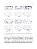
Fig. 8. SNR normalised to K versus particle displacement with respect to the centre of the
trapping field, for (a) split detection; (b) spatial homodyne detection with LO spatial mode
optimised for small displacement measurements; and (c) spatial homodyne detection with
LO spatial mode optimised for larger displacement measurements. The black solid and red
dashed lines are for x- and y-linearly polarised trapping fields, respectively. The
corresponding LO spatial modes are the inset figures with (d) y- and (e) x-linearly polarised
trapping fields for the small displacement regime. For the large displacement regime, the
LO spatial modes are correspondingly: (f) y- and (g) x-linearly polarised trapping fields.
Model parameters are 200 mW trapping field power,
λ
= 1064 nm, particle radius a = 0.1
μ
m,
permittivity of the medium ε
1
= 1, permittivity of the particle ε
1
= 3.8 and trapping field focus
of 4
μ
m. Absorptive losses in the sample were assumed to be negligible. Figures were
reproduced from Tay et al. (2009), with permission.

Assuming small displacements, the LO field was determined from the first order term in the
Taylor expansion of Eq. (9) for the scattered field, with the SNR given in Fig. 8 (b). For
particle displacements less than the trapping beam waist, linearity of the SNR was obtained.
Optimum sensitivity (i.e. the maximum SNR slope) occurred at zero displacement and

surpassed the maximum of split detection by almost an order of magnitude. However, for
particle displacements ~ |0.4j|
μ
m, the SNR peaked, indicating that small displacements of a
particle around ~ |0.4|
μ
m are not resolvable using the current LO mode. As the particle was
displaced further, a drop in the total scattered power was observed due to the particle
moving out of the trapping field, resulting in an exponential decay of the SNR. To re-
optimise the LO mode for particle displacement around any arbitrary position, a Taylor
expansion in p of the scattered field can be taken at that position while only retaining the
first order term. For example, for particles fluctuating around ~ |0.4|
μ
m, the re-optimised
LO mode resulted in the SNR given in Fig. 8 (c) where the maximum SNR slope was now
located around ~ ±0.4
μ
m. Therefore, it is possible to dynamically adjust the LO mode to
optimise the measurement sensitivity whilst the particle moves, resulting in optimum
particle sensing for all displacement values.
The corresponding sensitivities for (i) split and (ii) spatial homodyne detection as a function
of increasing objective lens NA are shown in Fig. 7 (d). It was observed that the minimum
detectable displacement for both split and spatial homodyne detection decreased with
increasing NA due to more scattered field being collected, thereby providing more
information about the particle position. However, spatial homodyne detection outperforms
split detection for all NA values, since spatial homodyne optimally extracts the
displacement information from the detected field, whereas the split detection scheme only
measures partial displacement information, as shown in Eq. (15). Due to the optimal signal
Advances in Lasers and Electro Optics

652
and noise measurement using the spatial homodyne scheme, curve (ii) defines the minimum
detectable displacement in optical tweezers systems.
To provide quantitative values for the minimum detectable displacement, the sensitivities
for both detection schemes using realistic experimental values are shown in the right-hand
side axis of Fig. 7 (d). The split detection non-optimality shaded area shows the loss in particle
sensing sensitivity due to incomplete mode detection from a split detector. The quantum
resources shaded area shows that quantum resources such as spatial squeezed light (Treps et
al., 2002; 2003) can be used to further enhance the particle sensing sensitivity beyond the
QNL.
The ability to tailor the local oscillator mode provides tremendous optimisation ability for
particle sensing. Not only is optimal information extraction possible, but it is now possible
to perform sensing of multiple inhomogeneous particles, with information extraction of any
spatial parameter p, via the modification of the LO mode.
6. Conclusion
We have presented a quantum formalism for the measurement of the spatial properties of
an optical field. It was shown that the spatial homodyne technique is optimal and
outperforms split detection for the detection of spatial parameter p. Applications of this
measurement scheme in enhancing the sensitivities of atomic force microscopes and optical
tweezers measurements have been discussed.
7. References
Anderson, D. Z. (1984). Alignment of resonant optical cavities. Appl. Opt., Vol. 23, No. 17,
2944-2949.
Arnon, S. (1998). Use of satellite natural vibrations to improve performance of free-space
satellite laser communication. Appl. Opt., Vol. 37, 5031.
Ashkin, A. (1992). Forces of a single-beam gradient laser trap on a dielectric sphere in the
ray optics regime. Biophys. J., Vol. 61, No. 2, 569–582.
Ashkin, A. (1970). Acceleration and Trapping of Particles by Radiation Pressure. Phys. Rev.
Lett Vol. 24, No. 4, 156-159.
Beck M. (2000). Quantum state tomography with array detectors Phys. Rev. Lett., Vol. 84, No.

25, 5748.
Binnig, G.; Quate, C. F.; and Gerber, Ch. (1985). Atomic Force Microscope. Phys. Rev. Lett.,
Vol. 56, No. 9, 930-933.
Block S. M. (1992). Making light work with optical tweezers Nature, Vol. 360, 493-495.
Born M. and Wolf E. Principles of Optics (Cambridge University Press, Cambridge, UK, 1999)
Bowen W. P., Schnabel R., Bachor H A. , and Lam P. K. (2002). Polarization squeezing of
continuous variable stokes parameters. Physical Review Letters Vol. 88, 093601.
Dawes, A.M.; Beck, M.; and Banaszek, K. (2003). Mode optimization for quantum-state
tomography with array detectors. Phys. Rev. A., Vol. 67, 032102.
Dawes, A.M.; and Beck, M. (2001). Simultaneous quantum-state measurements using array
detection. Phys. Rev. A., Vol. 63, 040101(R).
Delaubert, V., Treps, N., Harb, C. C., Lam, P. K., and Bachor, H A. (2006). Quantum
measurements of spatial conjugate variables: displacement and tilt of a Gaussian
beam. Opt. Letts., Vol. 31, No. 10, 1537-1539.
Fundamentals and Applications of Quantum Limited Optical Imaging

653
Delaubert, V.; Treps, N.; Fabre, C.; Bachor, H A.; and R´efr´egier, P. (2008). Quantum limits
in image processing. Europhys. Lett., Vol. 81, 44001.
Fabre, C.; Fouet, C. J.; and Maˆıtre, A. (2000). Quantum limits in the measurement of very
small displacements in optical images. Opt. Lett., Vol. 25, pp. 76.
Fritschel, P.; Mavalvala, N.; Shoemaker, D.; Sigg, D.; Zucker, M.; and González, G. (1998).
Alignment of an interferometric gravitational wave detector. Appl. Opt., Vol. 37,
No. 28, 6734–6747.
Fritschel, P.; Bork, R.; Gonz´alez, G.; Mavalvala, N.; Ouimette, D.; Rong, H.; Sigg, D.; and
Zucker, M. (2001). Readout and Control of a Power-Recycled Interferometric
Gravitational-Wave Antenna. Appl. Opt., Vol. 40, No. 28, 4988–4998.
Gittes, F.; and Schmidt, C. F. (1998). Interference model for back-focal-plane displacement
detection in optical tweezers. Opt. Lett. Vol. 23, No. 1, 7–9.
Hell, S.W.; Schmidt, R.; and Egner, A. (2009). Diffraction-unlimited three-dimensional

optical nanoscopy with opposing lenses Nature Photonics 3, 381-387.
Hsu, M. T. L.; Delaubert, V.; Lam, P. K.; and Bowen,W. P. (2004). Optimal optical
measurement of small displacements. Journal of Optics B:Quantum and Semiclassical
Optics, Vol. 6, No. 12, 495-501.
Hsu, M. T. L.; Bowen, W. P.; Treps, N.; and Lam, P. K. (2005). Continuous-variable spatial
entanglement for bright optical beams. Phys. Rev. A, Vol. 72, No. 1, 013802.
Hsu, M. T. L.; Bowen,W. P. and Lam, P. K. (2009). Spatial-state Stokes-operator squeezing
and entanglement for optical beams. Physical Review A, Vol. 79, No. 4, 043825.
Korolkova, N. V.; and Chirkin, A. S. (1996). Formation and conversion of the polarization-
squeezed light. Journal of Modern Optics, Vol. 43, issue 5, 869-878.
Lang, M. J.; and Block, S. M. (2003). LBOT-1: Laser-based optical tweezers. Am. J. Phys., Vol.
71 No. 3, 201–215; and references therein.
Loke, V. L. Y.; Nieminen, T. A.; Parkin, S. W.; Heckenberg, N. R.; and Rubinsztein-Dunlop,
H. (2007). FDFD/T-matrix hybrid method. J. Quant. Spec. Rad. Trans., Vol. 106, No.
1, 274–284.
Loke, V. L. Y.; Nieminen, T. A.; Heckenberg, N. R.; and Rubinsztein-Dunlop, H., J. (2009). T-
matrix calculation via discrete dipole approximation, point matching and
exploiting symmetry. Quant. Spec. Rad. Trans., Vol. 110, No. 14, 1460–1471.
Mach, L. (1892). Z. Instrumentenkunde 12, 89.
Nikulin, V. V.; Bouzoubaa, M.; Skormin, V. A.; and Busch, T. E. (2001). Modeling of an
acousto-optic laser beam steering system intended for satellite communication. Opt.
Eng., Vol. 40, 2208.
Pawley J. (1995). Handbook of Biological Confocal Microscopy, Springer, Germany.
Pendry, J. B. (2000). Negative refraction makes a perfect lens. Phys. Rev. Lett. , Vol. 85, No. 14,
3966-3969.
Pralle, A.; Prummer, M.; Florin, E L.; Stelzer, E. H. K.; and Hörber, J. K. H. (1999).
Threedimensional high-resolution particle tracking for optical tweezers by forward
scattered light. Microsc. Res, Tech., Vol. 44, No. 5, 378-386.
Putman, C. A.; De Grooth, B. G.; Van Hulst, N. F.; and Greve, J. (1992). A detailed analysis of
the optical beam deflection technique for use in atomic force microscopy. J. Appl.

Phys., Vol. 72, No. 1, 6.
Sagnac, G. (1912). L’éther lumineux démontré par l’effet du vent relatif d’éther dans un
interférométre en rotation uniforme. Comptes Rendus 157 (1913), S. 708-710
Advances in Lasers and Electro Optics

654
Saleh, B. E. A.; and Teich, M. C. (1991). Fundamentals of Photonics, JohnWiley and Sons,
New York.
Shaddock, D. A.; Gray, M. B.; and McClelland, D. E., (1999). Frequency locking a laser to an
optical cavity by use of spatial mode interference. Opt. Lett., Vol. 24, No. 21, pp.
1499-1501.
Slusher, R. E.; Hollberg, L. W.; Yurke, B.; Mertz, J. C.; and Valley, J. F. (1985). Observation of
Squeezed States Generated by Four-Wave Mixing in an Optical Cavity, Phys. Rev.
Lett., Vol. 55, No. 22, 2409-2412.
Synge, E. H. (1928). A suggested method for extending the microscopic resolution into the
ultramicroscopic region. Phil. Mag. 6, 356.
Tay, J. W.; Hsu, M. T. L.; and Bowen, W. P. (2009). Quantum limited particle sensing in
optical tweezers. e-print arXiv:0907.4198
Treps, N.; Andersen, U.; Buchler, B.; Lam, P. K.; Maˆıtre, A.; Bachor, H A.; and Fabre, C.
(2002). Surpassing the Standard Quantum Limit for Optical Imaging Using
Nonclassical Multimode Light. Phys. Rev. Lett., Vol. 88, No. 20, 203601 (2002).
Treps, N., Grosse, N.; Bowen,W. P.; Fabre, C.; Bachor, H A.; and Lam, P. K. (2003). A
Quantum Laser Pointer. Science., Vol. 301, No. 5635, 940–943. See also: Treps, N.;
Grosse, N.; Bowen, W. P.; Hsu, M. T. L.; Maître, A.; Fabre, C.; Bachor, H A.; and
Lam, P. K. (2004). Nano-displacement measurements using spatially multimode
squeezed light. J. Opt. B: Quantum Semiclass., Vol. 6, No. 8, S664–S674.
Treps, N.; Delaubert, V.; Maître A.; Courty, J.M.; Fabre, C. (2005). Quantum noise in
multipixel image processing. Phys. Rev. A, Vol. 71, No. 1, 013820.
Van De Hulst, H. C. (1981). Light Scattering by Small Particles. Dover Publications,
ISBN:0486642283, New York. See also: Berne, B. J., and R. Pecora. (2000). Dynamic

Light Scattering. Dover Publications, ISBN:0486411559, New York.
Walls, D. F.; and Milburn, G. J. (1995). Quantum Optics, Springer, Germany. Zehnder, L.
(1891). Z. Instrumentenkunde 11, 275.
28
Broadband Light Generation
in Raman-active Crystals Driven by
Femtosecond Laser Fields
Miaochan Zhi, Xi Wang and Alexei V. Sokolov
Texas A&M University
U. S. A
1. Introduction
Short pulse generation requires a wide phase-locked spectrum. Earlier the short pulses were
obtained by expanding the spectrum of a mode locked laser from self phase modulation
(SPM) in an optical fiber and then compensating for group velocity dispersion (GVD) by
diffraction grating and prism pairs. Pulses as short as 4.4 fs have been generated
(Steinmeyer et al., 1999). For ultrafast measurements on the time scale of electronic motion,
generation of subfemtosecond pulses is needed. Generation of subfemtosecond pulses with
a spectrum centered around the visible region is even more desirable, due to the fact that the
pulse duration will be shorter than the optical period and will allow sub-cycle field shaping.
As a result, a direct and precise control of electron trajectories in photoionization and high-
order harmonic generation will become possible. But to break the few-fs barrier new
approaches are needed.
In recent past, broadband collinear Raman generation in molecular gases has been used to
produce mutually coherent equidistant frequency sidebands spanning several octaves of
optical bandwidths (Sokolov & Harris, 2003). It has been argued that these sidebands can be
used to synthesize optical pulses as short as a fraction of a fs (Sokolov et al., 2005). The
Raman technique relied on adiabatic preparation of near-maximal molecular coherence by
driving the molecular transition slightly off resonance so that a single molecular
superposition state is excited. Molecular motion, in turn, modulates the driving laser
frequencies and a very broad spectrum is generated, hence the term for this process

“molecular modulation”. By phase locking, a pulse train with a time interval of the inverse
of the Raman shift frequency is generated. While at present isolated attosecond X-ray pulses
are obtained by high harmonic generation (HHG) (Kienberger et al., 2004), the pulses are
difficult to control because of intrinsic problems of X-ray optics. Besides, the conversion
efficiency into these pulses is very low (typically 10
−5
). On the other hand, the Raman
technique shows promise for highly efficient production of such ultrashort pulses in the
near-visible spectral region, where such pulses inevitably express single-cycle nature and
may allow non-sinusoidal field synthesis (Sokolov et al., 2005).
In the Raman technique ns pulses are applied for preparing maximal coherence when gas is
used as a Raman medium. When the pulse duration is shorter than the dephasing time T
2

Advances in Lasers and Electro Optics

656
(

is the Raman linewidth), the response of the medium is a highly transient
process, i.e. the Raman polarization of the medium doesn’t reach a steady state within the
duration of the pump pulse. In this transient stimulated Raman scattering (SRS) regime, a
large coherent molecular response is excited. The advantage of using a short pulse is that the
number of pulses in the train will be reduced compared with the ns Raman technique. But
when a single fs pump is used, the strong SPM suppresses the Raman generation (Kawano
et al., 1998). When the pulse duration is reduced to less than a single period of molecular
vibration or rotation, an impulsive SRS regime is reached (Korn et al., 1998). In this regime,
an intense fs pulse with a duration shorter than the molecular vibrational period prepares
the vibrationally excited state and a second, relatively weak, delayed pulse propagates in
the excited medium in the linear regime and experiences scattering due to the modulation of

its refractive index by molecular vibrations, which results in the generation of the Stokes
and anti-Stokes sidebands (Nazarkin et al., 1999). This technique has the advantage of
eliminating the parasitic nonlinear processes since they are confined only within the pump
pulse duration.
A closely related approach, which is called four-wave Raman mixing (FWRM) for
generating ultrashort pulses using two-color stimulated Raman effect, is proposed by
Imasaka (Yoshikawa & Imasaka, 1993). It is based on an experimental result his student has
stumbled on. Shuichi Kawasaki was trying to develop a tunable source for thermal lens
spectroscopy and he noticed bright, multicolored spots out of the Raman cell pressurized
with hydrogen, which they called “Rainbow Star” (Katzman, 2001). The applied beam was
supposed to be monochromatic but it actually had two colors in it. To confirm the FWRM
hypothesis, a nonlinear optical phenomenon in which three photons interact to produce a
fourth photon, they used two-color laser beams with frequencies separated by one of the
rotational level splitting for hydrogen (590 cm
−1
). Indeed, they observed the generation of
more than 40 colors through the FWRM process, which provided a coherent beam consisting
of equidistant frequencies covering more than thousandths cm
−1
in frequency domain
(Imasaka et al., 1989). This FWRM process resulted in the generation of higher-order
rotational sidebands at reduced pump intensity compared to the stimulated Raman
scattering. The generation of the FWRM fields required phase matching and were
coherently phased, and therefore had the potential to be used to generate sub-fs pulses
(Kawano et al., 1999).
Later ps pulses (Kawano et al., 1996), ps and fs pump pulses (Kawano et al., 1997), and a
single fs pulse (Kawano et al., 1998) were used to find the optimal experimental conditions
for efficient generation of high-order rotational lines. Generally speaking, when the
additional Stokes field is supplied rather than grown from quantum noise, advantages
include: highorder anti-Stokes generation, higher conversion efficiency, and improved

reproducibility of the pulses generated, as shown in earlier experiments with gas in ns
regime (Gathen et al., 1990). Recently, efficient generation of high-order anti-Stokes Raman
sidebands in a highly transient regime is also observed using a pair of 100-fs laser pulses
tuned to Raman resonance with vibrational transitions in methane or hydrogen (Sali et al.,
2004; 2005). They found that in this transient regime, the two-color set-up permits much
higher conversion efficiency, broader generated bandwidth, and suppression of the
competing SPM. The high conversion efficiency observed proves the preparation of
substantial coherence in the system although the prepared coherence in the medium cannot
be near maximal as in the case of the adiabatic Raman technique.
Broadband Light Generation in Raman-active Crystals Driven by Femtosecond Laser Fields

657
Almost all these works were carried out using a simple-molecule gas medium such as H
2
,
D
2
, SF
6
or methane since the gas has negligible dispersion and long coherence lifetime.
Molecular gas also has a few other advantages as a Raman medium. They are easily
obtainable with a high degree of optical homogeneity and have high frequency vibrational
modes with small spectral broadening, which leads to large Raman frequency shifts and
large Raman scattering cross sections. However, a Raman gas cell with long interaction
length is needed due to the lower particle concentration (Basiev & Powell, 1999).
What about a solid Raman medium such as a Raman crystal? As we know, the high density
of solids results in the high Raman gain. The higher peak Raman cross sections in crystals
result in lower SRS thresholds, higher Raman gain, and greater Raman conversion efficiency
(Basiev & Powell, 1999). In addition, there is no need for cumbersome vacuum systems
when working with room temperature crystals, and therefore a compact system can be

designed.
The difficulty in using crystals is the phase matching between the sidebands because the
dispersion in solids is significant. Sideband generation using strongly driven Raman
coherence in solid hydrogen is reported but the generation process is very close to that of H
2
gas and solid hydrogen is a very exotic material (Liang et al., 2000). Observation of
generation with few sidebands (Stokes or anti-Stokes) in other solid material is nothing new.
About two decades ago, Dyson et. al. has observed one Stokes (S) and one anti-Stokes (AS)
generated on quartz during an experiment designed for another purpose (Dyson et al.,
1989). Later, there were numerous works of using Raman crystals for building Raman lasers
which extended the spectral coverage of solid-state lasers by using SRS (Pask, 2003). A
detailed review of crystalline and fiber Raman lasers is given by Basiev (Basiev et al., 2003).
The focus of our work is efficient generation over a broad spectral range. Compared to the
crystals that are used for building Raman lasers, the sample we use is much thinner (about 1
mm or less). The phenomenon that we use in our work is essentially different from SRS: in
our regime the generation process is fully coherent, does not depend on seeding by
spontaneous scattering, and occurs on a time scale much shorter than the inverse Raman
linewidth. We use two-color pumping (with the frequency difference matching the Raman
frequency), so our sideband generation is more similar to multiple-order coherent Anti-
Stokes Raman Scattering (CARS) than to SRS.
Therefore this chapter is focused on the development of efficient broadband generation
using Raman crystals. Since coherence lifetime in a solid is typically shorter than in a gas,
the use of fs (or possibly ps) pulses is inevitable when working with room-temperature
solids. We studied broadband sideband generation in a Raman-active crystal lead tungstate
(PbWO
4
) either with two 50 fs pulses or a pair of time-delayed chirped pulses (Zhi &
Sokolov, 2007; 2008). Similar broadband generation is also observed in diamond (Zhi et al.,
2008). Coherent high-order anti-Stokes scattering has also been observed in many other types
of crystals such as YFeO

3
, KTaO
3
, KNbO
3
and TiO
2
when two-color femtosecond (fs) pulses are
used (Takahashi, 2004; Matsubabra et al., 2006; Matsuki et al., 2007). Great progress has been
made recently toward synthesis of ultrashort, even few-cycle pulses using Raman crystal. For
example, last year Matsubara et al. have demonstrated promising Fourier synthesizer using
multiple CARS signals obtained in a LiNbO
3
crystal at room temperature, and generated
isolated pulses with 25 fs duration at 1 kHz repetition rate (Matsubara et al., 2008). Very
recently, they just realized the generation of pulses in the 10 fs regime using multicolor
Raman sidebands in KTaO
3
(Matsubara et al., 2009).