Advances in Solid State Part 7 potx
Bạn đang xem bản rút gọn của tài liệu. Xem và tải ngay bản đầy đủ của tài liệu tại đây (1.85 MB, 30 trang )
Continuous-Time Analog Filtering: Design Strategies and Programmability
in CMOS Technologies for VHF Applications
171
control the HS transconductance from 270 to 452 μA/V, and changes from 40 to 100 μA in
the FC topology control the transconductance from 550 to 800 μA/V.
200
250
300
350
400
450
-450 -350 -250 -150 -50 50 150 250 350 450
V
c
(mV)
IBIAS=180uA
IBIAS=135uA
IBIAS=90uA
IBIAS=45uA
480
520
560
600
640
680
720
760
800
-140 -105 -70 -35 0 35 70 105 140
V
c
(mV)
IBIAS=100uA
IBIAS=80uA
IBIAS=60uA
IBIAS=40uA
(a) (b)
Fig. 15. Transconductance versus biasisng currents (fine tuning) for the: (a) HS
implementation; (b) FC implementation.
To conclude, the proposed structure is a balanced topology aimed at improving immunity
to digital noise and linearity. A digitally programmable transconductor has been designed,
maintaining the same dynamic range over the entire frequency range. Therefore, it can be
used in the design of programmable filters, as the expected characteristics of a
programmable cell will be obtained: to maintain Q-factor, noise power and maximum signal
swing constant over the entire programming range, leading to a DR independent on the
operation frequency. The expected linear dependence of the unity-gain frequency is
obtained and the phase error is effectively reduced over the entire programming range in
both implementations, with a compensation scheme based on two cross-coupled capacitors
for the HS topology and the classical RC circuit connected at the input for the FC approach.
8. Results and discussion
To demonstrate the theoretical advantages of this approach for a programmable
transconductor suitable for VHF, two 3-bit programmable integrators have been designed.
The HS transconductor has been implemented by using the design kit of an AMI
Semiconductor (AMIS) 0.35 μm CMOS technology (P-substrate, N-well, 5-metal, 2-poly)
with a 3 V power supply and a nominal bias current of 90 μA per branch; whereas the FC
transconductor has been implemented by using the design kit of an AMS (C35B4C3) 0.35 μm
CMOS technology (P-substrate, N-well, 4-metal, 2-poly) with a 2 V power supply and a
nominal bias current of 100 μA per branch.
The dimensions of the transistors were chosen in order to cover all the design requirements
obtained in this chapter, leading to a complete sweep of the discrete step by varying the bias
current. In this way, for the HS implementation, the operation point is located at 90 μA and
the bias current adjustment is possible from 45-180 μA. However, for the FC
implementation, the operating point is located at 100 μA, covering the digital step by
varying the bias current from 20-110 μA. In this way, the discrete tunability requirement is
obtained but the FC transconductance value at the operation point is maximised.
8.1 Layout strategy
A careful layout has been drawn out to obtain all the characteristics associated with the
proposed design accurately and demonstrate the feasibility of the intended approach. As
g
m
(μA/V)
g
m
(μA/V)
Advances in Solid State Circuits Technologies
172
stated below, we have taken special care to get rid of the unwanted effects related to
parasitic elements and mismatching (Baker et al., 1998; Hastings, 2001). All the designs have
been carried out taking into account the specific design rules for high frequency operation,
which are highly appropriate for obtaining good matching between components.
Interdigitized and common-centroid layout techniques have been considered to reduce the
variations of threshold voltage, which are associated with gradients in gate-oxide thickness.
Guard rings have been included in the design with the aim of reducing substrate noise.
Bond-pads have also been carefully laid out and, in this way, input and output pins have
been placed as far as possible between them. Balanced structures provide outstanding
benefits, but they are strongly dependent on the symmetry of the circuit. Consequently,
special care has been taken to outline the paths of the balanced signals, in an attempt to
ensure the best matching between them. MOS devices have fragile gates seeing that
electrostatic discharges may cause destruction of the device if the oxide breakdown voltage
is exceeded. Considering this point, we concluded that it would be advisable to provide the
transistors that control the quality factor of the circuit with a path protection system. The
scheme chosen to achieve this goal was the anti-parallel diodes configuration. This circuit is
very straightforward and simple but is sufficient for the purposes of this work.
Fig. 16(a) shows the drawn layout of the HS test chip with an active area of 0.10 mm
2
. Fig.
16(b) shows the microphotograph of the programmable FC transconductor, with an active
area of 0.04 mm
2
including the compensation RC circuit, where the integration capacitance
has been implemented with a double-poly capacitor. The area of the FC active element is
0.03 mm
2
and a regular and compact arrangement of transistors can be observed.
(a) (b)
Fig. 16. (a) Layout of the fully-balanced 3-bit programmable HS integrator.
(b) Microphotograph of the FC integrator, by using double-poly capacitors.
8.2 Experimental results
For the HS approach, a unity-gain frequency of 28 MHz was achieved with a power
dissipation of 1.62 mW using a 3 V supply. By varying the digital word from 1 to 7, we
expected to control the unity-gain frequency from 28 to 185 MHz and the experimental
results lead to a variation between 25 and 185 MHz, as shown in Fig. 17(a). Focusing on the
b
2
b
1
b
0
Continuous-Time Analog Filtering: Design Strategies and Programmability
in CMOS Technologies for VHF Applications
173
same figure, by varying the bias current source from 45 to 180 μA for a fixed digital word,
the transconductance value is modified, providing complementary fine tuning of the
frequency. All discrete steps are covered and, in consequence, a frequency span of 25-185
MHz can be provided. The maximum frequency error is obtained at the maximum digital
word where a deviation of 6 % is obtained from the 7:1 ratio.
10
50
90
130
170
210
250
290
45 65 85 105 125 145 165 185
7gm
6gm
5gm
4gm
3gm
2gm
1gm
20
40
60
80
100
120
140
160
180
200
220
20 30 40 50 60 70 80 90 100 110
5gm
4gm
3gm
2gm
1gm
(a) (b)
Fig. 17. Experimental results for coarse and fine tuning of the (a) HS and (b) FC topology.
Variation of the unity-gain frequency versus bias currents for all the digital words.
For the FC approach, a unity-gain frequency of 40 MHz is achieved with a power
dissipation of 2.4 mW using a 2 V supply, as expected from the post-layout simulation
results. By varying the digital word from 1 to 5, the unity-gain frequency is controlled from
40 to 190 MHz, as shown in Fig. 17(b). All discrete steps are swept by varying the bias
current from 20 to 110 μA. The maximum frequency error is obtained at the maximum
digital word where a deviation of 5 % is obtained from the 5:1 ratio.
The next step is to demonstrate constant linearity by means of a constant THD over the
entire programming range. Figs. 18 and 19 show the THD variation as a function of the
differential output current for all the digital words. THD was measured for a sine input
current of 10 MHz (a) and for the unity-gain frequency (b) in both topologies. These figures
show the expected THD dependence, studied above in section §6: lower bias currents or
higher input signal amplitudes lead to higher THD values. A corner parameter analysis was
carried out following the guidelines provided by the design kit manufacturer of the ‘AMI
Semiconductor C035M Design-Kit’ and the worst-case analysis for the HS integrator was
obtained. This distortion study gave 1 % of THD for a differential input signal of 56 μA and
10 MHz. Experimental results for the design, shown in Fig. 18, lead to a differential input
current of 50 μA in the same situation. For the FC approach, the expected value for 1 % of
THD was a differential input signal amplitude of 37 μA and 10 MHz; and the experimental
results (Fig. 19), give an amplitude of 35 μA.
The post-layout simulated result for the input-referred noise integrated from 0 to 30 MHz in
the HS topology was 11.2 nA
rms
. Hence, the dynamic range, defined as the input signal
amplitude at 1 % THD divided by the total noise level integrated over 30 MHz, is 70 dB. In
the FC structure, the input-referred noise integrated from 0 to 40 MHz was 8 nA
rms
. Hence,
the dynamic range, defined as the input signal amplitude at 1 % THD divided by the total
noise level integrated over 40 MHz, is also 70 dB.
In summary, frequency is adjusted in a coarse discrete way by connecting identical
transconductors in parallel and with fine continuous tuning by varying the biasing current.
ω
t
(MHz)
I
bias
(
μ
A)
ω
t
(MHz)
I
bias
(
μ
A)
Advances in Solid State Circuits Technologies
174
-60
-56
-52
-48
-44
-40
-36
0 0,04 0,08 0,12 0,16 0,2 0,24 0,28
iout/Ibias
THD(dB) @ 10MHz
4gm
2gm
gm
-70
-65
-60
-55
-50
-45
-40
-35
0,04 0,12 0,20 0,28 0,36 0,44
iout/Ibias
THD(dB) @ Wt=25 MHz
4gm
2gm
gm
(a) (b)
Fig. 18. THD versus differential output current in the HS integrator for three different digital
words: (a) ω(input)=10 MHz, (b) ω(input)= ω
t
(25 MHz for 1g
m
).
-65
-60
-55
-50
-45
-40
-35
0,04 0,08 0,12 0,16
iout/Ibias
THD(dB) @ 10 MHz
gm
2gm
3gm
4gm
5gm
-65
-60
-55
-50
-45
-40
-35
0,04 0,08 0,12 0,16 0,2 0,24
iout/Ibias
THD(dB) @ Wt=40 MHz
gm
2gm
3gm
4gm
5gm
(a) (b)
Fig. 19. THD versus differential output current in the FC integrator for all the digital words:
(a) ω(input)=10 MHz, (b) ω(input)= ω
t
(40 MHz for 1g
m
).
The feasibility of the programmable array of transconductors has been proven in a 3-bit
programmable integrator obtaining frequency scaling as expected. All the specifications in
both transconductor implementations are summarized in table 7. The main advantage of the
topology proposed was the inherent enhancement of the dc-gain, provided through the
existing positive feedback compensation (negative resistance).
The HS design condition was very difficult to achieve because technological process and
temperature variations are expected to be greater than the small changes required in this
topology. As expected, by varying the external control for this negative resistance, no
change was obtained for the dc-gain. The post-layout simulated dc-gain was a variation of
15 dB between the minimum (40 dB) and the maximum (55 dB), with a maximum CMRR of
60 dB. The experimental results lead to a differential dc-gain of 30 dB with no change with
the value of the negative resistance and a CMRR greater than 35 dB over the entire
frequency range. Therefore, in this case, there is no control on the dc-gain of the system.
The design condition for the FC topology is less restrictive and two different
implementations have been fabricated. The post-layout simulation results in both cases
showed a dc-gain control of 15 dB from 30 to 45 dB and a maximum CMRR of 50 dB. The
first implementation has been designed with the same dimensions for the M
N
transistors
Continuous-Time Analog Filtering: Design Strategies and Programmability
in CMOS Technologies for VHF Applications
175
involved in the negative resistance, and similar results are obtained as in the HS topology.
There is no external dc-gain control and an experimental value of 26 dB and CMRR of 33 dB
are obtained. In the second one, where a pre-designed mismatching is included between M
N
transistors involved in the negative resistance, a variation of 12 dB (from 26 to 38 dB) for the
dc-gain is obtained by modifying the value of the negative resistance (Fig. 20). The CMRR is
greater than 46 dB over the entire frequency range.
HS topology FC topology
Power supply voltage 3 V 2 V
Unity-gain frequency 25 MHz 40 MHz
Power dissipation 1.62 mW 2.4 mW
CMRR over the entire pass-band >35 dB >46 dB
Active area 0.10 mm
2
0.04 mm
2
Total rms input-referred noise (sim.) 11.2 nA
rms
8 nA
rms
Maximum differential input signal
current at 1 % THD @ 10 MHz
50 μA (peak) 35 μA (peak)
Dynamic range 70 dB 70 dB
Table 7. Summary of the experimental results for the integrator (1 LSB).
-25
-15
-5
5
15
25
35
0 1 10 100 1000
frequency ( MHz)
gain (dB)
Fig. 20. Experimental dc-gain control for the FC transconductor with a pre-designed
mismatching between M
N
transistors involved in the negative resistance.
9. Conclusion
This work describes a new approach for implementing digitally programmable and
continuously tunable VHF/UHF transconductors compatible with pure digital CMOS
technologies and suitable for HDD read channel applications. The cell is suitable for low-
voltage operation over an extended frequency range. The programmability exhibited by the
transconductor is due to the use of a generic programmable structure that gives a G
m
digital
control as a parallel connection of unit cells, and the total parasitic capacitances are
maintained constant thanks to the specific design of the unit cell: a cascode stage with
12 dB
Advances in Solid State Circuits Technologies
176
dummy elements. This transconductor could be used in any kind of G
m
-C filter, thus
providing a very wide range of programmable CT filters. The fully-balanced current-mode
G
m
-C integrator based on this topology exhibits a unity-gain frequency programmability
from 25-185 MHz in the HS implementation and 40-200 MHz in the FC approach; with a
phase error of less than 4º in both topologies throughout the entire operating frequency
range. Total harmonic distortion (THD) of less than 1 % (-40 dB) for a differential input
signal of 50 and 35 μA in the HS and FC topology respectively is obtained. The integrator
operates over the programming range with 70 dB of dynamic range for 1 % of THD. The cell
has been fabricated in a 0.35 μm CMOS process.
The experimental results confirm this approach as an excellent choice to achieve filters
exhibiting a good trade-off between tuning capability and dynamic range working in the
very high frequency range. The proposed technique can be easily adapted to lower power
supply voltages by using folded cascode structures and, in addition, better frequency ranges
of operation can be achieved considering current CMOS digital technologies.
10. References
Abidi A. (1988). On the Operation of Cascode Gain Stages. IEEE Journal of Solid-State Circuits,
Vol. 23, No. 6, 1988, 1434-1437, ISSN: 0018-9200.
Ahn H.T. & Allstot D. J. (2002). A 0.5-8.5 GHz Fully-Differential CMOS Distributed
Amplifier. IEEE Journal of Solid-State Circuits, Vol. 37, No. 8, August 2002, 985-988,
ISSN: 0018-9200.
Baker R.J.; Li H.W. & Boyce D.E. (1998). CMOS Circuit Design, Layout and Simulation. IEEE
Press Series on Microelectronic Systems, 1998.
Baschirotto A.; Rezzi F. & Castello R. (1994). Low-Voltage Balanced Transconductor with
High Input Common-Mode Rejection. Electronics Letters, Vol. 30, No. 20, September
1994, 1669-1671, ISSN: 0013-5194.
Bollati G.; Marchese S.; Demicheli M. & Castello R. (2001). An Eight-Order CMOS Low-Pass
Filter with 30-120 MHz Tuning Range and Programmable Boost. IEEE Journal of
Solid-State Circuits, Vol. 36, No. 7, July 2001, 1056-1066, ISSN: 0018-9200.
Croon J.A.; Rosmeulen M.; Decoutere S.; Sansen W. & Maes H.E. (2002). An Easy-to-Use
Mismatch Model for the MOS Transistor. IEEE Journal of Solid-State Circuits, Vol. 37,
No. 8, August 2002, 1056-1064, ISSN: 0018-9200.
Felt E.; Narayan A. & Sangiovanni-Vincentelli A. (1994). Measurement and Modelling of
MOS Transistors Current Mismatch in Analog ICs, Proceedings of the IEEE/ACM
International Conference on Computer Aided Design, pp. 272-277, ISBN: 0-8186-6417-7,
San Jose, California, November 1994, Broadway, New York.
Gray P.R. & Meyer R.G. (2001). Analysis and Design of Analog Integrated Circuits, 4
th
Edition,
John Wiley & Sons, Inc., 2001.
Gregor R.W. (1992). On the Relationship Between Topography and Transistor Matching in
an Analog CMOS Technology. IEEE Transactions on Electron Devices, Vol. 39, No. 2,
1992, 275-282, ISSN: 0018-9383.
Hastings A. (2001). The Art of Analog Layout, Prentice Hall, Inc., 2001.
Continuous-Time Analog Filtering: Design Strategies and Programmability
in CMOS Technologies for VHF Applications
177
Mohan S.S.; Hershenson M.; Boyd S.P. & Lee T.H. (2000). Bandwidth Extension in CMOS
with Optimized On-Chip Inductors. IEEE Journal of Solid-State Circuits, Vol. 53, No.
3, March 2000, 346-355, ISSN: 0018-9200.
Nauta B. (1993). Analog CMOS Filters for Very High Frequencies, Kluwer Academic Publishers,
1993.
Otín A.; Celma S. & Aldea C. (2004). Digitally Programmable CMOS Transconductor for
Very High Frequency. Microelectronics Reliability Journal, Vol. 44, No. 5, 2004, pp.
869-875, ISSN: 0026-2714.
Otín A.; Celma S. & Aldea C. (2005). A 0.18 μm CMOS 3
rd
-order Digitally Programmable
G
m
-C Filter for VHF Applications. IEICE Transactions on Information and Systems,
Vol. E88-D, No. 7, July 2005, 1509-1510, ISSN: 0916-8532.
Pavan S. & Tsividis Y.P. (2000). High Frequency Continuous Time Filters in Digital CMOS
Processes, Kluwer Academic Publishers, London, 2000.
Pavan S. & Tsividis Y.P. (2000). Widely Programmable High-Frequency Continuous-Time
Filters in Digital CMOS Technology. IEEE Journal of Solid-State Circuits, Vol. 35, No.
4, 2000, 503-511, ISSN: 0018-9200.
Pelgrom M.J.M.; Duinmaijer A.C.J. & Welbers A.P.G. (1989). Matching Properties of MOS
Transistors. IEEE Journal of Solid-State Circuits, Vol. 24, No. 5, October 1989, 1433-
1440, ISSN: 0018-9200.
Säckinger E. & Fischer W.C. (2000). A 3 GHz 32 dB CMOS Limiting Amplifier for SONET
OC-48 Receivers. Proceedings of the International Solid-State Circuits Conference, Digest
of Technical Papers, pp. 158-159, ISBN: 0-7803-5855-4, San Francisco CA, February
2000, IEEE Service Center, P.O. Box 1331, Piscataway.
Sansen W.; Huijsing J. & De Plassche R. (1999). Analog Circuit Design, Kluwer Academic
Publishers, 1999.
Sedra A.S. & Smith K.C. (2004). Microelectronic Circuits, Fifth-Edition, Oxford University
Press, Inc., New York, 2004.
Silva-Martínez J.; Steyaert M. & Sansen W. (2003). High-Performance CMOS Continuous-Time
Filters, Kluwer Academic Publishers, 2003.
Smith S.L. & Sánchez-Sinencio E. (1996). Low Voltage Integrators for High-Frequency
CMOS Filters using Current Mode Techniques. IEEE Trans. on Circuits and Systems
II: Analog and Digital Signal Processing, Vol. 43, No.1, 1996, 39-48, ISSN: 1057-7130.
Tsividis Y.P. (1996). Mixed Analog Digital VLSI Devices and Technology, McGraw-Hill, New
York, 1996.
Tsividis Y.P. (1999). Operation and Modeling of the MOS Transistor, 2
nd
Edition, McGraw-Hill,
New York, 1999.
Vadipour M. (1993). A New Compensation Technique for Resistive Level Shifters. IEEE
Journal of Solid-State Circuits, Vol. 28, No. 1, January 1993, 93-95, ISSN: 0018-9200.
Wakimoto T. & Akazawa Y. (1990). A Low-Power Wide-Band Amplifier Using a New
Parasitic Capacitance Compensation Scheme. IEEE Journal of Solid-State Circuits,
Vol. 25, No. 1, February 1990, 200-206, ISSN: 0018-9200.
Wyszynski A. & Schaumann R. (1994). Avoiding Common-Mode Feedback in Continuous-
Time G
m
-C Filters by the Use of Lossy-Integrators. Proceedings of the IEEE
Advances in Solid State Circuits Technologies
178
International Symposium on Circuits and Systems, Vol. 5, pp. 281, Vancouver
(Canada), May 1994.
Zele R.H. & Allstot D. (1996). Low-Power CMOS Continuous-Time Filters. IEEE Journal of
Solid-State Circuits, Vol. 31, No. 2, 1996, 157-168, ISSN: 0018-9200.
9
Impact of Technology Scaling
on Phase-Change Memory Performance
Stefania Braga, Alessandro Cabrini and Guido Torelli
Department of Electronics, University of Pavia
Italy
1. Introduction
Nowadays, non-volatile storage technologies play a fundamental role in the semiconductor
memory market due to the widespread use of portable devices such as digital cameras, MP3
players, smartphones, and personal computers, which require ever increasing memory
capacity to improve their performance. Although, at present, Flash memory is by far the
dominant semiconductor non-volatile storage technology, the aggressive scaling aiming at
reducing the cost per bit has recently brought the floating-gate storage concept to its
technological limit. In fact, data retention and reliability of floating-gate based memories are
related to the thickness of the gate oxide, which becomes thinner and thinner with
increasing downscaling. The above limit has pushed the semiconductor industry to invest
on alternatives to Flash memory technology, such as magnetic memories, ferroelectric
memories, and phase change memories (PCMs) (Geppert, 2003). The last technology is one
of the most interesting candidates due to high read/write speed, bit-level alterability, high
data retention, high endurance, good compatibility with CMOS fabrication process, and
potential of better scalability. However, it still requires strong efforts to be optimized in
order to compete with Flash technology from the cost and the performance points of view.
In PCMs, information is stored by exploiting two different solid-state phases (namely, the
amorphous and the crystalline phase) of a chalcogenide alloy, which have different electrical
resistivity (more specifically, the resistivity is higher for the amorphous, or RESET, phase
and lower for the crystalline, or SET, phase). Phase transition is a reversible phenomenon,
which is achieved by stimulating the cell by means of adequate thermal pulses induced by
applying electrical pulses. Reading the resistance of any programmed cell is achieved by
sensing the current flowing through the chalcogenide alloy under predetermined bias
voltage conditions. The read window, that is, the range from the minimum (RESET) to the
maximum (SET) read current, is considerably wide, which allows safe storage of an
information bit in the cell and also opens the way to the multi-level approach to achieve
low-cost high-density storage. ML storage consists in programming the memory cell to one
in a plurality of intermediate resistance (i.e., of read current) levels inside the available
window, which allows storing more than one bit per cell (the number of bits that can be
stored in a single cell is n = log
2
m, where m is the number of programmable levels). The
programming power and the read window depend on the electrical properties of the cell
materials as well as on the architecture and the size of the memory cell. As the fabrication
Advances in Solid State Circuits Technologies
180
technology scales down the cell dimensions, new challenges arise to accurately program the
cell to intermediate states and discriminate adjacent resistance levels.
In this work, we investigate the impact of technology scaling down on both the program
and the read operation by means of a simple analytical model which takes the electro-
thermal behavior of the PCM cell and the phase change phenomena inside the chalcogenide
alloy into account.
2. Working principle of the PCM cell
The working principle of a PCM cell relies on the physical properties of chalcogenide
materials, typically Ge
2
Sb
2
Te
5
(GST), that can switch from the amorphous to the crystalline
phase and vice versa when stimulated by suitable electrical pulses. Basically, a PCM cell is
composed of a thin GST film, a resistive element named heater (TiN), and two metal
electrodes, i.e., the top electrode contact (TEC) and the bottom electrode contact (BEC). Only
a portion of the GST layer, which is located close to the GST-heater interface and is referred
to as active GST, undergoes phase transition when the PCM cell is thermally stimulated. In
particular, in this work we focus our attention on the Lance heater geometry (Pellizzer et al.,
2006), which is essentially composed of a thin layer of GST alloy and a pillar-shaped heater,
as shown in Fig. 1. In the reference Lance heater cell implemented in the 90 nm technology
node, the GST thickness t is 70 nm, the GST-heater contact area A is 3000 nm
2
, and the heater
height h is 180 nm.
The typical V-I characteristic of the PCM cell in the amorphous (RESET) and the crystalline
(SET) state is shown in Fig. 2. Consider the case of a cell in its full-SET state: the differential
resistance of the cell decreases as the applied voltage increases. This effect is due to the
contribution of the crystalline GST to the cell resistance. In fact, the crystalline GST
resistivity decreases with increasing electrical field inside the material.
GST
h
t
Heater
z-axis
A
Fig. 1. Conceptual scheme of a PCM Lance heater cell.
Impact of Technology Scaling on Phase-Change Memory Performance
181
Fig. 2. V-I curve of a PCM device in the SET and the RESET state.
The V-I curve of the cell in its RESET state shows an S-shaped behavior. This effect is due to
the threshold switching phenomenon (Adler et al., 1980; Ovshinsky, 1968; Pirovano et al.,
2004; Thomas et al., 1976) which consists in a sudden drop of the amorphous GST resistivity
as the voltage across the PCM cell exceeds a critical value, typically referred to as threshold
voltage, V
th
. Thus, when low-amplitude voltage pulses are applied to the cell, a low current
flows through the device, which is in its high-resistance state (OFF region in Fig. 2). On the
other hand, when a high-amplitude voltage pulse is applied to the cell, threshold switching
takes place and the device shows a much lower resistance (ON region in Fig. 2). It can be
noted that the V-I curves of the cell in the two states (SET and RESET) are almost
superimposed in the ON region, while they are substantially different in the OFF region.
Thus, readout must be carried out by operating the cell in the OFF region. Typically, a
predetermined read voltage is applied to the cell and the current flowing through the
device, referred to as read current, is sensed (current sensing approach). The read voltage
must be low enough to avoid unintentional modification of the cell contents due to the read
pulse. On the other hand, writing is carried out by operating the cell in the ON region, in
order to provide the device with enough energy to induce phase change. Since phase
transitions are thermally assisted, in PCM devices Joule heating is exploited to raise the
temperature inside the chalcogenide material to the required value. The crystalline-to-
amorphous phase transition is obtained by applying a high-amplitude electrical pulse to the
cell so as to bring the temperature of the active GST material above the melting point T
m
(about 600 °C) (Peng et al., 1997), and then quickly cooling the memory cell, in order to
freeze the GST material into a disordered (i.e., amorphous) structure. A pulse duration on
the order of few tenths of ns is sufficient (Weidenhof et al., 2000). The amorphous-to-
crystalline phase transition is obtained by applying an electrical pulse with a lower
amplitude and a longer time duration. In this case, the amorphous material is heated to a
temperature below the melting point but above the crystallization temperature, that is the
temperature necessary to activate the crystallization process in the required time scale
(typically an the order of 100 ns). This way, the thermal energy is able to restore the
crystalline lattice, which is a minimum-energy configuration. Typical electrical pulses for
SET and RESET operations are shown in Fig. 3.
Advances in Solid State Circuits Technologies
182
I
melt
I
cry
t (s)
fast
quenching
I(A)
GST
melting
RESET
pulse
SET
pulse
SET region
RESET region
Fig. 3. Standard pulses for bi-level PCM programming.
Fig. 4. Architecture of a PCM matrix (a) and schematic of the circuit used to program and
read the memory cell (b). Transistors M
SEL
is the row select transistor.
A PCM memory chip is made of a large number of PCM cells organized in a bi-dimensional
array. As opposed to the case of Flash memories, in which the elementary storage consists of
a floating-gate transistor, the PCM memory cell is a programmable resistor and, hence, is a
two-terminal device. For this reason, a NOR type architecture is adopted (Fig. 4a). As shown
in Fig. 4b, each memory cell consists of a PCM storage element connected to a selection
transistor M
SEL
which can be either an MOS or a bipolar device. The gate or the base of all
Impact of Technology Scaling on Phase-Change Memory Performance
183
select transistors of the same row are connected to the same word-line, while the TECs of the
PCM cells belonging to the same column are connected to the same bit-line. The memory
cell is selected by means of row and column decoders that generate the electrical control
signals required for read and write operations.
3. Programming operation
We analyzed first the impact of technology scaling on the programming operation, focusing
our attention on the electical power (hereinafter referred to as programming power). The
maximum programming power is obviously required by the RESET operation, where the
highest temperatures are needed to melt the active GST volume. The RESET pulse duration
must be higher than the minimum required time for melting \cite{Weidenhof00}, while the
cooling time must be short enough to prevent the crystallization process from taking place.
The minimum current required to melt a portion of the active GST layer is referred to as
melting current, I
m
. When the current flowing through the memory cell during a write
operation is higher than I
m
, the obtained RESET resistance increases with the amplitude of
the current pulse. In fact, the maximum temperature inside the cell increases with the pulse
amplitude, thus leading to the amorphization of a larger GST volume.
The maximum temperature reached inside a Lance heater cell of given sizes can be
estimated by means of an approximated electro-thermal model. In general, the temperature
increase in the active GST volume is due to the current flow both through the heater (heater
heating) and through the GST layer itself (GST self-heating). Nevertheless, GST self-heating
can be neglected when considering high-amplitude RESET pulses. In fact, the resistance of
the GST layer (both in the crystalline and in the amorphous state) is negligible with respect
to the heater resistance due to high-field effects (the PCM cell is operated in the ON region).
Thus, in this case we can estimate the temperature profile inside the PCM cell by
considering only the Joule power generated inside the heater when a current I flows
through the cell. We assume, for simplicity, a cylindrical geometry of the heater and
calculate the temperature along the cell axis. The power generated in a volume A
δ
z
located
at a distance z
from the heater-BEC contact is equal to
δ
Q =
2
h
I
A
z
ρ
δ
,
ρ
h
being the heater
electrical resistivity, and contributes to the temperature increase ΔT at the heater-GST
interface with a term
δ
T given by
,
,
,
(())() ,
()
th GST
th GST u d
th GST u
R
TR RzRz Q
RRz
δ
δ
⎡⎤
=+
⎣⎦
+
&
(1)
where
()
h
hz
u
A
Rz
κ
−
=
and ()
h
z
d
A
Rz
κ
=
(
κ
h
being the thermal conductivity of the heater
material) are the heater thermal resistance from the coordinate z
to the heater-GST contact
and to the heater-BEC contact, respectively, and R
th,GST
is the equivalent thermal resistance of
the GST layer.
By integrating Eq. (1) along the cell axis from the BEC-heater contact ( z
= 0) to the heater-
GST contact ( z
= h), we obtain the temperature T at the interface:
Advances in Solid State Circuits Technologies
184
2
,,
0
,,
2( )
th GST th h
h
th GST th h
RR
Ih
TT
AR R
ρ
=
⋅+
+
(2)
,,0
1
()
2
JthGSTthh
QR R T
=
+&
(3)
In the above equations, T
0
is room temperature,
2
h
Ih
J
A
Q
ρ
= is the Joule power delivered to
the cell during the RESET pulse, and R
th,h
the thermal resistance of the heater, which can be
expressed as
h
h
A
κ
.
From Eq. (2), taking the expression of R
th,h
into account, I
m
is given by
,,
0
2
,,
()
()
2.
th GST th h
m
m
hh
th GST th h
RR
TT
I
k
RR
ρ
+
−
=⋅ (4)
In order to estimate the dependence of R
th,GST
on the geometrical features of the memory cell,
we simulated the temperature profile along the cell axis inside the GST layer (Fig. 5a). Fig.
5b shows the simulation results for different values of the GST layer thickness obtained with
our previously proposed 3D model (Braga et al., 2008). It can be noticed that the
temperature decreases almost linearly inside the GST layer with increasing distance from
the GST-heater contact. Moreover, the accuracy of the linear approximation increases as the
ratio between the GST layer thickness and the heater radius decreases. Since this behavior
suggests that heat flow inside the GST is substantially directed along the cell axis, from the
heater-GST interface along the cell axis, a reasonable approximation for the thermal
resistance of the GST layer is R
th,GST
=
GST
t
A
κ
, where
κ
GST
is the thermal conductivity of the
GST. Thus, we can rewrite Eq. (4) as
0
()
2.
m
mhGST
h
TT
Ah
I
ht
κκ
ρ
−
⎛⎞
=⋅ +
⎜⎟
⎝⎠
(5)
As highlighted by Eq. (5), the melting current depends on the ratios
A
h
and
h
t
.
Due to fabrication process constraints, heater geometries with a high aspect ratio (i.e.,
geometries having a high ratio between the GST-heater contact diameter and the heater
height), may not be easily manufacturable. Several fabrication solutions have been proposed
to overcome lithographic limits and, thus, realize heater structures with minimized contact
area (Lam, 2006; Pirovano et al., 2008). In the following, we will consider heater geometries
with a high aspect ratio with the purpose of investigating the scaling perspective, even if
they may require advanced fabrication techniques. Given a scaling factor
ε < 1, I
m
turns out
to be proportional to
ε in the case of isotropic scaling, where all the linear dimensions are
scaled by the same amount, while I
m
∝ ε
2
in the case of shrinking, where only planar
dimensions are scaled. The comparison of melting current reduction in the cases of isotropic
scaling and shrinking is shown in Fig. 6.
In order to compare PCM cells having different dimensions, we chose to consider the full-
RESET state to be achieved when the maximum temperature inside the PCM cell reaches a
Impact of Technology Scaling on Phase-Change Memory Performance
185
Fig. 5. Cell structure (a) and simulated temperature Maps inside a Lance heater PCM cell
with different values of GST layer thickness: 40 nm, 70 nm, and 100 nm (b). Notice that the
temperature profile is almost linear inside the GST layer. The maps were obtained by means
of our 3D electro-thermal model (Braga et al., 2008).
0 0.2 0.4 0.6 0.8 1
0
100
200
300
400
500
600
700
Isotropic scaling
Scaling factor ε
I
m
(μA)
0 0.2 0.4 0.6 0.8 1
0
100
200
300
400
500
600
700
Shrinking
Scaling factor ε
I
m
(μA)
Fig. 6. Melting current reduction in the case of isotropic scaling (left) and shrinking (right).
The dimensions are scaled with respect to a reference lance heater cell realized in 90 nm
technology
Advances in Solid State Circuits Technologies
186
500 1000 1500 2000 2500 3000
90
100
110
120
130
140
150
160
170
180
200
200
400
400
400
6
00
600
600
800
800
80
0
1
000
1000
1
200
1200
1400
Contact area (nm
2
)
Heater height (nm)
RESET current (μ A)
Fig. 7. Map of the RESET current as a function of the GST-heater contact area and the heater
height (the GST layer thickness was set to 70 nm).
100 120 140 160 180
700
800
900
1000
Heater height (nm)
RESET current (μ A)
500 1000 1500 2000 2500
400
600
800
1000
RESET current (μ A)
Contact area (nm
2
)
30 40 50 60 70
450
500
550
600
RESET current (μ A)
GST layer thickness (nm)
h=180 nm
t=70 nm
A=1600 nm
2
t=70 nm
A=1600 nm
2
h=180 nm
Fig. 8. RESET current dependence on the geometrical parameters of the memory cell.
predetermined value, T
RST
, which is obtained with a current pulse of amplitude I
RST
.
Typically, I
RST
is 50% higher than I
m
. Different cells require different pulse amplitudes (I
RST
)
to reach T
RST
, due to the different values of the electrical and the thermal resistance of the
device. The dependence of the RESET current on cell sizes obtained by means of Eq. (4) is
sketched in Fig. 7 and Fig. 8. The reduction of the heater height leads to a significant
increase of I
RST
due to the decrease of the Joule power and heater thermal resistance. On the
contrary, the reduction of the contact area only, that is the shrinking approach, leads to a
linear decrease of the RESET current, due to the increase of the Joule power and the thermal
resistance of the cell. The same behavior is obtained when considering the scaling of the GST
layer thickness.
The values of the electrical and thermal properties used in the above simulations are
summarized in Tab. 1. For simplicity, the field dependence of the crystalline GST resistivity
was neglected. In order to validate the described analytical compact model, we compared
the temperature profiles along the cell axis obtained with this model and our 3D finite-
element model (Fig. 9).
Impact of Technology Scaling on Phase-Change Memory Performance
187
0 0.5 1 1.5 2 2.5
x 10
–7
0
100
200
300
400
500
600
Cell axis
Temperature (°C)
Analytical model
3D model
Heater
GST layer
Fig. 9. Comparison of the thermal profile along the cell axis obtained by means of the
analytical model and the 3D finite-element model.
Heater thermal conductivity
κ
h
36
W
mC
D
GST layer thermal conductivity
κ
GST
0.5
W
mC
D
Heater electrical resistivity
ρ
h
30
μ
Ωm
Cryst. GST electrical resist.
ρ
C
0.1m Ωm
Amorph. GST electrical resist.
ρ
A
10m Ωm
Table 1. Electrical and Thermal Properties of Cell Materials–
A good agreement is observed especially inside the GST layer. The slight temperature
disagreement inside the heater is ascribed to the inhomogeneous heat flow in the material
that surrounds the heater. To take this thermal evacuation contribution into account, the
value of
κ
h
used in the compact model was set higher than the actual physical value.
4. Read operation
The GST layer undergoes crystalline to amorphous phase transition in the region where the
temperature exceeds the melting point. As pointed out above, the temperature profile along
the cell axis inside the GST decreases almost linearly with the distance from the GST-heater
interface. By approximating the thermal profile inside the GST along the cell axis with a
straight line, we derived the analytical expression for the thickness of the amorphous cap x
a
obtained when a full-RESET pulse is applied to the cell:
Advances in Solid State Circuits Technologies
188
0
()
RST m
a
RST
TT
xt
TT
−
=
−
. (6)
Thus, the thickness of the amorphous cap obtained by means of the RESET operation is a
fraction f =
0
()
RST m
RST
TT
TT
−
−
of the GST layer thickness (Braga et al., 2009). The volume of
amorphous GST determines the value of the GST resistance in the RESET state and, thus, the
lower edge of the read window. Since the temperature gradient is much higher along the
cell axis than along the other two axis, the ratio between the thickness and the width of the
amorphous cap is quite high, thus allowing us to estimate the amorphous GST resistance in
the full-RESET state as
,
RST A h A
f
tft
RR
AA
ρρ
=+≈
(7)
where
ρ
A
is the amorphous GST resistivity and R
h
has been neglected since it is much lower
than the resistance of the GST layer after the full-RESET pulse.
In order to estimate the cell resistance in the full-SET state, by neglecting the current spread
inside the crystalline GST, we can write:
C
SET h
t
RR
A
ρ
=+
, (8)
where
ρ
C
is the resistivity of crystalline GST.
When considering the current sensing approach, we can calculate the minimum and the
maximum read current:
,
,
read
rd min
RST
V
I
R
= (9)
,
,
read
rd max
SET
V
I
R
= (10)
where V
read
is the amplitude of the read voltage. V
read
must be lower enough to avoid
unintended programming during readout. The read current window is affected by both the
scaling of V
read
and the geometrical scaling strategy. It must be pointed out that when V
read
is
kept constant (this approach will be referred to as constant voltage approach), the electrical
field E
read
during readout inside the amorphous GST increases as the size of amorphous cap
scales (E
read
read
V
f
t
≈ ), thus impacting on the electrical resistivity of the amorphous GST. In this
case, in order to calculate the read current, the exponential dependence of the amorphous
GST resistance on the electrical field must be taken into account (Ielmini & Zhang, 2007; Kim et
al., 2007). For a given PCM cell in the RESET state, neglecting the heater resistance, we have
read
re
f
E
E
RST
Re
−
∝ , (11)
Impact of Technology Scaling on Phase-Change Memory Performance
189
where E
ref
is the electrical field which activates the electrical resistivity inside the amorphous
GST. The value of V
read
must be chosen so as to ensure that the PCM device is operated in the
read region (OFF zone) and the electrical field during readout is below the critical switching
field for every considered cell size. In this respect, we chose V
read
= 0.3 V and calculated the
cell resistance and the read current for both the SET and the RESET state. E
ref
was set to 30M
V/m (Buckley & Holmberg, 1974).
Several studies (Adler et al., 1980; Buckley & Holmberg, 1974) have shown that V
th
decreases
linearly with the amorphous GST thickness which, in our case, is a fraction of the GST layer
thickness. Then, we can scale V
read
and t consistently, so as to keep the electrical field during
readout inside the amorphous GST roughly constant and below the critical value for
threshold switching (Buckley & Holmberg, 1974). This scaling approach will be referred to
as constant field scaling.
It can be noticed from the simulation results in Fig. 10, that constant voltage approach leads
to an increase of the SET read current as the thickness of the GST layer decreases, due to the
reduction of the SET resistance. Moreover, a significant increase of the minimum current
(RESET state), mainly due to the dependence of amorphous GST resistivity on the electrical
field, is apparent. The increase of the RESET read current depends on E
ref
and is affected by
the value of V
read
. Rather different results are obtained when considering constant
500 1000 1500 2000 2500 3000
10
–6
10
–5
Contact Area (nm
2
)
Read current (µ A)
t=30nm, h=90nm
t=70nm, h=90nm
t=30nm, h=180nm
t=70nm, h=180nm
SET
RESET
Fig. 10. Constant voltage approach: read current as a function of the contact area A for
different values of GST layer thickness t and heater height h. The read voltage is assumed to
be 0.3 V.
Advances in Solid State Circuits Technologies
190
500 1000 1500 2000 2500 3000
10
–6
10
–5
10
4
Contact Area (nm
2
)
Read current (µ A)
t=30nm,h=90nm
t=70nm, h=90nm
t=30nm, h=180nm
t=70nm, h=180nm
SET
RESET
Fig. 11. Constant field approach: read current as a function of the contact area A for different
values of GST layer thickness t and heater height h. The read voltage is assumed to be
proportional to the thickness of the GST layer (V
read
= 0.3 V @ t=70 nm).
field scaling. In this case, the current read window scales as shown in Fig. 11. The RESET
current is almost independent on t and h, since the read voltage and the cell resistance
roughly scale by the same factor. As opposite to the previous approach, in constant field
scaling the SET read current decreases with decreasing t due to the fact that R
SET
is less
affected than V
read
by the reduction of t. The dependence of I
read
on the contact area is
qualitatively similar to the constant voltage case. In both approaches, I
read
progressively
decreases with decreasing A.
5. Conclusions
In this work, we addressed the impact of technology scaling on the performance of phase
change memory cells by investigating its effects on both the programming current and the
width of the read window. To this end we derived a simplified analytical model of the PCM
cell electro-thermal behavior and validate it by means of a 3D finite-elements model of the
PCM cell. We considered both constant field and constant voltage scaling approaches. Our
study highlights the program-read tradeoffs challenges which aggressive scaling arises and
provides analytical insight in the scaling mechanisms.
Impact of Technology Scaling on Phase-Change Memory Performance
191
6. Acknowledgements
This work has been supported by Italian MIUR in the frame of its National FIRB Project
RBAP06L4S5.
7. References
Adler, D., Shur, M. S., Silver, M. & Ovshinsky, S. R. (1980). Threshold switching in
chalcogenide-glass thin films, Journal of Applied Physics 51(6): 3289–3309.
Braga, S., Cabrini, A. & Torelli, G. (2008). An integrated multi-physics approach to the
modeling of a phase-change memory device, Proc. of Solid-State Device Research
Conference, pp. 154–157.
Braga, S., Cabrini, A. & Torelli, G. (2009). Theoretical analysis of the RESET operation in
phase-change memories, Semiconductor Science and Technology, 24 (11) 115008
(6pp).
Buckley, W. D. & Holmberg, S. H. (1974). Evidence for critical-field switching in amorphous
semiconductor materials, Phys. Rev. Lett. 32(25): 1429–1432.
Geppert, L. (2003). The new indelible memories, IEEE Spectrum 40(3): 48–54.
Ielmini, D. & Zhang, Y. (2007). Evidence for trap-limited transport in the subthreshold
conduction regime of chalcogenide glasses, Applied Physics Letters 90(19):
192102.
Kim, D H., Merget, F., Först, M. & Kurz, H. (2007). Three-dimensional simulation model of
switching dynamics in phase change random access memory cells, Journal of Applied
Physics 101(6): 064512.
Happ, T.D., Breitwisch, M., Schrott, A., Philipp, J.B., Lee, M.H., Cheek, R., Nirschl, T.,
Lamorey, M., Ho, C.H., Chen, S.H., Chen, C.F., Joseph, E., Zaidi, S., Burr, G.W., Yee,
B., Chen, Y. C., Raoux, S., Lung, H.L., Bergmann, R., Lam, C. (2006). Novel One-
Mask Self-Heating Pillar Phase Change Memory, Symposium on VLSI Technology
pp. 120–121.
Ovshinsky, S. (1968). Reversible electrical switching phenomena in disordered structures,
Physical Review Letters 21(20): 1450–1453.
Pellizzer, F., Benvenuti, A., Gleixner, B., Kim, Y., Johnson, B., Magistretti, M., Marangon, T.,
Pirovano, A., Bez, R. & Atwood, G. (2006). A 90 nm phase change memory
technology for stand-alone non-volatile memory applications, IEEE Symposium on
VLSI Technology pp. 122–123.
Peng, C., Cheng, L. & Mansuripur, M. (1997). Experimental and theoretical investigations of
laser-induced crystallization and amorphization in phase-change optical recording
media, Journal of Applied Physics 82(9): 4183–4191.
Pirovano, A., Lacaita, A. L., Benvenuti, A., Pellizzer, F. & Bez, R. (2004). Electronic switching
in phase-change memories, IEEE Transaction on Electron Devices 51(3): 452–459.
Pirovano, A., Pellizzer, F., Tortorelli, I., Riganó, A., Harrigan, R., Magistretti, M., Petruzza,
P., Varesi, E., Redaelli, A., Erbetta, D., Marangon, T., Bedeschi, F., Fackenthal, R.,
Atwood, G. & Bez, R. (2008). Phase-change memory technology with selfaligned
μ
trench cell architecture for 90ănm node and beyond, Solid-State Electronics 52(9):
1467 – 1472.
Advances in Solid State Circuits Technologies
192
Thomas, C. B., Rogers, B. D. & Lettington, A. H. (1976). Monostable switching in amorphous
chalcogenide semiconductors, Journal of Physics D: Applied Physics 9(18):
2571–2586.
Weidenhof, V., Pirch, N., Friedrich, I., Ziegler, S. &Wuttig, M. (2000). Minimum time for
laser induced amorphization of Ge
2
Sb
2
Te
5
films, Journal of Applied Physics 88(2):
657–664.
10
Advanced Simulation for
ESD Protection Elements
Yan Han and Koubao Ding
ZJU-UCF Joint ESD Lab, Zhejiang University, Hangzhou 310027,
P.R.China
1. Introduction
Electrostatic discharge (ESD) failure is one of the most important causes of reliability
problems, therefore the design and optimization of ESD devices have to be done. To achieve
very short time to market and reduce the development effort, one tries to make use of the
benefit of simulation tools. However, due to the complex physical mechanism of ESD events
and the hard mathematic calculation in the snapback region, simulation of the I-V
characteristic of ESD protection devices has been proved to be difficult.
This chapter aims at providing a systematic way to ESD simulation, including the process
simulation, device simulation and circuit level simulation. Process/device simulation offers
an effective way to evaluate the performance of ESD protection structures. However, to
prevent the injury of ESD, protection circuits are used sometimes. Therefore circuit level
simulation is needed.
There are several process/device simulation tools in the world, the most widely used of
which include Tsuprem4/Medici, Athena/Atlas and Dios/Mdraw/Dessis. Tsuprem4,
Athena and Dios are process simulators, while Medici, Atlas and Dessis are device
simulators. Mdraw is an independent mesh optimization tool, and the similar functions are
integrated in device simulation tools, such as Medici and Atlas. The process and device
simulation methods introduced in the following will be based on Dios/Mdraw/Dessis,
except for the mixed-mode simulation, which is based on Tsuprem4/Medici. And the circuit
level simulation will be carried out on the Candence platform.
2. Process simulation
The starting point of ESD simulation is to construct an electronic pattern of the device which
can be generated by manual device set-up or process simulation. And obviously, process
simulation provides more realistic description of the device. The principle of process
simulation is to minimize the errors that might be brought into the following device
simulation. Therefore, the physical models used should be carefully chosen. The most
important process steps are implantation and diffusion which will be discussed in the
following.
Taking Dios for example, this section will introduce physical models used for implantation
and diffusion. The implantation models used in Dios consists of analytic implantation
models and Monte Carlo implantation model. Monte Carlo implantation model simulates at
Advances in Solid State Circuits Technologies
194
the atomic level, and it consumes too much time, therefore, in most cases, it is not suitable
for ESD simulation. Analytic implantation models are analyzed by series of distribution
functions, including Gauss distribution function, Pearson distribution function, Pearson-IV
distribution function (P4), Pearson- IV distribution with linear exponential tail function
(P4S), Pearson- IV distribution with general exponential tail function (P4K), Gauss
distribution with general exponential tail function (GK), Jointed half-Gauss distribution
function (JHG), Jointed half-Gauss distribution with general exponential tail function
(JHGK). The eight distribution functions are called single primary distribution functions.
The complicated expressions of the functions will not be discussed here, and all of them can
be found in the DIOS USER’S MANUAL.
The single primary distribution functions describe the relationship between impurity
distribution and seven key parameters, which are determined by implantation process step.
The seven key parameters are RP (Rp), STDV (σp), STDVSec (σp2), GAMma (γ), BETA (β),
LEXP (lexp), LEXPOW (α). The range of parameters that must be specified for each of the
single primary distribution functions are shown in Table1. In Table1, x means the parameter
must be a real number, x0 means the parameter must be nonnegative, > 0 means the parameter
must be positive, and ∅ means the parameter is not allowed for the particular function. Once
the implanted element, energy, dose, tilt and rotation of an implantation process step are
defined by users, the relevant parameter set will be looked up in implant tables. With proper
parameter set, the impurity distribution will be calculated subsequently. If users have data
fitted to experiments, the parameter set can be defined in implantation command.
Table 1. Range of parameter specification for the distribution functions
According to the simulation results, the single primary distribution functions can be divided
into 3 groups. Group1 contains Pearson distribution function; group2 contains P4, P4S, P4K
distribution functions; group3 contains Gauss, GK, JHG, JHGK distribution functions. Fig.1
(a) shows the 2D impurity distribution with different implantation models; Fig.1 (b) shows
the impurity distribution along Y direction. From Fig.1 (a) and Fig.1 (b), we can see that
functions in the same group have similar simulation results. Actually, the distribution
functions in group3 are usually used in deep implantations, such as WELL implantation in
CMOS process; and the distribution functions in group1 and group2 are usually used in
shallow implantations, such as drain/source implantation in CMOS process.
In order to obtain more accurate simulation result, we should take ion channeling into
consideration. Then the dual primary distribution functions should be used. That is, the profile
Advanced Simulation for ESD Protection Elements
195
is divided into two components, the first components representing the profile of ions, which
don’t channel, and the second one representing the channel ions. A dual primary distribution
function is obtained by specifying two single primary functions for the two components
mentioned above. It can be defined in the implantation command following the format:
Implantation (…, Function=(function1,function2))
Fig. 1. (a) 2D impurity distribution
Fig. 1. (b) impurity distribution along Y direction