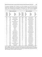
Mechatronic Systems, Simulation, Modeling and Control Part 7 ppt

MechatronicSystems,Simulation,ModellingandControl182

where
 
1
,
K
diag k k
 

and assume that
 
1
0
K
B

 because matrix
0
BK must be positive
definite. Moreover
IBK 
0
assures decoupling of fast mode channels, which makes
controller’s tuning simpler.

The dynamic part of the control law from (26) has the following form:

     
     
 

3 2 1
3 2
,2 ,1 ,0
3 2 1
3 2 2
0
3 3
3 3
d d d
k
         
    
      

        
   
     

(37)
     
     
 
3 2 1
3 2
,2 ,1 ,0
3 2 1
3 2 2
0
3 3
3 3

d d d
k
         
    
      

        
   
     

(38)

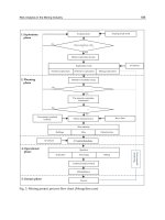
The entire closed loop system is presented in Fig.3.


Fig. 3. Closed-loop system

5. Results of control experiments

In this section, we present the results of experiment which was conducted on the helicopter
model HUMUSOFT CE150, to evaluate the performance of a designed control system.
As the user communicates with the system via Matlab Real Time Toolbox interface, all
input/output signals are scaled into the interval <-1,+1>, where value ”1” is called Machine
Unit and such a signal has no physical dimension. This will be referred in the following text
as MU.
The presented maneuver (experiment 1) consisted in transition with predefined dynamics
from one steady-state angular position to another. Hereby, the control system accomplished
a tracking task of reference signal. The second experiment was chosen to expose
a robustness of the controller under transient and steady-state conditions. During the
experiment, the entire control system was subjected to external disturbances in the form of

a wind gust. Practically this perturbation was realized mechanically by pushing the
helicopter body in required direction with suitable force. The helicopter was disturbed twice
during the test:


1
130 ,t s


2
170 t s .

5.1 Experiment 1 − tracking of a reference trajectory

Fig. 4. Time history of pitch angle




Fig. 5. Time history of yaw angle




Fig. 6. Time history of main motor voltage
1
u


Fig. 7. Time history of tail motor voltage

2
u

ApplicationofHigherOrderDerivativestoHelicopterModelControl 183

where
 
1
,
K
diag k k



and assume that
 
1
0
K
B

 because matrix
0
BK must be positive
definite. Moreover
IBK

0
assures decoupling of fast mode channels, which makes
controller’s tuning simpler.

The dynamic part of the control law from (26) has the following form:

     
     
 
3 2 1
3 2
,2 ,1 ,0
3 2 1
3 2 2
0
3 3
3 3
d d d
k
         
    
      

        
   
     

(37)
     
     
 
3 2 1
3 2

,2 ,1 ,0
3 2 1
3 2 2
0
3 3
3 3
d d d
k
         
    
      

        
   
     

(38)

The entire closed loop system is presented in Fig.3.


Fig. 3. Closed-loop system

5. Results of control experiments

In this section, we present the results of experiment which was conducted on the helicopter
model HUMUSOFT CE150, to evaluate the performance of a designed control system.
As the user communicates with the system via Matlab Real Time Toolbox interface, all
input/output signals are scaled into the interval <-1,+1>, where value ”1” is called Machine
Unit and such a signal has no physical dimension. This will be referred in the following text

as MU.
The presented maneuver (experiment 1) consisted in transition with predefined dynamics
from one steady-state angular position to another. Hereby, the control system accomplished
a tracking task of reference signal. The second experiment was chosen to expose
a robustness of the controller under transient and steady-state conditions. During the
experiment, the entire control system was subjected to external disturbances in the form of
a wind gust. Practically this perturbation was realized mechanically by pushing the
helicopter body in required direction with suitable force. The helicopter was disturbed twice
during the test:


1
130 ,t s


2
170 t s .

5.1 Experiment 1 − tracking of a reference trajectory

Fig. 4. Time history of pitch angle




Fig. 5. Time history of yaw angle


Fig. 6. Time history of main motor voltage
1
u


Fig. 7. Time history of tail motor voltage
2
u

MechatronicSystems,Simulation,ModellingandControl184

5.2 Experiment 2 − influence of a wind gust in vertical plane

Fig. 8. Time history of pitch angle



Fig. 9. Time history of yaw angle



Fig. 10. Time history of main motor voltage
1
u

Fig. 11. Time history of tail motor voltage
2
u

6. Conclusion

The applied method allows to create the expected outputs for multi-input multi-output
nonlinear time-varying physical object, like an exemplary laboratory model of helicopter,
and provides independent desired dynamics in control channels. The peculiarity of the
propose approach is the application of the higher order derivatives jointly with high gain in
the control law. This approach and structure of the control system is the implementation of
the model reference control. The resulting controller is a combination of a low-order linear
dynamical system and a matrix whose entries depend non-linearly on some known process
variables. It becomes that the proposed structure and method is insensitive to external
disturbances and also plant parameter changes, and hereby possess a robustness aspects.
The results suggest that the approach we were concerned with can be applied in some
region of automation, for example in power electronics.

7. Acknowledgements

This work has been granted by the Polish Ministry of Science and Higher Education from
funds for years 2008-2011.

8. References

Astrom, K. J. & Wittenmark, B. (1994). Adaptive control. Addison-Wesley Longman
Publishing Co., Inc. Boston, MA, USA.
Balas, G.; Garrard, W. & Reiner, J. (1995). Robust dynamic inversion for control of highly
maneuverable aircraft, J. of Guidance Control & Dynamics, Vol. 18, No. 1, pp. 18-24.
Błachuta, M.; Yurkevich, V. D. & Wojciechowski, K. (1999). Robust quasi NID aircraft 3D
flight control under sensor noise, Kybernetika, Vol. 35, No.5, pp. 637-650.
Castillo, P.; Lozano, R. & Dzul, A. E. (2005). Modelling and Control of Mini-flying Machines.
Springer-Verlag.
Czyba, R. & Błachuta, M. (2003). Dynamic contraction method approach to robust

longitudinal flight control under aircraft parameters variations, Proceedings of the
AIAA Conference, AIAA 2003-5554, Austin, USA.
Horacek P. (1993). Helicopter Model CE 150 – Educational Manual, Czech Technical
University in Prague.
Isidori, A. & Byrnes, C. I. (1990). Output regulation of nonlinear systems, IEEE Trans.
Automat. Control, Vol. 35, pp. 131-140.
Slotine, J. J. & Li, W. (1991). Applied Nonlinear Control. Prentice Hall, Englewood Cliffs.
Szafrański, G. & Czyba R. (2008). Fast prototyping of three-phase BLDC Motor Controller
designed on the basis of Dynamic Contraction Method, Proceedings of the IEEE
10
th
International Workshop on Variable Structure Systems, pp. 100-105, Turkey.
Utkin, V. I. (1992). Sliding modes in control and optimization. Springer-Verlag.
Valavanis, K. P. (2007). Advances in Unmanned Aerial Vehicles. Springer-Verlag.
Vostrikov, A. S. & Yurkevich, V. D. (1993). Design of control systems by means of
Localisation Method, Preprints of 12-th IFAC World Congress, Vol. 8, pp. 47-50.
Yurkevich, V. D. (2004). Design of Nonlinear Control Systems with the Highest Derivative in
Feedback. World Scientific Publishing.
ApplicationofHigherOrderDerivativestoHelicopterModelControl 185

5.2 Experiment 2 − influence of a wind gust in vertical plane

Fig. 8. Time history of pitch angle



Fig. 9. Time history of yaw angle


Fig. 10. Time history of main motor voltage
1
u

Fig. 11. Time history of tail motor voltage
2
u


6. Conclusion

The applied method allows to create the expected outputs for multi-input multi-output
nonlinear time-varying physical object, like an exemplary laboratory model of helicopter,
and provides independent desired dynamics in control channels. The peculiarity of the
propose approach is the application of the higher order derivatives jointly with high gain in
the control law. This approach and structure of the control system is the implementation of
the model reference control. The resulting controller is a combination of a low-order linear
dynamical system and a matrix whose entries depend non-linearly on some known process
variables. It becomes that the proposed structure and method is insensitive to external
disturbances and also plant parameter changes, and hereby possess a robustness aspects.
The results suggest that the approach we were concerned with can be applied in some
region of automation, for example in power electronics.

7. Acknowledgements

This work has been granted by the Polish Ministry of Science and Higher Education from
funds for years 2008-2011.

8. References

Astrom, K. J. & Wittenmark, B. (1994). Adaptive control. Addison-Wesley Longman
Publishing Co., Inc. Boston, MA, USA.
Balas, G.; Garrard, W. & Reiner, J. (1995). Robust dynamic inversion for control of highly
maneuverable aircraft, J. of Guidance Control & Dynamics, Vol. 18, No. 1, pp. 18-24.
Błachuta, M.; Yurkevich, V. D. & Wojciechowski, K. (1999). Robust quasi NID aircraft 3D
flight control under sensor noise, Kybernetika, Vol. 35, No.5, pp. 637-650.
Castillo, P.; Lozano, R. & Dzul, A. E. (2005). Modelling and Control of Mini-flying Machines.
Springer-Verlag.
Czyba, R. & Błachuta, M. (2003). Dynamic contraction method approach to robust
longitudinal flight control under aircraft parameters variations, Proceedings of the
AIAA Conference, AIAA 2003-5554, Austin, USA.
Horacek P. (1993). Helicopter Model CE 150 – Educational Manual, Czech Technical
University in Prague.
Isidori, A. & Byrnes, C. I. (1990). Output regulation of nonlinear systems, IEEE Trans.
Automat. Control, Vol. 35, pp. 131-140.
Slotine, J. J. & Li, W. (1991). Applied Nonlinear Control. Prentice Hall, Englewood Cliffs.
Szafrański, G. & Czyba R. (2008). Fast prototyping of three-phase BLDC Motor Controller
designed on the basis of Dynamic Contraction Method, Proceedings of the IEEE
10
th
International Workshop on Variable Structure Systems, pp. 100-105, Turkey.
Utkin, V. I. (1992). Sliding modes in control and optimization. Springer-Verlag.
Valavanis, K. P. (2007). Advances in Unmanned Aerial Vehicles. Springer-Verlag.
Vostrikov, A. S. & Yurkevich, V. D. (1993). Design of control systems by means of
Localisation Method, Preprints of 12-th IFAC World Congress, Vol. 8, pp. 47-50.
Yurkevich, V. D. (2004). Design of Nonlinear Control Systems with the Highest Derivative in
Feedback. World Scientific Publishing.
MechatronicSystems,Simulation,ModellingandControl186
LaboratoryExperimentationofGuidanceandControl
ofSpacecraftDuringOn-orbitProximityManeuvers 187

Laboratory Experimentation of Guidance and Control of Spacecraft
DuringOn-orbitProximityManeuvers
JasonS.HallandMarcelloRomano
X

Laboratory Experimentation of Guidance
and Control of Spacecraft During
On-orbit Proximity Maneuvers

Jason S. Hall and Marcello Romano
Naval Postgraduate School
Monterey, CA, USA

1. Introduction

The traditional spacecraft system is a monolithic structure with a single mission focused
design and lengthy production and qualification schedules coupled with enormous cost.
Additionally, there rarely, if ever, is any designed preventive maintenance plan or re-fueling
capability. There has been much research in recent years into alternative options. One
alternative option involves autonomous on-orbit servicing of current or future monolithic
spacecraft systems. The U.S. Department of Defense (DoD) embarked on a highly successful
venture to prove out such a concept with the Defense Advanced Research Projects Agency’s
(DARPA’s) Orbital Express program. Orbital Express demonstrated all of the enabling
technologies required for autonomous on-orbit servicing to include refueling, component
transfer, autonomous satellite grappling and berthing, rendezvous, inspection, proximity
operations, docking and undocking, and autonomous fault recognition and anomaly
handling (Kennedy, 2008). Another potential option involves a paradigm shift from the
monolithic spacecraft system to one involving multiple interacting spacecraft that can
autonomously assemble and reconfigure. Numerous benefits are associated with
autonomous spacecraft assemblies, ranging from a removal of significant intra-modular

reliance that provides for parallel design, fabrication, assembly and validation processes to
the inherent smaller nature of fractionated systems which allows for each module to be
placed into orbit separately on more affordable launch platforms (Mathieu, 2005).
With respect specifically to the validation process, the significantly reduced dimensions and
mass of aggregated spacecraft when compared to the traditional monolithic spacecraft allow
for not only component but even full-scale on-the-ground Hardware-In-the-Loop (HIL)
experimentation. Likewise, much of the HIL experimentation required for on-orbit servicing
of traditional spacecraft systems can also be accomplished in ground-based laboratories
(Creamer, 2007). This type of HIL experimentation complements analytical methods and
numerical simulations by providing a low-risk, relatively low-cost and potentially high-
return method for validating the technology, navigation techniques and control approaches
associated with spacecraft systems. Several approaches exist for the actual HIL testing in a
laboratory environment with respect to spacecraft guidance, navigation and control. One
11
MechatronicSystems,Simulation,ModellingandControl188
such method involves reproduction of the kinematics and vehicle dynamics for 3-DoF (two
horizontal translational degrees and one rotational degree about the vertical axis) through
the use of robotic spacecraft simulators that float via planar air bearings on a flat horizontal
floor. This particular method is currently being employed by several research institutions
and is the validation method of choice for our research into GNC algorithms for proximity
operations at the Naval Postgraduate School (Machida et al., 1992; Ullman, 1993; Corrazzini
& How, 1998; Marchesi et al., 2000; Ledebuhr et al., 2001; Nolet et al., 2005; LeMaster et al.,
2006; Romano et al., 2007). With respect to spacecraft involved in proximity operations, the
in-plane and cross-track dynamics are decoupled, as modeled by the Hill-Clohessy-
Wiltshire (HCW) equations, thus the reduction to 3-Degree of Freedom (DoF) does not
appear to be a critical limiter. One consideration involves the reduction of the vehicle
dynamics to one of a double integrator. However, the orbital dynamics can be considered to
be a disturbance that needs to be compensated for by the spacecraft navigation and control
system during the proximity navigation and assembly phase of multiple systems. Thus the
flat floor testbed can be used to capture many of the critical aspects of an actual autonomous

proximity maneuver that can then be used for validation of numerical simulations. Portions
of the here-in described testbed, combined with the first generation robotic spacecraft
simulator of the Spacecraft Robotics Laboratory (SRL) at Naval Postgraduate School (NPS),
have been employed to propose and experimentally validate control algorithms. The
interested reader is referred to (Romano et al., 2007) for a full description of this robotic
spacecraft simulator and the associated HIL experiments involving its demonstration of
successful autonomous spacecraft approach and docking maneuvers to a collaborative
target with a prototype docking interface of the Orbital Express program.
Given the requirement for spacecraft aggregates to rendezvous and dock during the final
phases of assembly and a desire to maximize the useable surface area of the spacecraft for
power generation, sensor packages, docking mechanisms and payloads while minimizing
thruster impingement, control of such systems using the standard control actuator
configuration of fixed thrusters on each face coupled with momentum exchange devices can
be challenging if not impossible. For such systems, a new and unique configuration is
proposed which may capitalize, for instance, on the recently developed carpal robotic joint
invented by Dr. Steven Canfield with its hemispherical vector space (Canfield, 1998). It is
here demonstrated through Lie algebra analytical methods and experimental results that
two vectorable in-plane thrusters in an opposing configuration can yield a minimum set of
actuators for a controllable system. It will also be shown that by coupling the proposed set
of vectorable thrusters with a single degree of freedom Control Moment Gyroscope, an
additional degree of redundancy can be gained. Experimental results are included using
SRL’s second generation reduced order (3 DoF) spacecraft simulator. A general overview of
this spacecraft simulator is presented in this chapter (additional details on the simulators
can be found in: Hall, 2006; Eikenberry, 2006; Price, W., 2006; Romano & Hall, 2006; Hall &
Romano, 2007a; Hall & Romano, 2007b).
While presenting an overview of a robotic testbed for HIL experimentation of guidance and
control algorithms for on-orbit proximity maneuvers, this chapter specifically focuses on
exploring the feasibility, design and evaluation in a 3-DoF environment of a vectorable
thruster configuration combined with optional miniature single gimbaled control moment
gyro (MSGCMG) for an agile small spacecraft. Specifically, the main aims are to present and

practically confirm the theoretical basis of small-time local controllability for this unique
actuator configuration through both analytical and numerical simulations performed in
previous works (Romano & Hall, 2006; Hall & Romano, 2007a; Hall & Romano, 2007b) and
to validate the viability of using this minimal control actuator configuration on a small
spacecraft in a practical way. Furthermore, the experimental work is used to confirm the
controllability of this configuration along a fully constrained trajectory through the
employment of a smooth feedback controller based on state feedback linearization and
linear quadratic regulator techniques and proper state estimation methods. The chapter is
structured as follows: First the design of the experimental testbed including the floating
surface and the second generation 3-DoF spacecraft simulator is introduced. Then the
dynamics model for the spacecraft simulator with vectorable thrusters and momentum
exchange device are formulated. The controllability concerns associated with this uniquely
configured system are then addressed with a presentation of the minimum number of
control inputs to ensure small time local controllability. Next, a formal development is
presented for the state feedback linearized controller, state estimation methods, Schmitt
trigger and Pulse Width Modulation scheme. Finally, experimental results are presented.

2. The NPS Robotic Spacecraft Simulator Testbed

Three generations of robotic spacecraft simulators have been developed at the NPS
Spacecraft Robotics Laboratory, in order to provide for relatively low-cost HIL
experimentation of GNC algorithms for spacecraft proximity maneuvers (see Fig.1). In
particular, the second generation robotic spacecraft simulator testbed is used for the here-in
presented research. The whole spacecraft simulator testbed consists of three components.
The two components specifically dedicated to HIL experimentation in 3-DoF are a floating
surface with an indoor pseudo-GPS (iGPS) measurement system and one 3-DoF
autonomous spacecraft simulator. The third component of the spacecraft simulator testbed
is a 6-DoF simulator stand-alone computer based spacecraft simulator and is separated from
the HIL components. Additionally, an off-board desktop computer is used to support the 3-
DoF spacecraft simulator by providing the capability to upload software, initiate

experimental testing, receive logged data during testing and process the iGPS position
coordinates. Fig. 2 depicts the robotic spacecraft simulator in the Proximity Operations
Simulator Facility (POSF) at NPS with key components identified. The main testbed systems
are briefly described in the next sections with further details given in (Hall, 2006; Price, 2006;
Eikenberry, 2006; Romano & Hall, 2006; Hall & Romano, 2007a; Hall & Romano 2007b).

LaboratoryExperimentationofGuidanceandControl
ofSpacecraftDuringOn-orbitProximityManeuvers 189
such method involves reproduction of the kinematics and vehicle dynamics for 3-DoF (two
horizontal translational degrees and one rotational degree about the vertical axis) through
the use of robotic spacecraft simulators that float via planar air bearings on a flat horizontal
floor. This particular method is currently being employed by several research institutions
and is the validation method of choice for our research into GNC algorithms for proximity
operations at the Naval Postgraduate School (Machida et al., 1992; Ullman, 1993; Corrazzini
& How, 1998; Marchesi et al., 2000; Ledebuhr et al., 2001; Nolet et al., 2005; LeMaster et al.,
2006; Romano et al., 2007). With respect to spacecraft involved in proximity operations, the
in-plane and cross-track dynamics are decoupled, as modeled by the Hill-Clohessy-
Wiltshire (HCW) equations, thus the reduction to 3-Degree of Freedom (DoF) does not
appear to be a critical limiter. One consideration involves the reduction of the vehicle
dynamics to one of a double integrator. However, the orbital dynamics can be considered to
be a disturbance that needs to be compensated for by the spacecraft navigation and control
system during the proximity navigation and assembly phase of multiple systems. Thus the
flat floor testbed can be used to capture many of the critical aspects of an actual autonomous
proximity maneuver that can then be used for validation of numerical simulations. Portions
of the here-in described testbed, combined with the first generation robotic spacecraft
simulator of the Spacecraft Robotics Laboratory (SRL) at Naval Postgraduate School (NPS),
have been employed to propose and experimentally validate control algorithms. The
interested reader is referred to (Romano et al., 2007) for a full description of this robotic
spacecraft simulator and the associated HIL experiments involving its demonstration of
successful autonomous spacecraft approach and docking maneuvers to a collaborative

target with a prototype docking interface of the Orbital Express program.
Given the requirement for spacecraft aggregates to rendezvous and dock during the final
phases of assembly and a desire to maximize the useable surface area of the spacecraft for
power generation, sensor packages, docking mechanisms and payloads while minimizing
thruster impingement, control of such systems using the standard control actuator
configuration of fixed thrusters on each face coupled with momentum exchange devices can
be challenging if not impossible. For such systems, a new and unique configuration is
proposed which may capitalize, for instance, on the recently developed carpal robotic joint
invented by Dr. Steven Canfield with its hemispherical vector space (Canfield, 1998). It is
here demonstrated through Lie algebra analytical methods and experimental results that
two vectorable in-plane thrusters in an opposing configuration can yield a minimum set of
actuators for a controllable system. It will also be shown that by coupling the proposed set
of vectorable thrusters with a single degree of freedom Control Moment Gyroscope, an
additional degree of redundancy can be gained. Experimental results are included using
SRL’s second generation reduced order (3 DoF) spacecraft simulator. A general overview of
this spacecraft simulator is presented in this chapter (additional details on the simulators
can be found in: Hall, 2006; Eikenberry, 2006; Price, W., 2006; Romano & Hall, 2006; Hall &
Romano, 2007a; Hall & Romano, 2007b).
While presenting an overview of a robotic testbed for HIL experimentation of guidance and
control algorithms for on-orbit proximity maneuvers, this chapter specifically focuses on
exploring the feasibility, design and evaluation in a 3-DoF environment of a vectorable
thruster configuration combined with optional miniature single gimbaled control moment
gyro (MSGCMG) for an agile small spacecraft. Specifically, the main aims are to present and
practically confirm the theoretical basis of small-time local controllability for this unique
actuator configuration through both analytical and numerical simulations performed in
previous works (Romano & Hall, 2006; Hall & Romano, 2007a; Hall & Romano, 2007b) and
to validate the viability of using this minimal control actuator configuration on a small
spacecraft in a practical way. Furthermore, the experimental work is used to confirm the
controllability of this configuration along a fully constrained trajectory through the
employment of a smooth feedback controller based on state feedback linearization and

linear quadratic regulator techniques and proper state estimation methods. The chapter is
structured as follows: First the design of the experimental testbed including the floating
surface and the second generation 3-DoF spacecraft simulator is introduced. Then the
dynamics model for the spacecraft simulator with vectorable thrusters and momentum
exchange device are formulated. The controllability concerns associated with this uniquely
configured system are then addressed with a presentation of the minimum number of
control inputs to ensure small time local controllability. Next, a formal development is
presented for the state feedback linearized controller, state estimation methods, Schmitt
trigger and Pulse Width Modulation scheme. Finally, experimental results are presented.

2. The NPS Robotic Spacecraft Simulator Testbed

Three generations of robotic spacecraft simulators have been developed at the NPS
Spacecraft Robotics Laboratory, in order to provide for relatively low-cost HIL
experimentation of GNC algorithms for spacecraft proximity maneuvers (see Fig.1). In
particular, the second generation robotic spacecraft simulator testbed is used for the here-in
presented research. The whole spacecraft simulator testbed consists of three components.
The two components specifically dedicated to HIL experimentation in 3-DoF are a floating
surface with an indoor pseudo-GPS (iGPS) measurement system and one 3-DoF
autonomous spacecraft simulator. The third component of the spacecraft simulator testbed
is a 6-DoF simulator stand-alone computer based spacecraft simulator and is separated from
the HIL components. Additionally, an off-board desktop computer is used to support the 3-
DoF spacecraft simulator by providing the capability to upload software, initiate
experimental testing, receive logged data during testing and process the iGPS position
coordinates. Fig. 2 depicts the robotic spacecraft simulator in the Proximity Operations
Simulator Facility (POSF) at NPS with key components identified. The main testbed systems
are briefly described in the next sections with further details given in (Hall, 2006; Price, 2006;
Eikenberry, 2006; Romano & Hall, 2006; Hall & Romano, 2007a; Hall & Romano 2007b).

MechatronicSystems,Simulation,ModellingandControl190

Fig. 1. Three generations of spacecraft simulator at the NPS Spacecraft Robotics Laboratory
(first, second and third generations from left to right)

2.1 Floating Surface
A 4.9 m by 4.3 m epoxy floor surface provides the base for the floatation of the spacecraft
simulator. The use of planar air bearings on the simulator reduces the friction to a negligible
level and with an average residual slope angle of approximately 2.6x10
-3
deg for the floating
surface, the average residual acceleration due to gravity is approximately 1.8x10
-3
ms
-2
. This
value of acceleration is 2 orders of magnitude lower than the nominal amplitude of the
measured acceleration differences found during reduced gravity phases of parabolic flights
(Romano et al, 2007).

Fig. 2. SRL's 2nd Generation 3-DoF Spacecraft Simulator

2.2 3-DoF Robotic Spacecraft Simulator
SRL’s second generation robotic spacecraft simulator is modularly constructed with three
easily assembled sections dedicated to each primary subsystem. Prefabricated 6105-T5
Aluminum fractional t-slotted extrusions form the cage of the vehicle while one square foot,
.25 inch thick static dissipative rigid plastic sheets provide the upper and lower decks of
each module. The use of these materials for the basic structural requirements provides a
high strength to weight ratio and enable rapid assembly and reconfiguration. Table 1 reports
the key parameters of the 3-DoF spacecraft simulator.

2.2.1 Propulsion and Flotation Subsystems
The lowest module houses the flotation and propulsion subsystems. The flotation subsystem
is composed of four planar air bearings, an air filter assembly, dual 4500 PSI (31.03 MPa)
carbon-fiber spun air cylinders and a dual manifold pressure reducer to provide 75 PSI (.51
MPa). This pressure with a volume flow rate for each air bearing of 3.33 slfm (3.33 x 10
-3

m
3
/min) is sufficient to keep the simulator in a friction-free state for nearly 40 minutes of
continuous experimentation time. The propulsion subsystem is composed of dual vectorable
supersonic on-off cold-gas thrusters and a separate dual carbon-fiber spun air cylinder and
pressure reducer package regulated at 60 PSI (.41 MPa) and has the capability of providing
the system 31.1 m/s

V .

2.2.2 Electronic and Power Distribution Subsystems
The power distribution subsystem is composed of dual lithium-ion batteries wired in
parallel to provide 28 volts for up to 12 Amp-Hours and is housed in the second deck of the
simulator. A four port DC-DC converter distributes the requisite power for the system at 5,
12 or 24 volts DC. An attached cold plate provides heat transfer from the array to the power
system mounting deck in the upper module. The current power requirements include a
single PC-104 CPU stack, a wireless router, three motor controllers, three separate normally-
closed solenoid valves for thruster and air bearing actuation, a fiber optic gyro, a
magnetometer and a wireless server for transmission of the vehicle’s position via the
pseudo-GPS system.

LaboratoryExperimentationofGuidanceandControl
ofSpacecraftDuringOn-orbitProximityManeuvers 191

Fig. 1. Three generations of spacecraft simulator at the NPS Spacecraft Robotics Laboratory
(first, second and third generations from left to right)

2.1 Floating Surface
A 4.9 m by 4.3 m epoxy floor surface provides the base for the floatation of the spacecraft
simulator. The use of planar air bearings on the simulator reduces the friction to a negligible
level and with an average residual slope angle of approximately 2.6x10
-3
deg for the floating
surface, the average residual acceleration due to gravity is approximately 1.8x10
-3
ms
-2
. This
value of acceleration is 2 orders of magnitude lower than the nominal amplitude of the

measured acceleration differences found during reduced gravity phases of parabolic flights
(Romano et al, 2007).

Fig. 2. SRL's 2nd Generation 3-DoF Spacecraft Simulator

2.2 3-DoF Robotic Spacecraft Simulator
SRL’s second generation robotic spacecraft simulator is modularly constructed with three
easily assembled sections dedicated to each primary subsystem. Prefabricated 6105-T5
Aluminum fractional t-slotted extrusions form the cage of the vehicle while one square foot,
.25 inch thick static dissipative rigid plastic sheets provide the upper and lower decks of
each module. The use of these materials for the basic structural requirements provides a
high strength to weight ratio and enable rapid assembly and reconfiguration. Table 1 reports
the key parameters of the 3-DoF spacecraft simulator.

2.2.1 Propulsion and Flotation Subsystems
The lowest module houses the flotation and propulsion subsystems. The flotation subsystem
is composed of four planar air bearings, an air filter assembly, dual 4500 PSI (31.03 MPa)
carbon-fiber spun air cylinders and a dual manifold pressure reducer to provide 75 PSI (.51
MPa). This pressure with a volume flow rate for each air bearing of 3.33 slfm (3.33 x 10
-3

m
3
/min) is sufficient to keep the simulator in a friction-free state for nearly 40 minutes of
continuous experimentation time. The propulsion subsystem is composed of dual vectorable
supersonic on-off cold-gas thrusters and a separate dual carbon-fiber spun air cylinder and
pressure reducer package regulated at 60 PSI (.41 MPa) and has the capability of providing
the system 31.1 m/s V .

2.2.2 Electronic and Power Distribution Subsystems

The power distribution subsystem is composed of dual lithium-ion batteries wired in
parallel to provide 28 volts for up to 12 Amp-Hours and is housed in the second deck of the
simulator. A four port DC-DC converter distributes the requisite power for the system at 5,
12 or 24 volts DC. An attached cold plate provides heat transfer from the array to the power
system mounting deck in the upper module. The current power requirements include a
single PC-104 CPU stack, a wireless router, three motor controllers, three separate normally-
closed solenoid valves for thruster and air bearing actuation, a fiber optic gyro, a
magnetometer and a wireless server for transmission of the vehicle’s position via the
pseudo-GPS system.















MechatronicSystems,Simulation,ModellingandControl192
Subsystem Characteristic
Parameter
Structure Length and width
.30 m
Height

.69 m
Mass (Overall)
26 kg

z
J
(Overall)
.40 kg-m
2
Propulsion Propellant
Compressed Air
Equiv. storage capacity
.05 m
3
@ 31.03 Mpa
Operating pressure
.41 Mpa
Thrust (x2)
.159 N
ISP
34.3 s

Total
V
31.1 m/s
Flotation Propellant
Air
Equiv. storage capacity
0.05 m
3

@ 31.03 Mpa
Operating pressure
.51 Mpa
Linear air bearing (x4)
32 mm diameter
Continuous operation
~40 min
CMG Attitude Control Max torque
.668 Nm
Momentum storage
.098 Nms
Electrical & Electronic Battery type
Lithium-Ion
Storage capacity
12 Ah @ 28V
Continuous Operation
~6 h
Computer
1 PC104 Pentium III
Sensors Fiber optic gyro
KVH Model DSP-3000
Position sensor
Metris iGPS
Magnetometer
MicroStrain 3DM-GX1
Table 1. Key Parameters of the 2nd generation 3-DoF Robotic Spacecraft Simulator

2.2.3 Translation and Attitude Control System Actuators
The 3-DoF robotic spacecraft simulator includes actuators to provide both translational
control and attitude control. A full development of the controllability for this unique

configuration of dual rotating thrusters and one-axis Miniature-Single Gimbaled Control
Moment Gyro (MSGCMG) will be demonstrated in subsequent sections of this paper. The
translational control is provided by two cold-gas on-off supersonic nozzle thrusters in a
dual vectorable configuration. Each thruster is limited in a region

 2
with respect to the
face normal and, through experimental testing at the supplied pressure, has been
demonstrated to have an ISP of 34.3 s and able to provide .159 N of thrust with less than 10
msec actuation time (Lugini, 2008). The MSGCMG is capable of providing .668 Nm of torque
with a maximum angular momentum of .098 Nms.

2.3 6-DoF Computer-Based Numerical Spacecraft Simulator
A separate component of SRL’s spacecraft simulator testbed at NPS is a 6-DoF computer-
based spacecraft simulator. This simulator enables full 6-DoF numerical simulations to be
conducted with realistic orbital perturbations including aerodynamic, solar pressure and
third-body effects, and earth oblateness up to J4. Similar to the 3-DoF robotic simulator, the
numerical simulator is also modularly designed within a MATLAB®/Simulink®
architecture to allow near seamless integration and testing of developed guidance and
control algorithms. Additionally, by using the MATLAB®/Simulink® architecture with the
added Real Time Workshop™ toolbox, the developed control algorithms can be readily
transitioned into C-code for direct deployment onto the 3-DoF robotic simulator’s onboard
processor. A full discussion of the process by which this is accomplished and simplified for
rapid real-time experimentation on the 3-DoF testbed for either the proprietary MATLAB®
based XPCTarget™ operating system is given in (Hall, 2006; Price, 2006) or for an open-
source Linux based operating system with the Real Time Application Interface (RTAI) is
given in (Bevilacqua et al., 2009).

3. Dynamics of a 3-DoF Spacecraft Simulator with Vectorable Thrusters and
Momentum Exchange Device

Two sets of coordinate frame are established for reference: the inertial coordinate system
(ICS) designated by XYZ and body-fixed coordinate system (BCS) designated by xyz. These
reference frames are depicted in Fig. 3 along with the necessary external forces and
parameters required to properly define the simulators motion. The origin of the body-fixed
coordinate system is taken to be the center of mass C of the spacecraft simulator and this is
assumed to be collocated with the simulator’s geometric center. The body z-axis is aligned
with the inertial Z-axis while the body x-axis is in line with the thrusters points of action. In
the ICS, the position and velocity vectors of C are given by
X and V so that


,X YX marks
the position of the simulator with respect to the origin of the ICS as measured by the inertial
measurement sensors and provides the vehicle’s two degrees of translational freedom. The
vehicle’s rotational freedom is described by an angle of rotation

between the x-axis and
the X-axis about the z-axis. The angular velocity is thus limited to one degree of freedom
and is denoted by

z
. The spacecraft simulator is assumed to be rigid and therefore a
constant moment of inertia (
z
J
) exists about the z-axis. Furthermore, any changes to the
mass of the simulator (
m
) due to thruster firing are neglected.

The forces imparted at a distance L from the center of mass by the vectorable on-off
thrusters are denoted by
1 2

and F F
respectively. The direction of the thrust vector
1
F
is
determined by

1
which is the angle measured from the outward normal of face one in a
clockwise direction (right-hand rotation) to where thruster one’s nozzle is pointing.
Likewise, the direction of the thrust vector
2
F

is determined by

2
which is the angle
measured from the outward normal of face two in a clockwise direction (right-hand
rotation) to where thruster two’s nozzle is pointing. The torque imparted on the vehicle by a
momentum exchange device such as a control moment gyro is denoted by
M
ED
T
and can be
constrained to exist only about the yaw axis as demonstrated in (Hall, 2006; Romano & Hall,

2006).

LaboratoryExperimentationofGuidanceandControl
ofSpacecraftDuringOn-orbitProximityManeuvers 193
Subsystem Characteristic
Parameter
Structure Length and width
.30 m
Height
.69 m
Mass (Overall)
26 kg

z
J
(Overall)
.40 kg-m
2
Propulsion Propellant
Compressed Air
Equiv. storage capacity
.05 m
3
@ 31.03 Mpa
Operating pressure
.41 Mpa
Thrust (x2)
.159 N
ISP
34.3 s

Total

V
31.1 m/s
Flotation Propellant
Air
Equiv. storage capacity
0.05 m
3
@ 31.03 Mpa
Operating pressure
.51 Mpa
Linear air bearing (x4)
32 mm diameter
Continuous operation
~40 min
CMG Attitude Control Max torque
.668 Nm
Momentum storage
.098 Nms
Electrical & Electronic Battery type
Lithium-Ion
Storage capacity
12 Ah @ 28V
Continuous Operation
~6 h
Computer
1 PC104 Pentium III
Sensors Fiber optic gyro

KVH Model DSP-3000
Position sensor
Metris iGPS
Magnetometer
MicroStrain 3DM-GX1
Table 1. Key Parameters of the 2nd generation 3-DoF Robotic Spacecraft Simulator

2.2.3 Translation and Attitude Control System Actuators
The 3-DoF robotic spacecraft simulator includes actuators to provide both translational
control and attitude control. A full development of the controllability for this unique
configuration of dual rotating thrusters and one-axis Miniature-Single Gimbaled Control
Moment Gyro (MSGCMG) will be demonstrated in subsequent sections of this paper. The
translational control is provided by two cold-gas on-off supersonic nozzle thrusters in a
dual vectorable configuration. Each thruster is limited in a region

 2
with respect to the
face normal and, through experimental testing at the supplied pressure, has been
demonstrated to have an ISP of 34.3 s and able to provide .159 N of thrust with less than 10
msec actuation time (Lugini, 2008). The MSGCMG is capable of providing .668 Nm of torque
with a maximum angular momentum of .098 Nms.

2.3 6-DoF Computer-Based Numerical Spacecraft Simulator
A separate component of SRL’s spacecraft simulator testbed at NPS is a 6-DoF computer-
based spacecraft simulator. This simulator enables full 6-DoF numerical simulations to be
conducted with realistic orbital perturbations including aerodynamic, solar pressure and
third-body effects, and earth oblateness up to J4. Similar to the 3-DoF robotic simulator, the
numerical simulator is also modularly designed within a MATLAB®/Simulink®
architecture to allow near seamless integration and testing of developed guidance and
control algorithms. Additionally, by using the MATLAB®/Simulink® architecture with the

added Real Time Workshop™ toolbox, the developed control algorithms can be readily
transitioned into C-code for direct deployment onto the 3-DoF robotic simulator’s onboard
processor. A full discussion of the process by which this is accomplished and simplified for
rapid real-time experimentation on the 3-DoF testbed for either the proprietary MATLAB®
based XPCTarget™ operating system is given in (Hall, 2006; Price, 2006) or for an open-
source Linux based operating system with the Real Time Application Interface (RTAI) is
given in (Bevilacqua et al., 2009).

3. Dynamics of a 3-DoF Spacecraft Simulator with Vectorable Thrusters and
Momentum Exchange Device

Two sets of coordinate frame are established for reference: the inertial coordinate system
(ICS) designated by XYZ and body-fixed coordinate system (BCS) designated by xyz. These
reference frames are depicted in Fig. 3 along with the necessary external forces and
parameters required to properly define the simulators motion. The origin of the body-fixed
coordinate system is taken to be the center of mass C of the spacecraft simulator and this is
assumed to be collocated with the simulator’s geometric center. The body z-axis is aligned
with the inertial Z-axis while the body x-axis is in line with the thrusters points of action. In
the ICS, the position and velocity vectors of C are given by
X and V so that


,X YX marks
the position of the simulator with respect to the origin of the ICS as measured by the inertial
measurement sensors and provides the vehicle’s two degrees of translational freedom. The
vehicle’s rotational freedom is described by an angle of rotation

between the x-axis and
the X-axis about the z-axis. The angular velocity is thus limited to one degree of freedom
and is denoted by


z
. The spacecraft simulator is assumed to be rigid and therefore a
constant moment of inertia (
z
J
) exists about the z-axis. Furthermore, any changes to the
mass of the simulator (
m
) due to thruster firing are neglected.
The forces imparted at a distance L from the center of mass by the vectorable on-off
thrusters are denoted by
1 2

and F F
respectively. The direction of the thrust vector
1
F
is
determined by

1
which is the angle measured from the outward normal of face one in a
clockwise direction (right-hand rotation) to where thruster one’s nozzle is pointing.
Likewise, the direction of the thrust vector
2
F

is determined by


2
which is the angle
measured from the outward normal of face two in a clockwise direction (right-hand
rotation) to where thruster two’s nozzle is pointing. The torque imparted on the vehicle by a
momentum exchange device such as a control moment gyro is denoted by
M
ED
T
and can be
constrained to exist only about the yaw axis as demonstrated in (Hall, 2006; Romano & Hall,
2006).

MechatronicSystems,Simulation,ModellingandControl194

Fig. 3. SRL‘s 2nd Generation Spacecraft Simulator Schematic

The translation and attitude motion of the simulator are governed by the equations


 

 












1
1
I B
B
z
B
z z
m
J T
X V
V R F
(1)

where

2B
F
are the thruster inputs limited to the region

 2
with respect to each face
normal and

B
T
is the attitude input.




I
B
R
,
B
F
and
B
T
are given by


 



 

 

 
 
c s
s c
I
B
R
(2)

 
   
      
1 2 1 1 2 2 1 1 2 2
c c , s s
T
B T B T B T
F F F FF F F
(3)



 
     
 
1 1 2 2
s s
B
MED
T T L F F
(4)
where
 


s sin , c cos     
.
The internal dynamics of the vectorable thrusters are assumed to be linear according to the
following equations

     
 
   
 
 
1 1
1 1 1 1 1 2 2 2 2 2
, , ,J T J T
(5)
where
1
J
and
2
J
represent the moments of inertia about each thruster rotational axis
respectively and


1
T
,


2
T
represent the corresponding thruster rotation control input.
The system’s state equation given by Eq. (1) can be rewritten in control-affine system form
as (LaValle, 2006)

//X
x


2
F




2
//Y


M
ED
T

L

1

C

L

1

2

1
F

Y
X

X

y


       

    



1
,
u
x
N
N
i i
i
u G xx f x g x f x x u (6)
where
u

N
is the number of controls. With 
x
N
representing a smooth
x
N
-dimensional
manifold defined be the size of the state-vector and the control vector to be in

u
N
.
Defining
the state vector

10
x
as




1 2 10
, , ,
T
x x xx


    

1 2 1 2
[ , , , , , , , , , ]
x y z
X Y V V and the
control vector

5
u U
as




1 2 5
, , ,
T
u u uu
1 2 1 2
[ , , , , ]
MED
F F T T T
, the system’s state equation,
becomes

   
 
 


   






5 5
6 7 8 9 10 1 5
1
, , , , ,
T
x
x
G x x x x x
G
0
x f x x u 0 u
x
(7)
where the matrix


1
G x is obtained from Eq. (1) as


   
   
 
 
  





  


  





 








1 1
3 4 3 4 3 5 3 5
1 1
3 4 3 4 3 5 3 5
1 1 1
1
4 5
1

2
1
2
c c s s c c s s 0 0 0
c s s c c s s c 0 0 0
( )
s s 0 0
0 0 0 0
0 0 0 0
z z z
m x x x x m x x x x
m x x x x m x x x x
G
J x L J x L J
J
J
x
(8)

With the system in the form of Eq. (6) given the vector fields in Eqs. (7) and (8), and given
that
( )f x
(the drift term) and
( )G x
(the control matrix of control vector fields) are smooth
functions, it is important to note that it is not necessarily possible to obtain zero velocity due
to the influence of the drift term. This fact places the system in the unique subset of control-
affine systems with drift and, as seen later, will call for an additional requirement for
determining the controllability of the system. Furthermore, when studying controllability of
systems, the literature to date restricts the consideration to cases where the control is proper.

Having a proper control implies that the affine hull of the control space is equal to

u
N
or
that the smallest subspace of
U is equal to the number of control vectors and that it is
closed (Sussman, 1987; Sussman, 1990; Bullo & Lewis, 2005; LaValle, 2006). With a system
such as a spacecraft in general or the simplified model of the 3-DoF simulator in particular,
the use of on-off cold-gas thrusters restrict the control space to only positive space with
respect to both thrust vectors leading to an unclosed set and thus improper control space. In
order to overcome this issue, a method which leverages the symmetry of the system is used
by which the controllability of the system is studied by considering only one virtual rotating
thruster that is positioned a distance L from the center of mass with the vectored thrust
resolved into a y and x-component. In considering this system perspective, the thruster
combination now spans

2
and therefore is proper and is analogous to the planar body with
variable-direction force vector considered in (Lewis & Murray, 1997; Bullo & Lewis, 2005).
Furthermore, under the assumption that the control bandwidth of the thrusters’s rotation is
much larger than the control bandwidth of the system dynamics, the internal dynamics of
the vectorable thrusters can be decoupled from the state and control vectors for the system
yielding a thrust vector dependent on simply a commanded angle. Thus the system’s state
vector, assuming that both thrusters and a momentum exchange device are available,
LaboratoryExperimentationofGuidanceandControl
ofSpacecraftDuringOn-orbitProximityManeuvers 195

Fig. 3. SRL‘s 2nd Generation Spacecraft Simulator Schematic

The translation and attitude motion of the simulator are governed by the equations


 

 











1
1
I B
B
z
B
z z
m
J T
X V
V R F
(1)

where

2B
F
are the thruster inputs limited to the region

 2
with respect to each face
normal and

B
T
is the attitude input.



I
B
R
,
B
F
and
B
T
are given by


 














c s
s c
I
B
R
(2)

 
   
      
1 2 1 1 2 2 1 1 2 2
c c , s s
T
B T B T B T
F F F FF F F
(3)




 

    


1 1 2 2
s s
B
MED
T T L F F
(4)
where
 


s sin , c cos     
.
The internal dynamics of the vectorable thrusters are assumed to be linear according to the
following equations

     
 
   
 
 
1 1
1 1 1 1 1 2 2 2 2 2
, , ,J T J T
(5)

where
1
J
and
2
J
represent the moments of inertia about each thruster rotational axis
respectively and


1
T
,


2
T
represent the corresponding thruster rotation control input.
The system’s state equation given by Eq. (1) can be rewritten in control-affine system form
as (LaValle, 2006)

//X
x


2
F




2
//Y


M
ED
T

L

1

C

L

1

2


1
F

Y
X

X

y


       

    



1
,
u
x
N
N
i i
i
u G xx f x g x f x x u (6)
where
u
N
is the number of controls. With 
x
N
representing a smooth
x
N
-dimensional
manifold defined be the size of the state-vector and the control vector to be in


u
N
.
Defining
the state vector

10
x
as


 
1 2 10
, , ,
T
x x xx


    
1 2 1 2
[ , , , , , , , , , ]
x y z
X Y V V and the
control vector

5
u U
as



 
1 2 5
, , ,
T
u u uu
1 2 1 2
[ , , , , ]
MED
F F T T T
, the system’s state equation,
becomes

   
 
 
 
   
 
 

5 5
6 7 8 9 10 1 5
1
, , , , ,
T
x
x
G x x x x x
G
0

x f x x u 0 u
x
(7)
where the matrix


1
G x is obtained from Eq. (1) as


   
   
 
 
  


 
  
 
  
 
 

 
 
 
 
 
1 1

3 4 3 4 3 5 3 5
1 1
3 4 3 4 3 5 3 5
1 1 1
1
4 5
1
2
1
2
c c s s c c s s 0 0 0
c s s c c s s c 0 0 0
( )
s s 0 0
0 0 0 0
0 0 0 0
z z z
m x x x x m x x x x
m x x x x m x x x x
G
J x L J x L J
J
J
x
(8)

With the system in the form of Eq. (6) given the vector fields in Eqs. (7) and (8), and given
that
( )f x
(the drift term) and

( )G x
(the control matrix of control vector fields) are smooth
functions, it is important to note that it is not necessarily possible to obtain zero velocity due
to the influence of the drift term. This fact places the system in the unique subset of control-
affine systems with drift and, as seen later, will call for an additional requirement for
determining the controllability of the system. Furthermore, when studying controllability of
systems, the literature to date restricts the consideration to cases where the control is proper.
Having a proper control implies that the affine hull of the control space is equal to

u
N
or
that the smallest subspace of
U is equal to the number of control vectors and that it is
closed (Sussman, 1987; Sussman, 1990; Bullo & Lewis, 2005; LaValle, 2006). With a system
such as a spacecraft in general or the simplified model of the 3-DoF simulator in particular,
the use of on-off cold-gas thrusters restrict the control space to only positive space with
respect to both thrust vectors leading to an unclosed set and thus improper control space. In
order to overcome this issue, a method which leverages the symmetry of the system is used
by which the controllability of the system is studied by considering only one virtual rotating
thruster that is positioned a distance L from the center of mass with the vectored thrust
resolved into a y and x-component. In considering this system perspective, the thruster
combination now spans

2
and therefore is proper and is analogous to the planar body with
variable-direction force vector considered in (Lewis & Murray, 1997; Bullo & Lewis, 2005).
Furthermore, under the assumption that the control bandwidth of the thrusters’s rotation is
much larger than the control bandwidth of the system dynamics, the internal dynamics of
the vectorable thrusters can be decoupled from the state and control vectors for the system

yielding a thrust vector dependent on simply a commanded angle. Thus the system’s state
vector, assuming that both thrusters and a momentum exchange device are available,
MechatronicSystems,Simulation,ModellingandControl196
becomes


 
  
6
1 2 6
, , , [ , , , , , ]
T
X Y z
x x x X Y V Vx
and the control vector is


  
3
1 2 3
, , [ , , ]
T B B B
x y z
u u u F F Tu U

so that the system’s state equation becomes


   
 

 
 
   
 
 

3 3
4 5 6
1
, , ,0,0,0
T
x
G x x x
G
0
x f x x u u
x
(9)

where the matrix


1
G x
can be obtained by considering the relation of the desired control
vector to the body centered reference system, in the two cases of positive force needed in the
x direction (


B

U
x
 0
) and negative force needed in the x direction (


B
U
x
 0
). In this manner,
the variables in Eq. (8) and Eq. (9) can be defined as




 

   

 

  



 

 


 


1 4 1 4
2
2 5 2 5
1
[ , , ] c , s ,
0
, 0
[ , , ] c , s ,
0
, 0
T B B B
x
y
z MED
B
x
T B B B
x y z MED
B
x
F F T F x F x T
U
d L F
F F T F x F x T
U
d L F
u

u
(10)

yielding the matrix in


1
G x
through substitution into Eq. (8) as


 
 
 
 

 

 
 

 
1 1
3 3
1 1
1 3 3
1 1
c s 0
( ) s c 0
0

z z
m x m x
G m x m x
dJ J
x
(11)

When the desired control input to the system along the body x-axis is zero, both thrusters
can be used to provide a control force along the y-axis, while a momentum exchange device
provides any required torque. In this case, the control vector in (9) becomes


  
2
1 2
, [ , ]
T B B
y z
u u F Tu U
such that the variables in Eq. (8) and (9) can be defined as




 




 


 

      


1 2 4 5
[ , ] ,
0
,
2
T B B
y z MED
B
x
B
y
F T Fs T
U
F F F x x si
g
n U
u
(12)

which yields the matrix


1
G x

through substitution into Eq. (8) as





 

 

 
 
 
1
3
1
1 3
1
2 s 0
( ) 2 c 0
0
z
m x
G m x
J
x
(13)

As will be demonstrated in later, the momentum exchange device is not necessary to ensure
small time controllability for this system. In considering this situation, which also occurs

when a control moment gyroscope is present but is near the singular conditions and
therefore requires desaturation, the thruster not being used for translation control can be
slewed to

 2
depending on the required torque compensation and fired to affect the
desired angular rate change. The desired control input to the system with respect to the
body x-axis
 
B
x
U
can again be used to define the desired variables such that




 



   

 

   



  


 

  


1 4 1 4 2 5
5
2 5 2 5 1 4
4
[ , , ] c , s , s
0
,
2
[ , , ] c , s , s
0
,
2
T B B B
x y z
B
x
T B B B
x y z
B
x
F F T F x F x F d x
U
d L x
F F T F x F x F d x

U
d L x
u
u
(14)

which yields the matrix


1
G x
through substitution into Eq. (8)as


 
 

 

 
 


 













1
1 1
3 3 3
1
1 1
1 3 3 3
1 1
c s s
( ) s c c
0
z z
m x m x md x
G m x m x md x
dJ J
x
(15)

In case of zero force requested along x with only thrusters acting, the system cannot in
general provide the requested torque value.
A key design consideration with this type of control actuator configuration is that with only
the use of an on/off rotating thruster to provide the necessary torque compensation, fine
pointing can be difficult and more fuel is required to affect a desired maneuver involving
both translation and rotation.

4. Small-Time Local Controllability

Before studying the controllability for a nonlinear control-affine system of the form in
Eq. (6), it is important to review several definitions. First, the set of states reachable in time
at most T is given by




0
,R Tx
by solutions of the nonlinear control-affine system.
Definition 1 (Accessibility)
A system is accessible from
0
x
(the initial state) if there exists  0T such that the interior of
 


0
,R tx
is not an empty set for


 0,t T
(Bullo & Lewis, 2005).

Definition 2 (Proper Small Time Local Controllability)
A system is small time locally controllable (STLC) from

0
x
if there exists  0T such that
0
x
lies in the interior of




0
,R tx
for each


 0,t T
for every proper control set U (Bullo &
LaboratoryExperimentationofGuidanceandControl
ofSpacecraftDuringOn-orbitProximityManeuvers 197
becomes


 
  
6
1 2 6
, , , [ , , , , , ]
T
X Y z
x x x X Y V Vx

and the control vector is


  
3
1 2 3
, , [ , , ]
T B B B
x y z
u u u F F Tu U

so that the system’s state equation becomes


   
 
 


   





3 3
4 5 6
1
, , ,0,0,0
T

x
G x x x
G
0
x f x x u u
x
(9)

where the matrix


1
G x
can be obtained by considering the relation of the desired control
vector to the body centered reference system, in the two cases of positive force needed in the
x direction (


B
U
x
 0
) and negative force needed in the x direction (


B
U
x
 0
). In this manner,

the variables in Eq. (8) and Eq. (9) can be defined as




 

   

 

  



 

 

 


1 4 1 4
2
2 5 2 5
1
[ , , ] c , s ,
0
, 0
[ , , ] c , s ,

0
, 0
T B B B
x
y
z MED
B
x
T B B B
x y z MED
B
x
F F T F x F x T
U
d L F
F F T F x F x T
U
d L F
u
u
(10)

yielding the matrix in


1
G x
through substitution into Eq. (8) as

 
 
 













1 1
3 3
1 1
1 3 3
1 1
c s 0
( ) s c 0
0
z z
m x m x
G m x m x
dJ J
x
(11)

When the desired control input to the system along the body x-axis is zero, both thrusters
can be used to provide a control force along the y-axis, while a momentum exchange device
provides any required torque. In this case, the control vector in (9) becomes


  
2
1 2
, [ , ]
T B B
y z
u u F Tu U
such that the variables in Eq. (8) and (9) can be defined as




 




 

 

      



1 2 4 5
[ , ] ,
0
,
2
T B B
y z MED
B
x
B
y
F T Fs T
U
F F F x x si
g
n U
u
(12)

which yields the matrix


1
G x
through substitution into Eq. (8) as


















1
3
1
1 3
1
2 s 0
( ) 2 c 0
0
z
m x
G m x
J
x
(13)

As will be demonstrated in later, the momentum exchange device is not necessary to ensure
small time controllability for this system. In considering this situation, which also occurs
when a control moment gyroscope is present but is near the singular conditions and

therefore requires desaturation, the thruster not being used for translation control can be
slewed to

 2
depending on the required torque compensation and fired to affect the
desired angular rate change. The desired control input to the system with respect to the
body x-axis
 
B
x
U
can again be used to define the desired variables such that




 



   

 

   



  


 

  


1 4 1 4 2 5
5
2 5 2 5 1 4
4
[ , , ] c , s , s
0
,
2
[ , , ] c , s , s
0
,
2
T B B B
x y z
B
x
T B B B
x y z
B
x
F F T F x F x F d x
U
d L x
F F T F x F x F d x
U

d L x
u
u
(14)

which yields the matrix


1
G x
through substitution into Eq. (8)as


 
 

 

 
 
 
 
 
 

 

 
 
1

1 1
3 3 3
1
1 1
1 3 3 3
1 1
c s s
( ) s c c
0
z z
m x m x md x
G m x m x md x
dJ J
x
(15)

In case of zero force requested along x with only thrusters acting, the system cannot in
general provide the requested torque value.
A key design consideration with this type of control actuator configuration is that with only
the use of an on/off rotating thruster to provide the necessary torque compensation, fine
pointing can be difficult and more fuel is required to affect a desired maneuver involving
both translation and rotation.

4. Small-Time Local Controllability

Before studying the controllability for a nonlinear control-affine system of the form in
Eq. (6), it is important to review several definitions. First, the set of states reachable in time
at most T is given by





0
,R Tx
by solutions of the nonlinear control-affine system.
Definition 1
(Accessibility)
A system is accessible from
0
x
(the initial state) if there exists  0T such that the interior of
 


0
,R tx
is not an empty set for


 0,t T
(Bullo & Lewis, 2005).

Definition 2 (Proper Small Time Local Controllability)
A system is small time locally controllable (STLC) from
0
x
if there exists  0T such that
0
x
lies in the interior of





0
,R tx
for each


 0,t T
for every proper control set U (Bullo &
MechatronicSystems,Simulation,ModellingandControl198
Lewis, 2005). Assuming that at


0x 0
this can also be seen under time reversal as the
equilibrium for the system
0
x
can be reached from a neighborhood in small time (Sussman,
1987; Sussman, 1990).
Definition 3
(Proper Control Set) A control set



1
, ,
T

k
u uu
is termed to be proper if the set
satisfies a constraint
Ku where K affinely spans
k
U
. (Sussman, 1990; Bullo & Lewis,
2005; LaValle, 2006).
Definition 4
(Lie derivative) The Lie derivative of a smooth scalar function
 
g x
with
respect to a smooth vector field



x
N
f x
is a scalar function defined as (Slotine, 1991, pg.
229)

 
 
 
 
  
 

 
 
 
 
 
 

1
1
( )

( )
x
x
N
N
f
g g
L g g
x x
f
f
x
f
x
. (16)
Definition 5
(Lie Bracket): The Lie bracket of two vector fields




x
N
f x
and
 

x
N
g x
is
a third vector field


,
x
N
f g
defined by


   ,f
g g
f f
g
, where the i-th component can
be expressed as (Slotine, 1991)


 


 
 
 
 
 
 
 

1
,
x
N
i i
i j j
j
j j
g f
f g
x x
f g
. (17)

Using Lie bracketing methods which produce motions in directions that do not seem to be
allowed by the system distribution, sufficient conditions can be met to determine a system’s
STLC even in the presence of a drift vector as in the equations of motion developed above.
These sufficient conditions involve the Lie Algebra Rank Condition (LARC).
Definition 6
(Associated Distribution

(x)
) Given a system as in Eq. (6), the associated
distribution


(x) is defined as the vector space (subspace of

x
N
) spanned by the system
vector fields


f,g
1
, g
N
u
.
Definition 7
The Lie algebra of the associated distribution


L
is defined to be the
distribution of all independent vector fields that can be obtained by applying subsequent Lie
bracket operations to the system vector fields. Of note, no more than
x
N

vector fields can be
produced (LaValle, 2006). With
 


 dim
x
NL
,the computation of the elements of
 
L

ends either when
x
N
independent vector fields are obtained or when all subsequent Lie
brackets are vector fields of zeros.
Definition 8
(Lie Algebra Rank Condition (LARC)) The Lie Algebra Rank Condition is satisfied
at a state
x
if the rank of the matrix obtained by concatenating the vector fields of the Lie
algebra distribution at
x
is equal to

N
x
(the number of state).
For a driftless control-affine system, following the Chow-Rashevskii Theorem, the system is

STLC if the LARC is satisfied (Lewis & Murray, 1997; Bullo & Lewis, 2005; LaValle, 2006).
However, given a system with drift, in order to determine the STLC, the satisfaction of the
LARC it is not sufficient: in addition to the LARC, it is necessary to examine the
combinations of the vectors used to compose the Lie brackets of the Lie algebra. From
Sussman’s General Theorem on Controllability, if the LARC is satisfied and if there are no ill
formed brackets in



L
, then the system is STLC from its equilibrium point (Sussman,
1987). The Sussman’s theorem, formally stated is reported here below.
Theorem 1 (Sussman’s General Theorem on Controllability) Consider a system given by Eq.
(6) and an equilibrium point

x
N
p
such that



f p 0
. Assume



L
satisfies the LARC
at

p
. Furthermore, assume that whenever a potential Lie bracket consists of the drift vector
 
f x
appearing an odd number of times while




1
, ,
u
N
g
x
g
x
all appear an even number
of times to include zero times (indicating an ill formed Lie bracket), there are sufficient
successive Lie brackets to overcome this ill formed Lie bracket to maintain LARC. Then the
system is STLC from
p
. (Sussman, 1987; Sussman, 1990).
As it is common in literature, an ill formed bracket is dubbed a “bad” bracket (Sussman,
1987; Sussman, 1990; Lewis & Murray, 1997, Bullo & Lewis, 2005; LaValle, 2006).
Conversely, if a bracket is not “bad”, it is termed “good”. As an example, for a system with a
drift vector and two control vectors, the bracket







1 1
, ,f g g
is bad, as the drift vector occurs
only once while the first control vector appears twice and the second control vector appears
zero times. Similarly, the bracket
 








1
, , ,f f f g is good as the first control vector appears
only once. Therefore, it can be summarized that if the rank of the Lie algebra of a control-
affine system with drift is equal to the number of states and there exist sufficient “good”
brackets to overcome the “bad” brackets to reach the required LARC rank, then the system
is small time locally controllable.

4.1 Small-Time Local Controllability Considerations for the 3-DoF Spacecraft
Simulator
The concept of small time local controllability is better suitable than the one of accessibility
for the problem of spacecraft rendezvous and docking, as a spacecraft is required to move in
any directions in a small interval of time dependent on the control actuator capabilities (e.g.
to avoid obstacles). The finite time

T can be arbitrary if the control input is taken to be
unbounded and proper (Sussman, 1990; Bullo & Lewis, 2005; LaValle, 2006).
While no theory yet exists for the study of the general controllability for a non-linear system,
the STLC from an equilibrium condition can be studied by employing Sussman’s theorem.
For the case of spacecraft motion, in order to apply Sussman’s theorem, we hypothesize that
the spacecraft is moving from an initial condition with velocity close to zero (relative to the
origin of an orbiting reference frame).
In applying Sussman’s General Theorem on Controllability to the reduced system equations
of motion presented in Eq. (9) with


1
G x
given in Eq. (11), the Lie algebra evaluates to












 
1 2 3 1 2 3
, , , , , , ,span
g g g

f
g
f
g
f
g
L
(18)

LaboratoryExperimentationofGuidanceandControl
ofSpacecraftDuringOn-orbitProximityManeuvers 199
Lewis, 2005). Assuming that at



0x 0
this can also be seen under time reversal as the
equilibrium for the system
0
x
can be reached from a neighborhood in small time (Sussman,
1987; Sussman, 1990).
Definition 3 (Proper Control Set) A control set



1
, ,
T
k

u uu
is termed to be proper if the set
satisfies a constraint

Ku where K affinely spans
k
U
. (Sussman, 1990; Bullo & Lewis,
2005; LaValle, 2006).
Definition 4 (Lie derivative) The Lie derivative of a smooth scalar function
 
g x
with
respect to a smooth vector field



x
N
f x
is a scalar function defined as (Slotine, 1991, pg.
229)



 
 


  

 


 
 
 





1
1
( )

( )
x
x
N
N
f
g g
L g g
x x
f
f
x
f
x
. (16)

Definition 5 (Lie Bracket): The Lie bracket of two vector fields



x
N
f x
and
 

x
N
g x
is
a third vector field


,
x
N
f g
defined by


   ,f
g g
f f
g
, where the i-th component can
be expressed as (Slotine, 1991)

 

 
 
 
 
 
 
 

1
,
x
N
i i
i j j
j
j j
g f
f g
x x
f g
. (17)

Using Lie bracketing methods which produce motions in directions that do not seem to be
allowed by the system distribution, sufficient conditions can be met to determine a system’s
STLC even in the presence of a drift vector as in the equations of motion developed above.
These sufficient conditions involve the Lie Algebra Rank Condition (LARC).

Definition 6 (Associated Distribution



(x)
) Given a system as in Eq. (6), the associated
distribution


(x) is defined as the vector space (subspace of

x
N
) spanned by the system
vector fields


f,g
1
, g
N
u
.
Definition 7 The Lie algebra of the associated distribution



L
is defined to be the
distribution of all independent vector fields that can be obtained by applying subsequent Lie

bracket operations to the system vector fields. Of note, no more than
x
N
vector fields can be
produced (LaValle, 2006). With




 dim
x
NL
,the computation of the elements of
 
L

ends either when
x
N
independent vector fields are obtained or when all subsequent Lie
brackets are vector fields of zeros.
Definition 8 (Lie Algebra Rank Condition (LARC)) The Lie Algebra Rank Condition is satisfied
at a state
x
if the rank of the matrix obtained by concatenating the vector fields of the Lie
algebra distribution at
x
is equal to

N

x
(the number of state).
For a driftless control-affine system, following the Chow-Rashevskii Theorem, the system is
STLC if the LARC is satisfied (Lewis & Murray, 1997; Bullo & Lewis, 2005; LaValle, 2006).
However, given a system with drift, in order to determine the STLC, the satisfaction of the
LARC it is not sufficient: in addition to the LARC, it is necessary to examine the
combinations of the vectors used to compose the Lie brackets of the Lie algebra. From
Sussman’s General Theorem on Controllability, if the LARC is satisfied and if there are no ill
formed brackets in


L
, then the system is STLC from its equilibrium point (Sussman,
1987). The Sussman’s theorem, formally stated is reported here below.
Theorem 1
(Sussman’s General Theorem on Controllability) Consider a system given by Eq.
(6) and an equilibrium point

x
N
p
such that


f p 0
. Assume


L
satisfies the LARC

at
p
. Furthermore, assume that whenever a potential Lie bracket consists of the drift vector
 
f x
appearing an odd number of times while




1
, ,
u
N
g
x
g
x
all appear an even number
of times to include zero times (indicating an ill formed Lie bracket), there are sufficient
successive Lie brackets to overcome this ill formed Lie bracket to maintain LARC. Then the
system is STLC from
p
. (Sussman, 1987; Sussman, 1990).
As it is common in literature, an ill formed bracket is dubbed a “bad” bracket (Sussman,
1987; Sussman, 1990; Lewis & Murray, 1997, Bullo & Lewis, 2005; LaValle, 2006).
Conversely, if a bracket is not “bad”, it is termed “good”. As an example, for a system with a
drift vector and two control vectors, the bracket



 
 
1 1
, ,f g g
is bad, as the drift vector occurs
only once while the first control vector appears twice and the second control vector appears
zero times. Similarly, the bracket
 
 
 
 
 
1
, , ,f f f g is good as the first control vector appears
only once. Therefore, it can be summarized that if the rank of the Lie algebra of a control-
affine system with drift is equal to the number of states and there exist sufficient “good”
brackets to overcome the “bad” brackets to reach the required LARC rank, then the system
is small time locally controllable.

4.1 Small-Time Local Controllability Considerations for the 3-DoF Spacecraft
Simulator
The concept of small time local controllability is better suitable than the one of accessibility
for the problem of spacecraft rendezvous and docking, as a spacecraft is required to move in
any directions in a small interval of time dependent on the control actuator capabilities (e.g.
to avoid obstacles). The finite time
T can be arbitrary if the control input is taken to be
unbounded and proper (Sussman, 1990; Bullo & Lewis, 2005; LaValle, 2006).
While no theory yet exists for the study of the general controllability for a non-linear system,
the STLC from an equilibrium condition can be studied by employing Sussman’s theorem.
For the case of spacecraft motion, in order to apply Sussman’s theorem, we hypothesize that

the spacecraft is moving from an initial condition with velocity close to zero (relative to the
origin of an orbiting reference frame).
In applying Sussman’s General Theorem on Controllability to the reduced system equations
of motion presented in Eq. (9) with


1
G x
given in Eq. (11), the Lie algebra evaluates to












 
1 2 3 1 2 3
, , , , , , ,span
g g g
f
g
f
g
f

g
L
(18)