Báo cáo hóa học: " Research Article Optimal Nonparametric Covariance Function Estimation for Any Family of Nonstationary Random Processes" pot

Hindawi Publishing Corporation
EURASIP Journal on Advances in Signal Processing
Volume 2011, Article ID 140797, 7 pages
doi:10.1155/2011/140797
Research Article
Optimal Nonparametric Covariance Function Estimation for
Any Family of Nonstationary Random Processes
Johan Sandberg (EURASIP Member) and Maria Hansson-Sandsten (EURASIP Member)
Division of Mathematical Statistics, Centre for Mathematical Sciences, Lund University, 221 00 Lund, Sweden
Correspondence should be addressed to Johan Sandberg,
Received 28 June 2010; Revised 15 November 2010; Accepted 29 December 2010
Academic Editor: Antonio Napolitano
Copyright © 2011 J. Sandberg and M. Hansson-Sandsten. This is an open access article distributed under the Creative Commons
Attribution License, which permits unrestricted use, distribution, and reproduction in any medium, provided the original work is
properly cited.
A covariance function estimate of a zero-mean nonstationary random process in discrete time is accomplished from one observed
realization by weighting observations with a kernel function. Several kernel functions have been proposed in the literature. In this
paper, we prove that the mean square error (MSE) optimal kernel f unction for any parameterized family of random processes can
be computed as the solution to a system of linear equations. Even though the resulting kernel is optimized for members of the
chosen family, it seems to be robust in the sense that it is often close to optimal for many other random processes as well. We also
investigate a few examples of families, including a family of locally stationary processes, nonstationary AR-processes, and chirp
processes, and their respective MSE optimal kernel functions.
1. Introduction
In several applications, including statistical time-frequency
analysis [1–4], the covariance function of a nonstationary
random process has to be estimated from one single observed
realization. We assume that the complex-valued process,
which we denote by
{x( t), t ∈ Z}, is in discrete time and
has finite support: x(t)
= 0forallt/∈ T

n
={1, , n}.
Most often, the mean of the process is assumed to be known
or already estimated and, hereby, we can, without loss of
generality, assume that the mean of the process is zero. An
estimate of the covariance function defined and denoted by
r
x
(s, t) = E[x(s)x(t)
∗
] is then accomplished by a weighted
average of observations of x(s + k)x(t + k)
∗
with differ ent
weights for different k,[5, 6], where
∗
denotes complex
conjugate. Presumably, the weights, also known as the kernel
function, are allowed to vary with the time-lag τ
= s − t.We
denote and define this estimator by R
x;H
: T
2
n
→ C:
R
x;H
(
s, t

)
=
1
|K
s−t
|

k∈K
s−t
H
(
k, s − t
)
x
(
s + k
)
x
(
t + k
)
∗
,
(1)
where K
τ
is the set {−n +1+|τ|, , n − 1 −|τ|},andH is a
kernel function which belongs to the set H
={H : K
τ

×T =
{−
n+1, , n − 1} → C} of all possible kernel functions, and
where we denote the cardinality of a set S by
|S|.Somecare
has to be taken in order for this estimate to be nonnegative
definite, but as this problem has appropriate solutions [7],
we will not discuss it further. Naturally, one wishes to choose
the kernel function H carefully so that the estimate does not
suffer from large bias or variance.
If nothing except zero mean is assumed about the
process, no other estimator of r(s, t) than x(s)x(t)
∗
can be
justified. This is equivalent with H(k, τ)
= 1fork = 0and
zero otherwise. We will assume that there is some a priori
knowledge about the process. If, for example, the process is
quasistationary in the sense that r(s, t)
≈ r(s + δ, t + δ)for
integers
|δ| <D, then it may be wise to use a kernel function
which is “bell-shaped” in the k-direction with a bandwidth
proportional to D. And if, for example, it is known that
the process decorrelates at large time lags, meaning that
r(s, s + τ)
≈ 0for|τ| >T, then it makes sense to use a kernel
function H(k, τ)
≈ 0for|τ| >T,[8].
The kernel function that gives the least mean square

error (MSE) of the estimate (squared bias plus variance)
forprocessesincontinuoustimewasderivedbySayeed
and Jones in the ambiguity domain as a function of the
process characteristics, including second- and fourth-order
moments up to amplitude scaling, frequency shift, and
2 EURASIP Journal on Advances in Signal Processing
time shift [9]. Their result has been used in, for example,
[10, 11]. If the formula found by Sayeed and Jones is used
in the discrete ambiguity domain, the resulting covariance
estimator will not be MSE optimal, as discussed in [12].
However, for these processes the MSE optimal covariance
function estimator can be computed in time-lag domain
[12]. This can be used if one can, by prior knowledge,
construct a random process for which the optimal kernel
function is similar to the optimal kernel function for
{x( t)}.
In this paper, we prove that the MSE optimal kernel function
for any parameterized family of random processes with an
a priori parameter distribution can be computed by solving
a system of linear equations. The solution is optimal in the
sense that there is no other choice of kernel function H which
gives a covariance function estimate R
x;H
with less expected
MSE if the observed realization belongs to a process in the
chosen family with the presumed parameter distribution.
The result derived in this paper is useful when so little
is known about the random process that a nonparametric
covariance function estimator of the form (1)oughttobe
used (rather than estimating parameters in a model). For

such a situation, one has to decide which kernel function
H to use. This choice of H must be guided by some prior
knowledge about the random process. If this knowledge can
be condensed into a parameterized family of processes where
we can assign a probability distribution to the parameter
space, then the optimal kernel function for the whole family
of processes, computed as described in Section 2,canbe
used. It is important to stress that we do not need to assume
that the realization we are about to observe is a realization
from a process in this parameterized family. Rather, we
believe that the realization comes from a process which has a
suitable kernel function in common with some processes in
the family.
The remainder of this paper is organized as follows. The
MSE optimal solution is presented in Section 2. An example
with a family of locally stationary processes is described in
Section 3.1 and a family of nonstationary AR(1)-processes is
described in Section 3.2.InSection 3.3, we compute the MSE
optimal kernel function for a family of chirp processes which
we use on a set of heart rate variability data. Conclusions and
final remarks are g iven in the last section. Proofs are found
in the Appendix.
2. The MSE Optimal Kernel Estimator for
a Family of Processes
Let (Ω, F , P) be a fixed probability space. Let {x
q
(t), t ∈
Z
, q ∈ Q} be a family of random variables parameterized by
t

∈ Z (“time”) and q ∈ Q,whereQ (“parameter space for the
family of random processes”) is a fixed subset of
R
L
,forsome
fixed integer L.Forafixedq
∈ Q, we think of {x
q
(t), t ∈ Z}
as a random process in discrete time, and we assume that this
process has the following proper ties: (a) it has zero mean:
E[x
q
(t)] = 0, for all t ∈ Z, (b) it has finite moments, and (c)
it has finite support: x
q
(t) = 0, for all t/∈ T
n
={1, , n},
where n is a fixed integer. We also assume that x
q
(t)andx
p
(s)
are independent for q
/
= p.
Now, let Q be a random element in Q with distribution
F
Q

. Conditional on Q = q,wehaveobservedarealization
of the process
{x
q
(t), t ∈ Z}, and we shall estimate the
covariance function. Since Q is random, that is we do not
know which process in the family we have an observation of,
we would like to compute a kernel function which gives a
low MSE for as many random processes within the family as
possible. Also, we would like to take into account that we have
a probability distribution of Q and, hence, it seems natural to
let the optimization give a higher weight to members of the
family with a high probability according to the distribution
F
Q
. In order to achieve this, we need a few definitions. The
covariance function of
{x
q
(t), t ∈ Z},forafixedq ∈ Q,is
denoted by r
x
q
(s, t), and, for a random element Q in Q,we
let r
x
Q
(s, t) denote the covariance function conditional on Q,
that is,
r

x
Q
(
s, t
)
= E

x
Q
(
s
)
x
Q
(
t
)
∗
| Q

. (2)
Given a kernel function H, the estimator of r
x
Q
(s, t)isgiven
by
R
x
Q
;H

(
s, t
)
=
1
|K
s−t
|

k∈K
s−t
H
(
k, s − t
)
x
Q
(
s + k
)
x
Q
(
t + k
)
∗
,
(3)
as in (1). We are now ready to define the kernel function that
minimizes the expec ted error of R

x
Q
;H
.
Definition 1. The MSE optimal kernel function for a family
{x
Q
(t), t ∈ Z} of random processes is defined and denoted
by
H
x
Q
−opt
= arg min
H∈H
E
⎡
⎣

(s,t)∈T
2
n



r
x
Q
(
s, t

)
− R
x
Q
;H
(
s, t
)



2
⎤
⎦
.
(4)
Remark 1. The definition can equivalently be written as
H
x
Q
−opt
= arg min
H∈H

Q

(s,t)∈T
2
n
E





r
x
q
(
s, t
)
−R
x
q
;H
(
s, t
)



2

dF
Q

q

.
(5)
As stated in the following theorem, the MSE optimal kernel

function can be computed by solving a system of linear
equations.
Theorem 1 (MSE optimal kernel for a family of random
processes). Forafixedτ
∈ T ,theMSEoptimalkernel
function H
x
Q
−opt
(k, τ) for the family {x
Q
(t), t ∈ Z},isfound
as the solution to the following system of linear equations:
1
|K
τ
|

k∈K
τ
H
x
Q
−opt
(
k, τ
)
min
(
n,n−τ

)

t=max
(
1,1−τ
)

Q
ρ
x
q
(
t+k, τ, t+l, τ
)
dF
Q

q

=
min
(
n,n−τ
)

t=max
(
1,1−τ
)


Q
r
x
q
(
t+τ, t
)
r
x
q
(
t+τ+l, t+l
)
∗
dF
Q

q

∀
l ∈K
τ
,
(6)
EURASIP Journal on Advances in Signal Processing 3
where ρ
x
q
is the fourth-order moment of {x
q

(t)} defined by
ρ
x
q
(t
1
, τ
1
, t
2
, τ
2
) = E[x
q
(t
1
)x
q
(t
1
+ τ
1
)
∗
x
q
(t
2
)
∗

x
q
(t
2
+ τ
2
)].
Proof. See appendix.
We note that for a fixed τ ∈ T , the theorem gives
|K
τ
|=2n − 2|τ|−1 linear equations, by which we can
compute H
x
Q
−opt
(k, τ)forallk ∈ K
τ
using any standard
routine available for solving linear equations. The bias of the
estimator R
x;H
x
Q
−opt
(s, t)is
bias

R
x;H

x
Q
−opt
(
s, t
)

=
1
|K
s−t
|

k∈K
s−t
H
x
Q
−opt
(
k, s
− t
)
r
x
(
s + k, t + k
)
− r
x

(
s, t
)
,
(7)
and the variance is
V

R
x;H
x
Q
−opt
(
s, t
)

=
1
|K
s−t
|
2

k
1
∈K
s−t

k

2
∈K
s−t
H
x
Q
−opt
(
k
1
, s − t
)
H
x
Q
−opt
(
k
2
, s − t
)
× C

x
q
(
s + k
1
)
x

q
(
t + k
1
)
∗
, x
q
(
s + k
2
)
x
q
(
t + k
2
)
∗

.
(8)
The MSE optimal kernel function is invariant to some
manipulations of the family
{x
Q
(t)}, including amplitude
scaling when the whole family is scaled by the same scalar.
It is also invariant to frequency shift of each process in
the family, in the following sense: let

{y
q
(t), t ∈ Z, q ∈
Q} be defined by y
q
(t) = x
q
(t)e
−i2πf
q
t
,where f
q
∈
R
. Then H
y
Q
−opt
= H
x
Q
−opt
.Thiscanbeprovedby
inserting the relations r
y
q
(s, t) = e
−i2π(s−t) f
q

r
x
q
(s, t)and
R
y
q
;H
(s, t) = e
−i2πf
q
(s−t)
R
x
q
;H
(s, t) into (4). The MSE optimal
kernel function is also approximately time-shift invariant in
the following sense: let
{z
q
(t), t ∈ Z, q ∈ Q}, z
q
(t) = 0for
all t/
∈ T
n
be defined by z
q
(t) = x

q
(t − δ
q
), where |δ
q
| is an
integer much smaller than n. Then H
z
Q
−opt
is given by
H
z
Q
−opt
= arg min
H∈H

Q
n
−δ
q

s=1−δ
q
n−δ
q

t=1−δ
q

× E
⎡
⎣






r
x
q
(
s, t
)
−
1
|K
s−t
|

k∈K
s−t
x
q
(
s + k
)
× x
q

(
t + k
)
∗
H
(
k, s − t
)






2
⎤
⎥
⎦
dF
Q

q

(9)
= arg min
H∈H

Q
n
−δ

q

s=1−δ
q
n−δ
q

t=1−δ
q
× E




r
x
q
(
s, t
)
− R
x
q
;H
(
s, t
)




2

dF
Q

q

.
(10)
−80 −60 −40 −200 20406080
−1
0
1
2
3
4
5
6
7
8
k
τ
= 0
τ
=±5
τ
=±10
τ
=±15
H

X
Q
− opt
(k,τ)
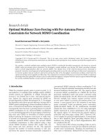
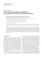
Figure 1: The MSE optimal kernel function for the family of locally
stationary processes
{x
α,β
(t), t ∈ Z,(α, β) ∈ Q}.
We see that the only difference b etween (10)and(5)is
that the summation in (5)ismadefors
= 1, , n and
t
= 1, , n whereas in (10), the summation is made for
s
= 1 − δ
q
, , n − δ
q
and t = 1 − δ
q
, , n − δ
q
. Since there
is only a small shift in the area for which the minimization
is performed, H
x
Q
−opt
will be approximately as optimal as

H
z
Q
−opt
on the family {z
q
(t), t ∈ Z,q ∈ Q}.
3. Examples
3.1. A Family of Locally Stationary Processes. We wil l now
consider a family of processes which are approximately
locally stationary. Let
{x
α,β
(t), t ∈ Z,(α, β) ∈ Q},where
Q
={(α, β):0<α≤ β ≤ 1} be a set of jointly
Gaussian random variables such that x
q
(t)andx
p
(s), q
/
= p,
are independent, E[x
α,β
(t)] = 0, x
α,β
(t) = 0forall
t/
∈ T

n
={1, , n}, r
α,β
(s, t) = E[x
α,β
(s)x
α,β
(t)
∗
] =
c
α,β
e
−(s−t)
2
/( αn)
2
e
−(s+t−n−1)
2
/( βn)
2
,wherec
α,β
is a normalization
factor c
α,β
= (

(s,t)∈T

2
n
e
−(s−t)
2
/( αn)
2
e
−(s+t−n−1)
2
/( βn)
2
)
−1/2
.
Each random process
{x
α,β
(t), t ∈ Z} is approximately
locally stationary in Silverman’s sense [13, 14]. Such pro-
cesses have been widely used in the literature, see for example
[10, 15]. Now, let Q be a random element of Q with uniform
distribution on Q, that is, the density function is 2 in Q and 0
otherwise. The MSE optimal kernel function for this family,
computed by the use of Theorem 1, is shown in Figure 1,
where n
= 64.
The optimal kernel function, H
x
Q

−opt
, for this family
can be compared with the optimal kernel funct ion for each
member of the family. Figure 2 shows the ratio between the
MSE when H
x
Q
−opt
is used and the MSE when H
x
α,β
−opt
is used
on realizations from
{x
α,β
(t), t ∈ Z},whereH
x
α,β
−opt
is the
MSE optimal kernel function for the process
{x
α,β
(t), t ∈ Z}.
4 EURASIP Journal on Advances in Signal Processing
0
0.5
1
0.10.20.30.40.50.60.70.80.91

1
1.08
1.2
1.5
2
2.5
β
α
MSE ratio
Figure 2: Ratio between MSE of t he MSE optimal kernel for the
family of locally stationary processes
{x
Q
(t)} and the MSE for the
kernel optimized for every (α, β)
∈ Q.
The kernel function H
x
Q
−opt
works remarkably well for every
member of the family, except when α is close to zero. In fact,
for more than 50% of the members of this family, the use of
the kernel function optimized for the whole family results in
less than 8% larger MSE than the kernel optimized for each
member.
3.2. A Family of Nonstationary AR(1)-Processes. Let e(t)
be a stationary AR(1)-process: e
θ
1

(t) = θ
1
e
θ
1
(t − 1) +
(t), |θ
1
| < 1, where {(t), t ∈ Z} is a white Gaussian
noise process with variance (1
−|θ
1
|)
1.5
. This process is
enveloped in order to get a nonstationary random process:
x
θ
1
, θ
2
(t) = e
θ
1
(t)e
−(t−n/2−0.5)
2
/( θ
2
n)

2
. As seen, the process x
θ
1
, θ
2
is described by two parameters, θ
1
and θ
2
. In this example,
we will compare two different kernels. The first one, H
rect-opt
,
is optimized using Theorem 1 for the rectangular parameter
set 0.5
≤ θ
1
≤ 0.9and0.5 ≤ θ
2
≤ 1. More formally, we apply
Theorem 1 on the family
{x
θ
1
, θ
2
(t), t ∈ Z,(θ
1
, θ

2
) ∈ Q},
where Q
= [0.5, 0.9] × [0.5, 1] and where Q is a random
element of Q with uniform distribution. The uniform
distribution is approximated with an equidistant grid of
point masses in order to simplify the integral expression.
The second kernel is a separable kernel function, that is,
a kernel function that can be separated into one function
dependent on k and one function dependent on τ.Such
kernels are well suited for covariance function estimation
of the random processes that we consider in this example.
We choose the separable kernel H
sep-opt
(k, τ) = h
1
(k)h
2
(τ),
where h
1
and h
2
are Hanning windows, each with a length
and amplitude that have been numerically MSE optimized
for (θ
1
, θ
2
) = (0.7, 0.75).

Thus, we now have two kernels, the first one optimized
on the rectangular space 0.5
≤ θ
1
≤ 0.9and0.5 ≤ θ
2
≤ 1
using Theorem 1, and the second one numerically optimized
in its four parameters (length of the two Hanning windows
and their amplitudes). We will now compare these for all
processes 0 <θ
1
< 1.5, 0 <θ
2
< 1. Note that we
−40 −30 −20 −100 10203040
−0.5
0
0.5
1
1.5
2
2.5
k
τ
= 0
τ =±5
τ
=±10
τ

=±15
H
X
Q
− opt
(k,τ)
Figure 3: The MSE optimal kernel function for the family of
nonstationary AR(1)-processes.
θ
2
θ
1
0.2
0.4 0.6
0.8
1
1.2
1.4
0.1
0.2
0.3
0.4
0.5
0.6
0.7
0.8
0.9
1
0.88
0.9

0.92
0.94
0.96
0.98
1
The separable kernel, H
sep
,
is numerically optimized at
this point.
The kernel, H
rect-opt
,is
optimized for the rectangular
area using Theorem 1.
Except for this region,
H
rect-opt
is MSE
superior to H
sep
.
Figure 4: The ratio between the MSE of the optimal kernel function
for the family of nonstationary AR(1)-processes and the MSE of
a separable kernel function. The first kernel has been optimized,
as given by Theorem 1, for the processes with parameters inside
the rectangle. The lengths and the amplitudes of the two Hanning
windows of the separable kernel have been optimized for the
parameter values at the circle. The black contour shows the border
where the two kernels give equally MSE. Outside this region the

kernel optimized as described in this paper is MSE superior to the
separable kernel.
include processes outside the rectangular, where H
rect-opt
is
optimized. The ratio between the MSE of the kernels is given
in Figure 4 as a function of the parameter space. We see that
the first kernel, H
rect-opt
, is better than the separable kernel
nearly everywhere.
EURASIP Journal on Advances in Signal Processing 5
k
−150
−100
−50
0
50
100
150
−150 −100 −50 0 50 100 150
−10
−5
0
5
10
τ
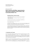
Figure 5: The MSE optimal kernel function for the family of
enveloped chirp processes.
3.3. A Family of Chirp Processes. In this example, we will

study measurements of heart rate variability (HRV), [16].
Such measurements are often modeled as an observed real-
ization from a nonstationary random process with stationary
mean. The second-order moments are considered to be
of greatest value from a medical perspective, [17]. Our
HRV measurements can be expected to have an increasing
frequency as the recording is made during an experiment
with increasing respiratory rate.
Our data consist of n
= 170 HRV measurements
with sampling rate 2 Hz. After the mean of the data has
been removed, we consider it to be an observation of
a nonstationary zero-meaned random process. In order
to estimate the covariance function of this process, we
use an estimator of the form (1), where we compute
the kernel function to be MSE optimal to the following
family of jointly Gaussian distributed enveloped chirps: let
{x
(α,β,γ)
(t), t ∈ Z,(α, β, γ) ∈ Q},wherex
(α,β,γ)
(t) =
Aw
γ
(t) sin(2πν
(α,β)
(t)t + ν
0
)forallt ∈ T
n

and 0 otherwise,
ν
(α,β)
(t) = αt/n + β, w
γ
(t) = 1/γ e
−(t−n/2−0.5)
2
/( γn)
2
, ν
0
is
a random variable uniformly distributed in [0, 2π), and A
is a Rayleigh-distributed random variable independent of
ν
0
.Theparametersα and β can be thought of as the raise
and starting point of the chirp frequency and γ as the
width of the envelope. We choose the a priori distribution
of the parameters to be uniform on
−0.1 ≤ α ≤ 0.1,
−0.25 ≤ β ≤ 0.25, 0.1 ≤ γ ≤ 1, but in order to
simplify the computations we approximate this distribution
with a uniform point distribution. The MSE optimal kernel
function is computed as described in Theorem 1 and can be
seen in Figure 5. As mentioned in the introduction, non-
parametr ic covariance function estimators are not guaran-
teed to be non-negative definite, [7]. We make the resulting
covariance matrix estimate non-negative definite by writing

the estimate as an eigenvalue decomposition and removing
the negative eigenvalues and their respective eigenvectors.
The corresponding Wigner spectr um is computed using
Jeong and Williams discrete Wigner representation, [4, 18].
0
0.05
0.1
0.15
0.2
0.25
0.3
0.35
0.4
0.45
0.5
Time (s)
20 40 60 80
Time (s)
20 40 60 80
Frequency (Hz)
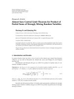
Figure 6: Left: Wigner distribution of HRV data. Right: Wigner
spectrum of the estimated covariance function.
It is shown in Figure 6 together with the Wigner distribution
of the data [2, 19].
4. Conclusions and Final Remarks
A non-parametric estimate of the covariance function of a
random process is often obtained by the use of a kernel
function. Different kernel functions have been proposed,
[8]. In order to favor one kernel over another, some prior
knowledge about the random process is needed. In this

paper, we have proved that the MSE optimal kernel function
for any parameterizable family of random processes can be
computed. In a few examples, we have demonstrated that the
resulting kernel can be close to optimal for all members of
the family. Moreover, the resulting kernels are often robust
in the sense that they also work well for nonmembers of the
family.
Appendix
Proof of Theorem 1
We would like to solve the following minimization problem:
H
x
Q
−opt
= arg min
H∈H
E
⎡
⎣

(
s,t
)
∈T
2
n



r

x
Q
(
s, t
)
− R
x
Q
;H
(
s, t
)



2
⎤
⎦
With τ = s − t:
= arg min
H∈H
E
⎡
⎣
n−1

τ=−n+1
min
(
n,n

−τ
)

t=max
(
1,1−τ
)
×



r
x
Q
(
t + τ, t
)
− R
x
Q
; H
(
t + τ, t
)



2
⎤
⎦

6 EURASIP Journal on Advances in Signal Processing
= arg min
H∈H

Q
n
−1

τ=−n+1
min
(
n,n
−τ
)

t=max
(
1,1−τ
)
× E




r
x
q
(
t + τ, t
)

− R
x
q
; H
(
t + τ, t
)



2

dF
Q

q

=
arg min
H∈H

Q
n
−1

τ=−n+1
min
(
n,n
−τ

)

t=max
(
1,1−τ
)
× E
⎡
⎣






r
x
q
(
t + τ, t
)
−
1
|K
τ
|

k∈K
τ
H

(
k, τ
)
× x
q
(
t + τ + k
)
x
q
(
t + k
)
∗






2
⎤
⎥
⎦
dF
Q

q

=

arg min
H∈H

Q
n
−1

τ=−n+1
min
(
n,n
−τ
)

t=max
(
1,1−τ
)
×E
⎡
⎣
−
r
x
q
(
t+τ, t
)
1
|K

τ
|

k∈K
τ
H
(
k, τ
)
∗
x
q
(
t+τ+k
)
∗
x
q
(
t+k
)
− r
x
q
(
t+τ, t
)
∗
1
|K

τ
|

k∈K
τ
H
(
k, τ
)
x
q
(
t+τ+k
)
x
q
(
t+k
)
∗
+
1
|K
τ
|
2

k
1
∈K

τ

k
2
∈K
τ
H
(
k
1
, τ
)
∗
H
(
k
2
, τ
)
x
q
(
t + τ + k
1
)
∗
× x
q
(
t+k

1
)
x
q
(
t+τ+k
2
)
x
q
(
t+k
2
)
∗
⎤
⎦
dF
Q

q

=
arg min
H∈H

Q
n
−1


τ=−n+1
min
(
n,n
−τ
)

t=max
(
1,1−τ
)
×
⎛
⎝
−r
x
q
(
t + τ, t
)
1
|K
τ
|

k∈K
τ
H
(
k, τ

)
∗
r
x
q
(
t + τ + k, t + k
)
− r
x
q
(
t + τ, t
)
∗
1
|K
τ
|

k∈K
τ
H
(
k, τ
)
r
x
q
(

t + τ + k, t + k
)
∗
+
1
|K
τ
|
2

k
1
∈K
τ

k
2
∈K
τ
H
(
k
1
, τ
)
H
(
k
2
, τ

)
∗
× ρ
x
q
(
t + k
1
, τ, t + k
2
, τ
)
⎞
⎠
dF
Q

q

.
(A.1)
We denote the target of minimization with F : H
→ R,
associate H with
R
2(2n
2
−2n+1)
, and we find the minima by
setting its derivative with respect to H(k, τ)

∗
to zero:
∂F
∂H
(
k, τ
)
∗
=

Q
min
(
n,n
−τ
)

t=max
(
1,1−τ
)
⎛
⎝
−
r
x
q
(
t + τ, t
)

1
|K
τ
|
r
x
q
(
t + τ + k, t + k
)
+
1
|K
τ
|
2

k
1
∈K
τ
H
(
k
1
, τ
)
×ρ
x
q

(
t + k
1
, τ, t + k, τ
)
⎞
⎠
dF
Q

q

=
0,
(A.2)
which concludes the proof.
Acknowledgments
This work was supported by the Swedish Research Council.
The first author would like to thank Johannes Siv
´
en at Lund
University for stimulating and valuable discussions.
References
[1] J. Sandberg and M. Hansson-Sandsten, “A comparison
between different discrete ambiguity domain definitions in
stochastic time-frequency analysis,” IEEE Transactions on
Signal Processing, vol. 57, no. 3, pp. 868–877, 2009.
[2] G. Matz and F. Hlawatsch, “Wigner dist ributions (nearly)
everywhere: time-frequency analysis of signals, systems, ran-
dom processes, signal spaces, and frames,” Signal Processing,

vol. 83, no. 7, pp. 1355–1378, 2003.
[3] M. B. Priestley, “Evolutionary spectra and non-stationary
processes,” Journal of the Royal Statistical Society B, vol. 27, no.
3, pp. 204–237, 1965.
[4] W. Martin, “Time-frequency analysis of random signals,” in
Proceedings of the IEEE International Conference on Acoustics,
Speech, and Signal Processing (ICASSP ’82), vol. 7, pp. 1325–
1328, 1982.
[5] R. Hyndman and M. Wand, “Nonparametric autocovariance
function estimation,” Australian Journal of Statistics, vol. 39,
pp. 313–325, 1997.
[6]D.Ruppert,M.P.Wand,U.Holst,andO.H
¨
ossjer, “Local
polynomial variance-function estimation,” Technometric s, vol.
39, no. 3, pp. 262–273, 1997.
[7] P. Hall, N. I. Fisher, and B. Hoffmann, “On the nonparametric
estimation of covariance functions,” The Annals of Statistics,
vol. 22, no. 4, pp. 2115–2134, 1994.
[8] M. G. Amin, “Spectral smoothing and recursion based on
the nonstationarity of the autocorrelation function,” IEEE
Transactions on Signal Processing, vol. 39, no. 1, pp. 183–185,
1991.
[9]A.M.SayeedandD.L.Jones,“Optimalkernelsfornon-
stationary spectral estimation,” IEEE Transactions on Signal
Processing, vol. 43, no. 2, pp. 478–491, 1995.
[10] P. Wahlberg and M. Hansson, “Kernels and multiple windows
for estimation of the Wigner-Ville spectrum of Gaussian
locally stationary processes,” IEEE Transactions on Signal
Processing, vol. 55, no. 1, pp. 73–84, 2007.

EURASIP Journal on Advances in Signal Processing 7
[11] P. Wahlberg and M. Hansson, “Optimal time-frequency
kernels for spectral estimation of locally stationary processes,”
in Proceedings of the IEEE Wor kshop on Statistical Signal
Processing, pp. 250–253, 2003.
[12] J. Sandberg and M. Hansson-Sandsten, “Optimal stochastic
discrete time-frequency analysis in the ambiguity and time-
lag domain,” Signal Processing, vol. 90, no. 7, pp. 2203–2211,
2010.
[13] R. A. Silverman, “Locally stationary random processes,” IRE
Transactions on Information Theory, vol. 3, pp. 182–187, 1957.
[14] R. A. Silverman, “A matching theorem for locally stationary
random processes,” Communications on Pure and Applied
Mathematics, vol. 12, pp. 373–383, 1959.
[15] P. Flandrin, Time-Frequency/Time Scale Analysis,Academic
Press, New York, NY, USA, 1999.
[16] E. Kristal-Boneh, M. Raifel, P. Froom, and J. Ribak, “Heart
rate variability in health and disease,” Scandinavian Journal of
Work, Environment and Health, vol. 21, no. 2, pp. 85–95, 1995.
[17] M. Hansson-Sandsten and P. J
¨
onsson, “Multiple window
correlation analysis of HRV power and respiratory frequency,”
IEEE Transactions on Biomedical Engineering, vol. 54, no. 10,
pp. 1770–1779, 2007.
[18] J. Jeong and W. J. Williams, “Alias-free generalized discrete-
time time-frequency distributions,” IEEE Transactions on
Signal Processing, vol. 40, no. 11, pp. 2757–2765, 1992.
[19] T.A.C.M.ClaasenandW.F.G.Mecklenbr
¨

auker, “The Wigner
distribution—a tool for time-frequency signal analysis. Part II:
discrete-time signals,” Philips Journal of Research, vol. 35, no.
4-5, pp. 276–300, 1980.