Báo cáo hóa học: " Research Article Parametric Adaptive Radar Detector with Enhanced Mismatched Signals Rejection Capabilities Chengpeng Hao,1 Bin Liu,2 Shefeng Yan,1 and Long Cai1" potx

Hindawi Publishing Corporation
EURASIP Journal on Advances in Signal Processing
Volume 2010, Article ID 375136, 11 pages
doi:10.1155/2010/375136
Research Article
Paramet ric Adaptive Radar Detector with Enhanced Mismatched
Signals Rejection Capabilities
Chengpeng Hao,
1
Bin Liu,
2
Shefeng Yan,
1
and Long Cai
1
1
Institute of Acoustics, Chinese Academy of Sc iences, Beijing 100190, China
2
Department of Electrical and Computer Engineering, Duke University, Durham, NC 27708, USA
Correspondence should be addressed to Chengpeng Hao,
Received 12 August 2010; Accepted 2 November 2010
Academic Editor: M. Greco
Copyright © 2010 Chengpeng Hao et al. This is an open access article distributed under the Creative Commons Attribution
License, which permits unrestricted use, distribution, and reproduction in any medium, provided the original work is properly
cited.
We consider the problem of adaptive signal detection in the presence of Gaussian noise with unknown covariance matrix. We
propose a parametric radar detector by introducing a design parameter to trade off the target sensitivity with sidelobes energy
rejection. The resulting detector merges the statistics of Kelly’s GLRT and of the Rao test and so covers Kelly’s GLRT and the Rao
test as special cases. B oth invariance properties and constant false alarm rate (CFAR) behavior for this detector are studied. At
the analysis stage, the performance of the new receiver is assessed and compared with several traditional adaptive detectors. The
results highlight better rejection capabilities of this proposed detector for mismatched signals. Further, we develop two two-stage

detectors, one of which consists of an adaptive matched filter (AMF) followed by the aforementioned detector, and the other
is obtained by cascading a GLRT-based Subspace Detector (SD) and the proposed adaptive detector. We show that the former
two-stage detector outperforms traditional two-stage detectors in terms of selectivity, and the latter yields more robustness.
1. Introduction
Adaptive detection of signals embedded in Gaussian or non-
Gaussian disturbance with unknown covariance matrix has
been an active research field in the last few decades. Several
generalized likelihood ratio test- (GLRT-) based methods are
proposed, which utilize secondary (training) data, that is,
data vectors sharing the same spectral properties, to form
an estimate of the disturbance covariance. In particular,
Kelly [1] derives a constant false alarm rate (CFAR) test
for detecting target signals known up to a scaling factor;
Robey et al. [2] develops a two-step GLRT design procedure,
called adaptive matched filter (AMF). Based on the above
methods, some improved approaches have been proposed,
for example, the non-Gaussian version of Robey’s adaptive
strategy in [3–6] and the extended targets version of Kelly’s
adaptive detection str ategy in [7]. In addition, considering
the presence of mutual coupling and near-field effects, De
Maio et al. [8] redevises Kelly’s GLRT detector and the AMF.
Most of the above methods work well, provided that
the exact knowledge of the signal array response vector
is available; however, they may experience a performance
degradation in practice when the actual steering vector is not
aligned with the nominal one. A side lobe mismatched signal
may appear subject to several causes, such as calibration
and pointing errors, imperfect antenna shape, and wavefront
distortions. To handle such mismatched signals, the Adaptive
Beamformer Orthogonal Rejection Test (ABORT) [9]is

proposed, which takes the rejection capabilities into account
at the design stage, introducing a tradeoff between the
detection performance for main lobe signals and rejection
capabilities for side lobe ones. The directivity of this detector
is in between that of the Kelly’s GLRT and the Adaptive
Coherence Estimator (ACE) [10, 11]. A Whitened ABORT
(W-ABORT) [12, 13] is proposed to address adaptive
detection of distributed targets embedded in homogeneous
disturbance via GLRT and the useful and fictitious signals
orthogonal in the whitened space, which has an enhanced
rejection capability for side lobe signals. Some alternative
approaches are devised [14–17], which basically depend on
constraining the actual signature to span a cone, whose
axis coincides with its nominal value. Moreover, in [18],
2 EURASIP Journal on Advances in Signal Processing
a detector based on the Rao test criterion is int roduced
and assessed. It is worth noting that the Rao test exhibits
discrimination capabilities of mismatched signals better than
those of the ABORT, although it does not consider a possible
spatial signature mismatch at the design stage.
From another point of view, increased robustness to
mismatch signals can be obtained by two-stage tunable
receivers that are formed by cascading two detectors (usually
with opposite behaviors), in which case, only data vectors
exceeding both detection thresholds will be declared as the
target bearings [19–23]. Remarkably, such solutions can
adjust directivity by proper selection of the two thresholds
to trade good rejection capabilities of side lobe signals
for an acceptable detection loss for matched signals. An
alternative approach to design tunable recei vers relies on

the parametric adaptive detectors, which allow us to trade
off target sensitivity with side lobes energy rejection via
tuning a design parameter [24, 25]. In particular, in [24],
Kalson devises a parametr ic detector obtained by merging
the statistics of Kelly’s GLRT and of the AMF, whereas in [25],
Bandiera et al. propose another parametric adaptive detector,
which is obtained by mixing the statistic of Kelly’s GLRT with
that of the W-ABORT.
In this paper, we attempt to increase the rejection
capabilities of tunable receivers and develop a novel adaptive
parametric detector, which is obtained by merging the
statistics of the Kelly’s GLRT and of the Rao test. We show
that the proposed detector is invariant under the group of
transformations defined in [26]. As a consequence, it ensures
the CFAR property with respect to the unknown covariance
matrix of the noise. The performance assessment, conducted
analytically for matched and mismatched signals, highlights
that specified with a appropriate design parameter the new
detector has better rejection capabilities for side lobe targets
than existing decision schemes. However, if the value of
the design parameter is bigger than or equals to unity, this
new detector leads to worse detection performance than
Kelly’s receiver. To circumvent this drawback, a two-stage
detector is proposed, which consists of the AMF followed
by the proposed paramet ric adaptive detector and can be
taken as an improved alternative of the two-stage detector in
[18]. We also give another two-stage detector with enhanced
robustness, which is obtained by cascading the GLRT-based
Subspace Detector (SD) [27] and the proposed parametric
adaptive receiver.

The paper is organized as follows. In the next section, we
formulate the problem and then propose the adaptive para-
metric detector. In Section 3, we analyze the performance
of the proposed receiver. We present two newly proposed
two-stage tunable detectors, respectively, in Sections 4 and
5. Section 6 contains conclusions and avenues for further
research. Finally, some analytical derivations are given in the
Appendix.
2. Problem Formulation and Design Issues
We assume that data are collected from N sensors and denote
by x
∈ C
N×1
the complex vector of the samples where the
presence of the useful signal is sought (primary data). As
customary, we also suppose that a secondary data set x
l
,
l
= 1, , K, is available (K ≥ N), that each of such snapshots
does not contain any useful target echo and exhibits the
same covariance matrix as the primary data (homogeneous
environment).
The detection problem at hand can be formulated in
terms of the following binary hypothesis test:
H
0
:
⎧
⎨

⎩
x = n,
x
l
= n
l
, l = 1, , K,
H
1
:
⎧
⎨
⎩
x = αp + n,
x
l
= n
l
, l = 1, , K,
(1)
where
(i) n and n
l
∈ C
N×1
, l = 1, , K, are independent,
complex, zero-mean Gaussian vectors with covari-
ance matrix given by
E


nn
†

=
E

n
l
n
†
l

=
M, l = 1, , K,(2)
where E[
·] denotes expectation and
†
conjugate
transposition;
(ii) p
∈ C
N×1
is the unit-norm steering vector of main
lobe target echo, which is possibly different from that
of the nominal steering vector p
0
;
(iii) α
∈ C is an unknown deterministic factor which
accounts for both target reflectivity and channel

effects.
The Rao test for the above problem [18]isgivenby
t
rao
=


x
†
S
−1
p
0


2
(
1+x
†
S
−1
x
)
p
†
0
S
−1
p
0


1+x
†
S
−1
x−


x
†
S
−1
p
0


2
/p
†
0
S
−1
p
0

,
(3)
where S
∈ C
N×N

is K times the sample covariance
matrix of the secondary data, that is, S
=

K
l
=1
x
l
x
†
l
.Itis
straightforward to show that t
rao
can be recast as
t
rao
=
t
2
glrt
t
amf

1 − t
glrt

=
t

glrt
t
amf

1 − t
glrt

t
glrt
=

1+x
†
S
−1
x −


x
†
S
−1
p
0


2
p
†
0

S
−1
p
0

−1
×


x
†
S
−1
p
0


2
(
1+x
†
S
−1
x
)

p
†
0
S

−1
p
0

,
(4)
EURASIP Journal on Advances in Signal Processing 3
where
t
amf
=


x
†
S
−1
p
0


2
p
†
0
S
−1
p
0
(5)

is the AMF decision statistic, and
t
glrt
=


x
†
S
−1
p
0


2
(
1+x
†
S
−1
x
)

p
†
0
S
−1
p
0


(6)
is the decision statistic of Kelly’s GLRT.
Comparing t
rao
with t
glrt
, we propose a new detector,
termed KRAO in the following. Its decision statistic is
t
krao
=

1+x
†
S
−1
x −


x
†
S
−1
p
0


2
p

†
0
S
−1
p
0

−(2ρ−1)
×


x
†
S
−1
p
0


2
(
1+x
†
S
−1
x
)

p
†

0
S
−1
p
0

(7)
or, equivalently
t
krao
=
⎡
⎣
t
glrt
t
amf

1 − t
glrt

⎤
⎦
(2ρ−1)
t
glrt
,
(8)
where ρ is the design parameter.
It is clear that our detector covers Kelly’s GLRT and the

Rao test as special cases, respectively, when ρ
= 0.5and
ρ
= 1. Moreover, since t
krao
canbeexpressedinterms
of the maximal invariant statistic ( t
amf
, t
glrt
), it is invariant
with respect to the transformations defined in [26]. As a
consequence, it ensures the CFAR property with respect to
the unknown covariance matrix of the noise.
3. Performance Assessment
In this section, we derive an analytic expression of P
fa
and P
d
and then present illustrative examples for KRAO. Specifically,
in derivation of P
d
, we consider a general case, in which the
signal in the primary data vector is not commensurate with
the nominal steering vector, that is we consider detection
performance for mismatched signal. To this end, we first
introduce the random variable
β
=


1+x
†
S
−1
x −


x
†
S
−1
p
0


2
p
†
0
S
−1
p
0

−1
(9)
and then consider the equivalent form of Kelly’s statistic

t
glrt

= t
glrt
/(1 − t
glrt
). Thus, t
krao
can be expressed to be
t
krao
= β
2ρ−1

t
glrt
1+

t
glrt
. (10)
3.1. P
fa
of the KRAO. Under H
0
hypothesis, the following
statements hold [21]:
(i) given β,

t
glrt
is ruled by the complex central F-

distribution with 1, K
− N + 1 degrees of freedom,
namely,

t
glrt
∼ CF
1,K−N+1
;
(ii) β is a complex central beta distribution random
variable (rv) with K
−N +2, N −1 degrees of freedom,
namely, β
∼ Cβ
K−N+2,N−1
.
Therefore, the KRAO associated P
fa
satisfies
P
fa

ρ, η

=
P

β
2ρ−1


t
glrt
1+

t
glrt
>η; H
0

=
P


t
glrt
>
η
β
2ρ−1
− η
; H
0

=

1
0

1 − F
0


η
ε
2ρ−1
− η

f
β
(
ε
)
dε,
(11)
where η is the threshold set beforehand, whose value depends
on the value of P
fa
, f
β
(·) is the probability density function
(pdf) of the rv β
∼ Cβ
K−N+2,N−1
,andF
0
(·) is the cumulative
distribution function (cdf) of the rv

t
glrt
∼ CF

1,K−N+1
,given
β. Then it follows
P


t
glrt
1+

t
glrt
>
η
β
2ρ−1
; H
0

=
⎧
⎪
⎪
⎨
⎪
⎪
⎩
0, β
2ρ−1
≤ η

P


t
glrt
>
η
β
2ρ−1
− η
; H
0

, β
2ρ−1
>η.
(12)
Substituting (12) into (11) followed by some algebra, it
yields
(i) ρ
≥ 0.5andη ≥ 1
P
fa

ρ, η

=
0,
(13)
(ii) ρ>0.5and0

≤ η<1
P
fa

ρ, η

=

1
η
1/(2ρ−1)

1 − F
0

η
ε
2ρ−1
− η

f
β
(
ε
)
dε, (14)
(iii) 0
≤ ρ<0.5andη ≥ 1
P
fa


ρ, η

=

η
1/(2ρ−1)
0

1 − F
0

η
ε
2ρ−1
− η

f
β
(
ε
)
dε,
(15)
(iv) 0
≤ ρ ≤ 0.5and0≤ η<1
P
fa

ρ, η


=

1
0

1 − F
0

η
ε
2ρ−1
− η

f
β
(
ε
)
dε. (16)
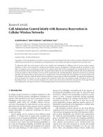
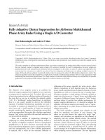
For the reader ease, Figure 1 shows the contour plots
for the KRAO corresponding to different values of P
fa
,as
functions of the threshold pairs (ρ, η), N
= 8, and K =
24. All curves have been obtained by means of numerical
integration techniques.
4 EURASIP Journal on Advances in Signal Processing
0 0.1 0.2 0.3 0.4 0.5 0.6

0
0.2
0.4
0.6
0.8
1
ρ
η
P
fa
= 10
−1
P
fa
= 10
−2
P
fa
= 10
−3
P
fa
= 10
−4
Figure 1: Contours of constant P
fa
for the KRAO versus η and ρ
with N
= 8, K = 24.
3.2. P

d
of the KRAO. Now we consider hypothesis H
1
.
Denote φ the ang le between p and p
0
in the whitened-
dimensional data space, that is,
cos
2
φ =


p
†
M
−1
p
0


2

p
†
M
−1
p



p
†
0
M
−1
p
0

.
(17)
The term cos
2
φ is a measure of the mismatch between p and
p
0
. Its value is one for the matched case w here p = p
0
,and
less than one otherwise. A small value of cos
2
φ implies a large
mismatch between the steering vector and signal. In this case,
due to the useful signal components, distributions of

t
glrt
and
β are given in [23]:
(i) given β,


t
glrt
is ruled by the complex noncentral F-
distribution with 1, K
− N + 1 degrees of freedom
and noncentrality parameter
δ
2
φ
= βSNR cos
2
φ,
(18)
namely,

t
glrt
∼ CF
1,K−N+1
(δ
φ
), where SNR =
|
α|
2
p
†
M
−1
p is the total available signal-to-noise

ratio;
(ii) β is a complex noncentral beita distribution rv with
K
−N +2, N −1 degrees of freedom and noncentrality
parameter
δ
2
β
= SNR sin
2
φ,
(19)
namely, β
∼ Cβ
K−N+2,N−1
(δ
β
).
Then P
d
is given by
P
d

φ

= P

β
2ρ−1


t
glrt
1+

t
glrt
>η; H
1

=

1
0

1 − F
1

η
ε
2ρ−1
− η

f
β
(
ε
)
dε,
(20)

where f
β
(·) is the pdf of the rv β ∼ Cβ
K−N+2,N−1
(δ
β
), and
then, given β, F
1
(·) is the cdf of the rv

t
glrt
∼ CF
1,K−N+1
(δ
φ
).
Similarly as before (in Section 3.1), we have
(i) ρ
≥ 0.5andη ≥ 1
P
d

φ

=
0,
(21)
(ii) ρ>0.5and0

≤ η<1
P
d

φ

=

1
η
1/(2ρ−1)

1 − F
1

η
ε
2ρ−1
− η

f
β
(
ε
)
dε, (22)
(iii) 0
≤ ρ<0.5andη ≥ 1
P
d


φ

=

η
1
/(2ρ−1)
0

1 − F
1

η
ε
2ρ−1
− η

f
β
(
ε
)
dε,
(23)
(iv) 0
≤ ρ ≤ 0.5and0≤ η<1
P
d


φ

=

1
0

1 − F
1

η
ε
2ρ−1
− η

f
β
(
ε
)
dε. (24)
In the case of a perfect match, δ
β
is equal to zero. As
a consequence, β is distributed as a complex central beta
distribution random variable with K
− N +2,N −1degrees
of freedom, and

t

glrt
is ruled by the complex noncentral
F-distribution with 1, K
− N + 1 degrees of freedom and
noncentrality parameter
δ
2
0
= βSNR.
(25)
3.3. Performance Analysis. In this subsection, we present
numerical examples to illustrate the performance of the
KRAO. The curves are obtained by numerical integration and
the probability of false alarm is set to 10
−4
.
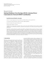
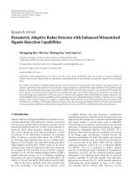
One can see the influence of the design parameter ρ
in Figures 2 and 3, where the P
d
of the KRAO is plotted
versus the SNR, considering both the case of a perfect
match between the actual steering vector and the nominal
one, namely, cos
2
φ = 1, and the case where there is
a misalig nment between the two aforementioned vectors,
more precisely cos
2
φ = 0.7. Specifically, Figures 2 and 3
correspond to ρ

≥ 0.5andρ ∈ [0, 0.5], respectively. From
Figure 2, we see that the curves associated w ith the KRAO
are in between that of Kelly’s GLRT and that of the Rao test
when ρ
∈ (0.5, 1.0), and that the KRAO outperforms the Rao
test in terms of selectivity for ρ>1. However, it is also shown
that the amount of detection loss for matched signals and
sensitivity to mismatched signals depend upon the design
parameter ρ. More specifically, a larger value of ρ leads to
better rejection capabilities of the side lobe signals and the
larger detection loss for matched signals. On the other hand,
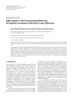
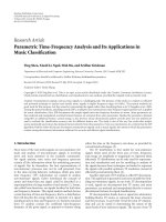
Figure 3 shows that, when ρ
∈ [0, 0.5),asmallervalueofρ
renders the performance less sensitive to mismatched signals.
In another word, robustness to mismatched signals can be
increased by setting ρ
∈ [0, 0.5). In summary, different values
of ρ represent different compromises between the detection
EURASIP Journal on Advances in Signal Processing 5
5 10152025
0.1
0.2
0.3
0.4
0.5
0.6
0.7
0.8
0.9
1

SNR (dB)
P
d
Kelly’s GLRT
Rao test
KRAO: ρ
= 0.7
KRAO: ρ
= 0.9
KRAO: ρ
= 1.2
KRAO: ρ
= 1.4
cos
2
φ = 1
cos
2
φ = 0.7
Figure 2: P
d
versus SNR for the KRAO, N = 8, K = 24, and ρ ≥ 0.5.
and the rejection performance. So the appropriate value of ρ
is selected based on the system needs.
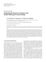
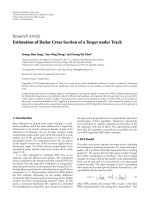
In Figures 4 and 5, we compare the KRAO to the ACE,
the ABORT, and Bandiera’s detector (KWA) [25]forN
= 16,
K
= 32, and under the constraint that the loss with respect
to Kelly’s GLRT is practically the same for the perfectly

matched case. For sake of completeness, we review these
CFAR detectors in the following:
t
ace
=


x
†
S
−1
p
0


2

p
†
0
S
−1
p
0

(
x
†
S
−1

x
)
,
t
abort
=
1+|x
†
S
−1
P
0
|
2
/p
†
0
S
−1
P
0
2+x
†
S
−1
x
,
t
kwa
=

1+x
†
S
−1
x

1+x
†
S
−1
x −


x
†
S
−1
p
0


2
/(p
†
0
S
−1
p
0
)


2γ
,
(26)
where γ is the design parameter of the KWA. From Figures
4 and 5, it is clear that the KRAO is superior to the KWA in
rejecting side lobe signals with ρ
= γ +0.1 It is also clear
that, with a proper choice of ρ, the KRAO outperforms the
ACE and the ABORT in terms of selectivity. Other simulation
results not reported here, in order not to burden too much
the analysis, have shown that the above results are still valid
for N
= 8andK = 24.
4. Two-Stage Detector Based on the KRAO
In this section, we propose a two-stage algorithm, aiming at
compensating the matched detection performance loss for
the KRAO with ρ
≥ 1. Briefly, this is obtained by cascading
the AMF and the KRAO (ρ
≥ 1). We term this two-stage
detector KRAO Adaptive Side lobe Blanker (KRAO-ASB).
This detector generalizes the two-stage Rao test (AMF-RAO)
Kelly’s GLRT
KRAO: ρ
= 0
KRAO: ρ
= 0.1
KRAO: ρ
= 0.2

KRAO: ρ
= 0.3
KRAO: ρ
= 0.4
5 10152025
0.1
0.2
0.3
0.4
0.5
0.6
0.7
0.8
0.9
1
SNR (dB)
P
d
cos
2
φ = 1
cos
2
φ = 0.7
0
Figure 3: P
d
versus SNR for the KRAO, N = 8, K = 24, and ρ ∈
[0, 0.5].
KRAO

KWA
ACE
cos
2
= 0.8
cos
2
φ =1
5 10152025
0
0.1
0.2
0.3
0.4
0.5
0.6
0.7
0.8
0.9
1
SNR (dB)
P
d
Figure 4: P
d
versus SNR for the KRAO with ρ = 0.9, the KWA with
γ
= 0.8, and the ACE, N = 16, K = 32.
[18]forρ = 1. We now summarize the implementation of
the proposed detector as below:

t
amf
≷ η
a
>η
a
−−→ t
krao
≷ η
k
>η
k
−−→ H
1
↓≤ η
a
↓≤ η
k
H
0
H
0
,
(27)
where η
a
and η
k
form the threshold pair, which are set in
such a way that the desired P

fa
is available. Observe that
the KRAO-ASB is invariant to the group of transformations
given in [26], due to the fact that t
krao
can be expressed
6 EURASIP Journal on Advances in Signal Processing
in terms of the maximal invariant statistic (t
amf
, t
glrt
). It is
thus not surpr ising that the KRAO-ASB ensures the CFAR
property with respect to the disturbance covariance matrix
M. In what follows, we derive the closed-form expressions for
P
fa
and P
d
of KRAO-ASB. Given a stochastic representation
for t
amf
[20]:
t
amf
=

t
glrt
β

,
(28)
the P
fa
follows to be
P
fa

η
a
, η
k
, ρ

=
P

t
amf
>η
a
, t
krao
>η
k
; H
0

=
P



t
glrt
β
>η
a
, β
2ρ−1

t
glrt
1+

t
glrt
>η
k
; H
0

=
P


t
glrt
>max

βη

a
,
η
k
β
2ρ−1
− η
k

; H
0

.
(29)
Note that
P
fa

η
a
, η
k
, ρ

=
⎧
⎪
⎪
⎪
⎨

⎪
⎪
⎪
⎩
0, β ≤ η
1/(2ρ−1)
k
,
max

βη
a
,
η
k
β
2ρ−1
− η
k

, β>η
1/(2ρ−1)
k
.
(30)
Consequently,
P
fa

η

a
, η
k
, ρ

=

1
η
1/(2ρ−1)
k
P


t
glrt
>max

xη
a
,
η
k
x
2ρ−1
− η
k

|
β = x; H

0

×
f
β
(
x
)
dx
=

1
η
1/(2ρ−1)
k

1 − F
0

max

xη
a
,
η
k
x
2ρ−1
− η
k


f
β
(
x
)
dx,
(31)
where f
β
(·) is pdf of the rv β ∼ Cβ
K−N+2,N−1
,andF
0
(·) is the
cdfoftherv

t
glrt
∼ CF
1,K−N+1
,givenβ. Then, we consider the
standard algebra
max

xη
a
,
η
k

x
2ρ−1
− η
k

=
⎧
⎪
⎪
⎨
⎪
⎪
⎩
xη
a
, x>σ,
η
k
x
2ρ−1
− η
k
, x ≤ σ,
(32)
where σ is the positive root to the equation
η
a
x
2ρ−1
− η

a
η
k
x −η
k
= 0
(33)
and can be obtained via Newton’s method. Substituting (32)
into ( 31) and performing some algebra, it yields that
(i) if η
a
≤ η
k
/(1 − η
k
), then σ ≥ 1
P
fa

η
a
, η
k
, ρ

=

1
η
1/(2ρ−1)

k

1 − F
0

η
k
x
2ρ−1
− η
k

f
β
(
x
)
dx,
(34)
namely, the two-stage detector achieves the same
performance as that of the KRAO test;
KRAO
KWA
cos
2
= 0.8
5 10152025
0.1
0.2
0.3

0.4
0.5
0.6
0.7
0.8
0.9
1
SNR (dB)
P
d
0
cos
2
φ = 1
ABORT
Figure 5: P
d
versus SNR for the KRAO with ρ = 0.7, the KWA with
γ
= 0.6, and the ABORT, N = 16, K = 32.
(ii) if η
a
>η
k
/(1 − η
k
), then σ<1
P
fa


η
a
, η
k
, ρ

=

σ
η
1/(2ρ−1)
k

1 − F
0

η
k
x
2ρ−1
− η
k

f
β
(
x
)
dx
+


1
σ

1 − F
0

xη
a

f
β
(
x
)
dx.
(35)
It is worth noting that there exist an infinite set of infinite
triplets (η
a
, η
k
, ρ) that result in the same P
fa
. Figure 6 shows
the contour plots corresponding to different values of P
fa
,
as functions of (η
a

, η
k
)forN = 8, K = 24, and ρ = 1.2. It
is shown that this detector provides a compromise between
the detection and the rejection performance and degenerates
to the AMF as η
k
= 0, and the KRAO when η
a
= 0. So
the appropriate operating point can be selected based on the
system requirements.
For H
1
hypothesis, the derivation process is similar. In
detail, if η
a
≤ η
k
/(1 − η
k
), P
d
is the same as for the KRAO
test; otherwise, it can be evaluated by
P
d

φ


=

σ
η
1/(2ρ−1)
k

1 − F
1

η
k
x
2ρ−1
− η
k

f
β
(
x
)
dx
+

1
σ

1 − F
1


xη
a

f
β
(
x
)
dx,
(36)
where f
β
(·) is the pdf of the rv β ∼ Cβ
K−N+2,N−1
(δ
β
), and
F
1
(·) is the cdf of the rv

t
glrt
∼ CF
1,K−N+1
(δ
φ
), given β.
The matched detection performances of the KRAO-ASB,

the KRAO, and the AMF are analyzed in Figure 7,withN
=
8, K = 24, ρ = 1.2, and P
fa
= 10
−4
. For KRAO-ASB, we
show the curve corresponding to the threshold setting that
returns the minimum loss with respect to the Kelly’s GLRT.
EURASIP Journal on Advances in Signal Processing 7
0 0.05 0.1 0.15 0.2 0.25
0.3
0
0.2
0.4
0.6
0.8
1
P
fa
= 10
−1
P
fa
= 10
−2
P
fa
= 10
−3

P
fa
= 10
−4
Threshold for the AMF
Threshold for the KRAO
Figure 6: Contours of constant P
fa
for the KRAO-ASB with N = 8,
K
= 24, and ρ = 1.2.
The curves highlight that for small-medium SNR values,
the KRAO-ASB yields better detection performance than
that obtained by performing either the AMF or the KRAO
operating alone. We argue that this behavior results from
the capability of the KRAO-ASB algorithm in combining
information from both single detectors. Similar results for
existing two-stage detectors refer to [18–21].
In Figures 8 and 9, we compare the KRAO-ASB
(equipped with ρ
= 1.2) to the two-stage detector based
on the KWA (KWAS-ASB) [25](affiliated w ith γ
= 1.1)
and the AMF-RAO. The threshold pairs correspond to the
most selective case and entail a l oss for matched signals of
about 1 dB with respect to the Kelly’s GLRT at P
d
= 0.9
and P
fa

= 10
−4
. Figure 8 refers to N = 8andK = 24,
and Figure 9 assumes N
= 16 and K = 32. As it can be
seen, the KRAO-ASB exhibits better rejection capabilities of
mismatched signals than the KWAS-ASB and the AMF-RAO
for the considered system parameters.
5. Improved Two-Stage D etector Based on
the KRAO
In order to increase the robustness to mismatched signals of
the KRAO-ASB, we propose another two-stage detector. This
detector is the same as KRAO-ASB, except that the AMF is
replaced by a SD. The resulting statistic is
t
sd
=
x
†
S
−1
H

H
†
S
−1
H

−1

H
†
S
−1
x
1+x
†
S
−1
x
,
(37)
where H
= [v ···v
r−1
] ∈ C
N×r
is a full-column-rank matrix
(r
≥ 1). The choice of H = [s(0), s(π/360)] makes this
detector robust in a homogeneous environment [21]. The
vector s(θ) is defined as follows:
s
(
θ
)
=
1
√
N


1, e
j(2πd/λ)sin θ
, , e
j(N−1)(2πd/λ)sin θ

T
,
(38)
where λ is the radar operating wavelength, d is the interele-
ment spacing, and T denotes transposition.
This detector, which we term Subspace-based and KRAO
Adaptive Side lobe Blanker (SKRAO-ASB), can be pictorial ly
described as follows:
t
sd
≷ η
s
>η
s
−−→ t
krao
≷ η
k
>η
k
−−→ H
1
↓≤ η
s

↓≤ η
k
H
0
H
0
,
(39)
where η
s
and η
k
form the threshold pair which should be
set beforehand to guarantee that the overall desired P
fa
is
available. We then derive closed-form expressions for P
fa
and P
d
of the KRAOS-ASB. First, we replace t
sd
with the
equivalent decision statistic

t
sd
= 1/(1 − t
sd
). It is shown that

the following identities hold for

t
sd
and t
krao
(see derivation
in Appendix):

t
sd
=
(
1+c
)

t
glrt
,
t
krao
=

1
1+b + c + bc

2ρ−1

t
glrt

1+

t
glrt
.
(40)
Then, under H
0
hypothesis [23]:
(i) given b and c,

t
glrt
is ruled by the complex central F-
distribution with 1, K
− N + 1 degrees of freedom,
namely,

t
glrt
∼ CF
1,K−N+1
;
(ii) b is a complex central F-distribution random variable
(rv) with N
− r, K − N + r + 1 degrees of freedom,
namely, b
∼ CF
N−r,K−N+r+1
;

(iii) c obeys the complex central F-distribution with r
−
1, K − N + 2 degrees of freedom, namely, c ∼
CF
r−1,K−N+2
;
(iv) b and c are statistically independent rv’s.
Therefore, the P
fa
of the SKRAO-ASB can be expressed
as
P
fa

η
s
, η
r
, ρ

=
P


t
sd
> η
s
, t
krao

>η
k
; H
0

=

∞
0

1 − F
0

max


η
s
1+k
− 1,
η
k
(
1+ε + k + εk
)
1−2ρ
− η
k

× f

b
(
ε
)
f
c
(
k
)
dεdk,
(41)
where
η
s
= 1/(1 − η
s
), f
b
(·) is the pdf of the rv b ∼
CF
N−r,K−N+r+1
, f
c
(·) is the pdf of the rv c ∼ CF
r−1,K−N+2
,
and F
0
(·) is the cdf of the r v


t
glrt
∼ CF
1,K−N+1
,givenb
and c. As can be seen from (41), the P
fa
of the SKRAO-
ASB depends on the threshold pairs (
η
s
, η
k
) and the design
parameter ρ, as a consequence of which, the SKRAO-ASB
possesses the constant false alarm rate (CFAR) property with
respect to the disturbance covariance matrix M.
For hypothesis H
1
, we assume that the first column of H
is p
0
, then perform QR factorization to M
−1/2
H:
M
−1/2
H = H
0
R

H
(42)
8 EURASIP Journal on Advances in Signal Processing
KRAO-ASB
AMF
KRAO
5 101520
0.1
0.2
0.3
0.4
0.5
0.6
0.7
0.8
0.9
1
SNR (dB)
P
d
0
Figure 7: Matched P
d
versus SNR for the KRAO-ASB, the KRAO,
and the AMF with N
= 8, K = 24, and ρ = 1.2.
with H
0
∈ C
N×r

being a slice of unitary matrix, namely,
H
†
0
H
0
= I
r
,andR
H
∈ C
r×r
an invertible upper triangular
matrix. Then we define a unitary matrix U that rotates the
r orthonormal columns of H
0
into the first r elementary
vectors, that is,
UH
0
=
⎡
⎣
I
r
0
(N−r)×r
⎤
⎦
(43)

and, in particular,
UM
−1/2
p
0
=

p
†
0
M
−1
p
0
e
1
,
(44)
where e
1
is the N-dimensional column vector whose first
entry is equal to one and the remainings are zero. It turns
out that the whitened data vector z
= UM
−1/2
x is distributed
as [28]
z : CN
N
⎛

⎜
⎜
⎜
⎝
α

p
†
M
−1
p
⎡
⎢
⎢
⎢
⎣
e
jϕ
cos φ
h
B
0
sin φ
h
B
1
sin φ
⎤
⎥
⎥

⎥
⎦
, I
N
⎞
⎟
⎟
⎟
⎠
, (45)
where h
B
0
∈ C
(r−1)×1
, h
B
1
∈ C
(N−r)×1
with


h
B
0


2
+



h
B
1


2
= 1,
(46)
where
·denotes the Euclidean norm of a vector. Then
because of the useful signal components, the distr ibutions of
t, b and c are given in [23]:
(i) given b and c,

t
glrt
is ruled by the complex noncentral
F-distribution with 1, K
− N + 1 degrees of freedom
and noncentrality parameter
δ
2
φ
=
SNRcos
2
φ
1+b + c + bc

,
(47)
namely,

t
glrt
∼ CF
1,K−N+1
(δ
φ
);
cos
2
= 0.8
5 10152025
0.1
0.2
0.3
0.4
0.5
0.6
0.7
0.8
0.9
1
SNR (dB)
P
d
KRAO-ASB
AMF-RAO

KWAS-ASB
0
cos
2
φ = 1
Figure 8: P
d
versus SNR for the KRAO-ASB with ρ = 1.2, the
KWAS-ASB with γ
= 1.1, and the AMF-RAO, N = 8, K = 24.
(ii) b is a complex noncentral F-distribution rv with N −
r, K −N + r +1 degrees of freedom and noncentrality
parameter
δ
2
b
= SNRsin
2
φ


h
B
1


2
,
(48)
namely, b

∼ CF
N−r,K−N+r+1
(δ
b
);
(iii) given b, c obeys the complex noncentral F-
distribution with r
−1, K −N + 2 degrees of freedom
and noncentrality parameter
δ
2
c
=
SNRsin
2
φ


h
B
0


2
1+b
,
(49)
namely, c
∼ CF
r−1,K−N+2

(δ
c
).
Now, it is easy to see that the P
d
for the SKRAO-ASB can be
expressed as
P
d

φ

=
P


t
sd
> η
s
, t
rao
>η
r
; H
1

=

∞

0

1 − F
1
×

max


η
s
1+κ
−1,
η
k
(
1+ε+k+εk
)
1−2ρ
−η
k

×
f
c|b
(
κ
| b = ε
)
f

b
(
ε
)
dεdκ,
(50)
where f
b
(·) is the pdf of the rv b ∼ CF
N−r,K−N+r+1
(δ
b
),
f
c|b
(·|·) is the pdf of the rv c ∼ CF
r−1,K−N+2
(δ
c
), given
b,andF
1
(·)isthecdfof

t
glrt
∼ CF
1,K−N+1
(δ
φ

), given b and c.
In Figures 10 and 11, we plot P
d
versus φ (measured in
degrees) for the SKRAO-ASB and the KRAO-ASB for N
= 8,
EURASIP Journal on Advances in Signal Processing 9
cos
2
= 0.8
5 10152025
0.1
0.2
0.3
0.4
0.5
0.6
0.7
0.8
0.9
1
SNR (dB)
P
d
KRAO-ASB
AMF-RAO
KWAS-ASB
0
cos
2

φ = 1
Figure 9: P
d
versus SNR for the KRAO-ASB with ρ = 1.2, the
KWAS-ASB with γ
= 1.1, and the AMF-RAO, N = 16, K = 32.
0.1
0.2
0.3
0.4
0.5
0.6
0.7
0.8
0.9
1
P
d
0
246810
12
φ (degrees)
KRAO
0
SD
Figure 10: P
d
versus φ for the SKRAO-ASB with N = 8, K = 24,
ρ
= 1.2, H = [s(0), s(π/360)], and SNR = 18 dB.

K = 24, ρ = 1.2, H = [s(0), s(π/360)], P
fa
= 10
−4
,
and SNR
= 18 dB. The different curves of each plot refer
to different threshold pairs. From Figures 10 and 11,itis
clear that the SKRAO-ASB can ensure better robustness with
respect to the KRAO-ASB, due to the first stage (the SD),
which is less sensitive than the AMF to mismatched signals.
It is also clear that, for a given value of ρ, the SKRAO-ASB
and the KRAO-ASB exhibit the same capability to reject side
lobe signals, due to fact that the second stage (the KRAO) is
the same.
Finally, we compare the SKRAO-ASB and the KRAO-ASB
in terms of computational complexity. We focus on the first
stage of each detector, since the second stage of each detector
is to be computed only if the fist stage declares a detection.
Observe that the AMF does not require the on-line inversion
0.1
0.2
0.3
0.4
0.5
0.6
0.7
0.8
0.9
1

P
d
0
246810
12
φ (degrees)
KRAO
AMF
0
Figure 11: P
d
versus φ for the KRAO-ASB with N = 8, K = 24,
ρ
= 1.2, and SNR = 18 dB.
of the matrix H
†
S
−1
H (r>1) and the computation of the
extra term 1 + x
†
S
−1
x, which are necessary to implement
the SD decision statistic. It is thus apparent that the KRAO-
ASB is faster to implement than the SKRAO-ASB. Anyway,
resorting to the usual Landau notation, the SKRAO-ASB
involves O(KN
2
)+O(N) floating-point operations (flops),

whereas the KRAO-ASB requires O(KN
2
)flops.
6. Conclusions
In this paper, we consider the problem of adaptive signal
detection in the presence of Gaussian noise with unknown
covariance matrix. Contributions in this paper are summa-
rized as follows.
(i) We propose a new parametric radar detector, KRAO,
by merging the statistics of the Kelly’s GLRT test and
of the Rao test. We discuss its invariance and CFAR
property. We derive the closed-form expressions for
the probability of false alarm and the probability of
detection in matched and mismatched cases.
(ii) We demonstrate performance of KRAO via simula-
tions. Numerical results show that, with a properly
selected value for the design parameter, the pro-
posed KRAO can yield better rejection capabilities of
mismatched signals than its counterparts. However,
when the sensitivity parameter is greater than or
equal to unity, it has a nonnegligible loss for matched
signals compared with Kelly’s GLRT.
(iii) To compensate the matched detection performance
of the KRAO, we propose a two-stage detector
consisting of an adaptive matched filter followed by
the KRAO. We show that such a two-stage detector
has desirable property in terms of selectiv ity. Its
invariance and CFAR property have been studied.
(iv) To increase the robustness of the aforementioned
two-stage detector, we introduce another two-stage

10 EURASIP Journal on Advances in Signal Processing
detector by cascading a GLRT-based subspace detec-
tor and the KRAO. It possesses the CFAR property
with respect to the unknown covariance matrix of
the noise and it can guarantee a wider range of
directivity values with respect to aforementioned
two-stage detector.
Further work will involve the analysis of the proposed
tunable receivers in a partially homogeneous (Gaussian)
environment scenario, that is, when the noise covariance
matrices of the primary and the secondar y data have the
same structure but are at different power levels. It is also
needed to investigate these tunable receivers in a clutter-
dominated non-Gaussian scenario.
Appendix
Stochastic Representations of
the KRAO and the SD
In this appendix, we come up with suitable stochastic
representations for t
krao
and

t
sd
. First, we can recast t
krao
as
follows:
t
krao

= β
2ρ−1

t
glrt
1+

t
glrt
,(A.1)
where β is given by (9). It is shown that β is distributed as a
complex noncentral beta rv [28] and can be expressed as the
functions of two independent rv’s b and c [21], that is,
β
=
1
1+b + c + bc
.
(A.2)
It follows that t
krao
can be recast as
t
krao
=

1
1+b + c + bc

2ρ−1


t
glrt
1+

t
glrt
. (A.3)
As to the GLRT-based subspace detector, it is shown that [21]

t
sd
=
(
1+c
)


t
glrt
+1

. (A.4)
A deeper discussion on the statistical characterization of b
and c can be found in [23].
Acknowledgments
The authors are very grateful to the anonymous referees for
their many helpful comments and constructive suggestions
on improving the exposition of this paper. This work was
supported by the National Natural Science Foundation of

China under Grant no. 60802072.
References
[1] E. J. Kelly, “An adaptive detection algorithm,” IEEE Transac-
tions on Aerospace and Electronic Systems,vol.22,no.2,pp.
115–127, 1986.
[2] F. C. Robey, D. R. Fuhrmann, E. J. Kelly, and R. Nitzberg, “A
CFAR adaptive matched filter detector,” IEEE Transactions on
Aerospace and Electronic Systems, vol. 28, no. 1, pp. 208–216,
1992.
[3] M. Greco, F. Gini, and M. Diani, “Robust CFAR detection of
random signals in compound-Gaussian clutter plus thermal
noise,” IEE Proceedings: Radar, Sonar and Navigation, vol. 148,
no. 4, pp. 227–232, 2001.
[4] A. Younsi, M. Greco, F. Gini, and A. M. Zoubir, “Performance
of the adaptive generalised matched subspace constant false
alarm rate detector in non-Gaussian noise: an experimental
analysis,” IET Radar, Sonar and Navigation, vol. 3, no. 3, pp.
195–202, 2009.
[5] A. de Maio, G. Alfano, and E. Conte, “Polar ization diversity
detection in compound-Gaussian clutter,” IEEE Transactions
on Aerospace and Electronic Systems, vol. 40, no. 1, pp. 114–
131, 2004.
[6] X. Shuai, L. Kong, and J. Yang, “Performance analysis
of GLRT-based adaptive detector for distributed targets in
compound-Gaussian clutter,” Signal Processing,vol.90,no.1,
pp. 16–23, 2010.
[7] E. Conte, A. de Maio, and G. Ricci, “GLRT-based adaptive
detection algorithms for range-spread targets,” IEEE Transac-
tionsonSignalProcessing, vol. 49, no. 7, pp. 1336–1348, 2001.
[8] A. de Maio, L. Landi, and A. Farina, “Adaptive radar detection

in the presence of mutual coupling and near-field effects,” IET
Radar, Sonar and Navigation, vol. 2, no. 1, pp. 17–24, 2008.
[9] N. B. Pulsone and C. M. Rader, “Adaptive beamformer orthog-
onal rejection test,” IEEE Transactions on Signal Processing, vol.
49, no. 3, pp. 521–529, 2001.
[10] E. Conte, M. Lops, and G. Ricci, “Asymptotically optimum
radar detection in compound-Gaussian clutter,” IEEE Trans-
actions on Aerospace and Electronic Systems,vol.31,no.2,pp.
617–625, 1995.
[11] S. Kraut and L. L. Scharf, “The CFAR adaptive subspace
detector is a scale-invariant GLRT,” IEEE Transactions on
Signal Processing, vol. 47, no. 9, pp. 2538–2541, 1999.
[12] F. Bandiera, O. Besson, and G. Ricci, “An ABORT-like detector
with improved mismatched signals rejection capabilities,”
IEEE Transactions on Signal Processing, vol. 56, no. 1, pp. 14–
25, 2008.
[13] F. Bandiera, O. Besson, D. Orlando, and G. Ricci, “Theoret-
ical performance analysis of the W-ABORT detector,” IEEE
Transactions on Sig nal Processing, vol. 56, no. 5, pp. 2117–2121,
2008.
[14] M. Greco, F. Gini, and A. Farina, “Radar detection and
classification of jamming signals belonging to a cone class,”
IEEE Transactions on Signal Processing, vol. 56, no. 5, pp. 1984–
1993, 2008.
[15] A. de Maio, “Robust adaptive radar detection in the presence
of steering vector mismatches,” IEEE Transactions on Aerospace
and Electronic Systems, vol. 41, no. 4, pp. 1322–1337, 2005.
[16] O. Besson, “Detection of a signal in linear subspace with
bounded mismatch,” IEEE Transactions on Aerospace and
Electronic Systems, vol. 42, no. 3, pp. 1131–1139, 2006.

[17] F. Bandiera, A. de Maio, and G. Ricci, “Adaptive CFAR radar
detection with conic rejection,” IEEE Transactions on Signal
Processing, vol. 55, no. 6, pp. 2533–2541, 2007.
[18] A. de Maio, “Rao test for adaptive detection in Gaussian inter-
ference with unknown covariance matrix,” IEEE Transactions
on Signal Processing, vol. 55, no. 7, pp. 3577–3584, 2007.
[19] C. D. Richmond, “Performance of a class of adaptive detec-
tion algorithms in nonhomogeneous environments,” IEEE
EURASIP Journal on Advances in Signal Processing 11
Transactions on Sig nal Processing, vol. 48, no. 5, pp. 1248–1262,
2000.
[20] C. D. Richmond, “Performance of the adaptive sidelobe
blanker detection algorithm in homogeneous environments,”
IEEE Transactions on Signal Processing, vol. 48, no. 5, pp. 1235–
1247, 2000.
[21] F. Bandiera, D. Orlando, and G. Ricci, “A subspace-based
adaptive sidelobe blanker,” IEEE Transactions on Signal Pro-
cessing, vol. 56, no. 9, pp. 4141–4151, 2008.
[22] F. Bandiera, O. Besson, D. Orlando, and G. Ricci, “A two-stage
detector with improved acceptance/rejection capabilities,” in
Proceedings of the IEEE International Conference on Acoustics,
Speech and Signal Processing (ICASSP ’08), pp. 2301–2304, Las
Vegas, Nev, USA, April 2008.
[23] F. Bandier a, O. Besson, D. Orlando, and G. Ricci, “An
improved adaptive sidelobe blanker,” IEEE Transactions on
Signal Processing, vol. 56, no. 9, pp. 4152–4161, 2008.
[24] S. Z. Kalson, “An adaptive array detector with mismatched
signal rejection,” IEEE Transactions on Aerospace and Electronic
Systems, vol. 28, no. 1, pp. 195–207, 1992.
[25] F. Bandiera, D. Orlando, and G. Ricci, “One- and two-stage

tunable receivers,” IEEE Transactions on Signal Processing, vol.
57, no. 6, pp. 2064–2073, 2009.
[26] S. Bose and A. O. Steinhardt, “Maximal invariant framework
for adaptive detection with structured and unstructured
covariance matrices,” IEEE Transactions on Signal Processing,
vol. 43, no. 9, pp. 2164–2175, 1995.
[27] S. Kraut, L. L. Scharf, and L. T. McWhorter, “Adaptive
subspace detectors,” IEEE Transactions on Signal Processing,
vol. 49, no. 1, pp. 1–16, 2001.
[28] E. J. Kelly, “Adaptive detection in non-stationary inter-
ference—part III,” Tech. Rep. 761, MIT, Lincoln Laboratory,
Lexington, Mass, USA, August 1987.