Quantitative Techniques for Competition and Antitrust Analysis_10 ppt

6.2. Directly Identifying the Nature of Competition 303
contrast, we will usually be able to observe the so-called “reduced-form” effect,
that is, the aggregate effect of the movement of the exogenous variables on the
equilibrium market outcomes (price, quantity). The reduced-form effects will tell us
how exogenous changes in demand and cost determinants affect market equilibrium
outcomes, but we will only be able to trace back the actual parameters of the demand
and supply functions in particular circumstances.
Let us assume the following demand and supply equations, where a
D
t
and a
S
t
are
the set of shifters of the demand and supply curve respectively at time t:
Demand: Q
t
D a
D
t
 a
12
P
t
;
Supply: Q
t
D a
S
t
C a

22
P
t
:
Further, let us assume that there is one demand shifter X
t
and one supply shifter W
t
so that
a
D
t
D c
11
X
t
C u
D
t
and a
S
t
D c
22
W
t
C u
S
t
:

The supply-and-demand system can then be written in the following matrix form:
"
1a
12
1 a
22
#"
Q
t
P
t
#
D
"
c
11
0
0c
22
#"
X
t
W
t
#
C
"
u
D
t

u
S
t
#
:
Let y
t
D ŒQ
t
;P
t

0
be the vector of endogenous variables and Z
t
D ŒX
t
;W
t

0
the vector of exogenous variables in the form of demand and cost shifters which
are not determined by the system. We can write the structural system in the form
Ay
t
D CZ
t
C u
t
, where

A D
"
1a
12
1 a
22
#
and C D
"
c
11
0
0c
22
#
;
and u
t
is a vector of shocks
u
t
D
"
u
D
t
u
S
t
#

:
The “reduced-form” equations relate the vector of endogenous variables to the
exogenous variables and these can be obtained by inverting the .2  2/ matrix
A and performing some basic matrix algebra:
y
t
D A
1
CZ
t
C A
1
u
t
:
Let us define ˘ Á A
1
C and v
t
Á A
1
u
t
so that we can write the reduced form
as
y
t
D ˘Z
t
C v

t
:
Doing so gives an equation for each of the endogenous variables on the left-hand
side on exogenous variables on the right-hand side. Given enough data we can learn
about the parameters in ˘. In particular, we can learn about the parameters using
changes in Z
t
, the exogenous variables affecting either supply or demand.
304 6. Identification of Conduct
6.2.1.2 Conditions for Identification of Pricing Equations
The important question for identification is whether we can learn about the under-
lying structural parameters in the structural equations of this model, namely the
supply and demand equations. This is the same as saying that we want to know if,
given enough data, we can in principle recover demand and supply functions from
the data. We examine the conditions necessary for this to be possible and then, in the
next section, we go on to examine when and how we can retrieve information about
firm conduct based on the pricing equations (supply) and the demand functions thus
uncovered.
Structural parameters of demand and supply functions are useful because we will
often want to understand the effect of one or more variables on either demand or
supply, or both. For instance, to understand whether a “fat tax” will be effective in
reducing chocolate consumption, we would want to know the effect of a change in
price on the quantity demanded. But we would also want to understand the extent
to which any tax would be absorbed by suppliers. To do so, and hence understand
the incidence and effects of the tax we must be able to separately identify demand
and supply.
As we saw in chapter 2, the traditional conditions to identify both demand and
supply equations are that in our structural equations there must be a shifter of demand
that does not affect supply and a shifter in supply that does not affect demand.
Formally, the number of excluded exogenous variables in the equation must be at

least as high as the number of included endogenous variables in the right-hand side
of the equation. Usually, exclusion restrictions are derived from economic theory.
For example, in a traditional analysis cost shifters will generally affect supply but not
demand. Identification also requires a normalization restriction that just rescales the
parameters to be normalized to the scale of the explained variable on the left-hand
side of the equation.
Returning to our example with the supply-and-demand system:
Ay
t
D CZ
t
C u
t
:
The reduced-form estimation would produce a matrix ˘ such that
˘ D A
1
C D
"
1a
12
1 a
22
#
1
"
c
11
0
0c

22
#
D
1
a
22
 a
12
"
a
22
c
11
a
12
c
22
c
11
c
22
#
so that our reduced-form estimation produces
Q
t
D
a
22
c
11

a
22
 a
12
X
t

a
12
c
22
a
22
 a
12
W
t
C v
1t
;
P
t
D
c
11
a
22
 a
12
X

t

c
22
a
22
 a
12
W
t
C v
2t
:
6.2. Directly Identifying the Nature of Competition 305
The identification question is whether we can retrieve the parametric elements of the
matrices A and C from estimates of the reduced-form parameters. In this example
there are four parameters in ˘ which we can estimate and a maximum of eight
parameters potentially in A and C . For identification our sufficient conditions will
be
 the normalization restrictions which in our example require that a
11
D
a
21
D 1;
 the exclusion restrictions which in our example implies c
12
D c
21
D 0.

For example, we know that only cost shifters should be in the supply function and
hence are excluded from the demand equation while demand shifters should only
be in the demand equation and are therefore excluded from the supply equation.
In our example the normalization and exclusion restrictions apply so that we can
recover the structural parameters. For instance, given estimates of the reduced-form
parameters, .
11
;
21
;
12
;
22
/, we can calculate

11

21
D
Â
a
22
c
11
a
22
 a
12
ÃÂ
c

11
a
22
 a
12
Ã
D a
22
and similarly 
21
=
22
will give us a
12
. We can then easily retrieve c
11
and c
22
.
Intuitively, the exclusion restriction is the equivalent of the requirement that we
have exogenous demand or supply shifts in order to trace or identify supply or
demand functions respectively (see also thediscussion in chapter 2 on identification).
By including variables in the regression that are present in one of the structural
equations but not in the other, we allow one of the structural functions to shift while
holding the other one fixed.
6.2.2 Conduct Parameters
Bresnahan (1982)
24
elegantly provides the conditions under which conduct can be
identified using a structural supply-and-demand system (where by the former we

mean a pricing function). More precisely, he shows the conditions under which we
can use data to tell apart three classic economic models of firm conduct, namely
Bertrand price competition, Cournot quantity competition, and collusion. We begin
by following Bresnahan’s classic paper to illustrate the technique.
25
We will see
that successful estimation of a structural demand-and-supply system is typically not
enough to identify the nature of the conduct of firms in the market.
24
The technical conditions are presented in Lau (1982).
25
We do so while noting that Perloff and Shen (2001) argue that themodel has better properties if we use
a log-linear demand curve instead of the linear model we use for clarity of exposition here. The extension
to the log-linear model only involves some easy algebra. Those authors attribute the original model to
Just and Chern (1980). In their article, Just and Chern use an exogenous shock to supply (mechanization
of tomato harvesting) to test the competitiveness of demand.
306 6. Identification of Conduct
In all three of the competitive settings that Bresnahan (1982) considers, firms
that maximize static profits do so by equating marginal revenue to marginal costs.
However, under each of the three different models, the firms’ marginal revenue
functions are different. As a result, firms are predicted to respond to a change in
market conditions that affect prices in a manner that is specific to each model. Under
certain conditions, Bresnahan shows these different responses can distinguish the
models and thus identify the nature of firm conduct in an industry.
To illustrate, consider, for example, perfect competition with zero fixed costs.
In that case, a firm’s pricing equation is simply its marginal cost curve and hence
movements or rotations of demand will not affect the shape of the supply (pricing)
curve since it is entirely determined by costs. In contrast, under oligopolistic or
collusive conduct, the markup over costs—and hence the pricing equation—will
depend on the character of the demand curve.

6.2.2.1 Marginal Revenue by Market Structure
Following Bresnahan (1982), we first establish that in the homogeneous product
context we can nest the competitive, Cournot oligopoly and the monopoly models
into one general structure with the marginalrevenue function expressed in the general
form:
MR.Q/ D QP
0
.Q/ C P.Q/;
where the parameter  takes different values under different competitive regimes.
Particularly,
 D
8
ˆ
ˆ
<
ˆ
ˆ
:
0 under price-taking competition;
1=N under symmetric Cournot;
1 under monopoly or cartel:
Consider the following market demand function:
Q
t
D ˛
0
 ˛
1
P
t

C ˛
2
X
t
C u
D
1t
;
where X
t
is a set of exogenous variables determining demand. The inverse demand
function can be written as
P
t
D
˛
0
˛
1

1
˛
1
Q
t
C
˛
2
˛
1

X
t
C
1
˛
1
u
D
1t
:
The firms’ total revenue TR will be the price times its own sales. This will be equal
to
(i) TR D q
i
P .Q.q
i
// for the Cournot case,
(ii) TR D QP.Q/ for the monopoly or cartel case,
(iii) TR D q
i
P.Q/for the price-taking competition case,
6.2. Directly Identifying the Nature of Competition 307
where Q is total market production and q
i
is the firm’s production with q
i
D Q=N
in the symmetric Cournot model. Given these revenue functions marginal revenues
can respectively be calculated as
(i) MR D q

i
P
0
.Q/ C P.Q/ for the Cournot case,
(ii) MR D QP
0
.Q/ C P.Q/ for the monopoly or cartel case,
(iii) MR D P.Q/ for the price-taking competition case.
All these expressions are nested in the following form:
MR D QP
0
.Q/ C P.Q/:
6.2.2.2 Pricing Equations
Profit maximization implies firms will equate marginal revenue to marginal
costs. Using the marginal revenue expression we obtain the first-order condition
characterizing profit maximization in each of the three models:
QP
0
.Q/ C P.Q/ D MC.Q/:
Under one interpretation, the parameter  provides an indicator of the extent to
which firms can increase prices by restricting output. If so then the parameter 
might be interpreted as an indication of how close the price is to the perceived
marginal revenue of the firm (see Bresnahan 1981). If so, then  is an indicator of
the market power of the firm and a higher  would indicate a higher degree of market
power while  D 0 would indicate that firms operate in a price-taking environment
where the marginal revenue is equal to the market price. This interpretation was
popular in the early 1980s but has disadvantages that has led the field to view
such an interpretation skeptically (see Makowski 1987; Bresnahan 1989). More
conventionally, provided we can identify the parameter , we will see that we can
consider the problem of distinguishing conduct as an entirely standard statistical

testing problem of distinguishing between three nested models.
The pricing equation or supply relation indicates the price at which the firms
will sell a given quantity of output and it is determined in each of these three
models by the condition that firms will expand output until the relevant variant of
marginal revenues equals the marginal costs of production. The pricing equation
encompassing these three models will depend on both the quantity and the cost
variables. Its parameters are determined by the parameters of the demand function
(˛
0
;˛
1
;˛
2
), the parameters of the cost function, and the conduct parameter, .
Assuming a linear inverse demand function and marginal cost curve, the (supply)
pricing equation can be written in the form:
P.Q
t
/ D ˇ
0
C Q
t
C ˇ
2
W
t
C u
S
2t
;

where  is a function of the cost parameters, the demand parameters, and the conduct
parameter, and W are the determinants of costs.
308 6. Identification of Conduct
Given the inverse linear demand function,
P
t
D
˛
0
˛
1

1
˛
1
Q
t
C
˛
2
˛
1
X
t
C
1
˛
1
u
D

1t
and the following linear marginal costs curve:
MC.Q/ D ˇ
0
C ˇ
1
Q C ˇ
2
W
t
C u
S
2t
;
where W are the determinants of costs, then the first-order condition that encom-
passes all three models, QP
0
.Q/ C P.Q/ D MC.Q/, can be written as

˛
1
Q
t
C P.Q
t
/ D ˇ
0
C ˇ
1
Q

t
C ˇ
2
W
t
C u
S
2t
:
By rearranging we obtain the firm’s pricing equation:
P.Q
t
/ D ˇ
0


˛
1
Q
t
C ˇ
1
Q
t
C ˇ
2
W
t
C u
S

2t
;
which can be written in the form that will be estimated:
P.Q
t
/ D ˇ
0
C Q
t
C ˇ
2
W
t
C u
S
2t
;
where  D ˇ
1
 =˛
1
.
We wish to examine the system of two linear equations consisting of (i) the inverse
demand function and (ii) the pricing (supply) equation. We have seen in chapter 2
and the earlier discussion in this chapter that we can identify the parameters in
the pricing equation provided we have a demand shifter which is excluded from it.
Similarly, we can identify the demand curve provided we have a cost shifter which
moves the pricing equation without moving the demand equation. In that case, we
can identify the parameter  from the pricing equation and also the parameter ˛
1

from the demand curve. Unfortunately, but importantly, this is not enough to learn
about the conduct parameter, , the parameter which allows us to distinguish these
three standard models of firm conduct. Given .; ˛
1
/ we cannot identify ˇ
1
and 
individually.
In the next section we examine the conditions which will allow us to identify
conduct, .
6.2.2.3 Identifying Conduct when Cost Information Is Available
There are cases in which the analyst will be able to make assumptions about costs that
will allow identification of the conduct parameter. First note that if marginal costs are
constant in quantity (so that we know the true value of ˇ
1
, in this example ˇ
1
D 0),
then if we can estimate the demand parameter ˛
1
and the regression parameter ,we
can then identify the conduct parameter,  since  D ˇ
1
=˛
1
D=˛
1
. Then we
can statistically check whether  is close to 0 indicating a price-taking environment
or closer to 1 indicating a monopoly or a cartelized industry. In that special case,

6.2. Directly Identifying the Nature of Competition 309
the conditions for identification of both the pricing and demand equations and the
conduct parameter remains that we can find (i) a supply shifter that allows us to
identify the demand curve, the parameter ˛
1
, and (ii) a demand shifter that identifies
the pricing curve and hence .
Alternatively, if we are confident of our cost data, then we could estimate a cost
function, perhaps using the techniques described in chapter 3, or a marginal cost
function and then we could equally potentially estimate ˇ
1
directly. This together
with estimates of ˛
1
and  will again allow us to recover the conduct parameter, .
6.2.2.4 Identifying Conduct when Cost Information Is Not Available:
Demand Shifts
There are many cases in which there will not be satisfactory cost information avail-
able to estimate or make assumptions about the form of firm-level marginal cost
functions. An important question is whether it remains possible to identify con-
duct. Without information about costs, the only market events that one could use
for identification are changes in demand. In this section and the next we consider
respectively demand shifts and demand rotations and in particular whether such data
variation will allow us to recover both estimates of the marginal cost function and
also estimates of the demand function. Demand shifts arise, for instance, because of
an increase in disposable income available to consumers for consumption. Demand
rotations on the other hand must be factors which affect the price sensitivity of
consumers. There are many examples, including, for example, the price sensitivity
of the demand for umbrellas, which probably falls when it is raining, while the
demand for electricity to run air conditioners will be highly price insensitive when

the weather is very hot.
First consider demand shifts. We have already established that demand shifters
provide useful data variation, helping to identify the supply (pricing) equation. We
have also algebraically already shown that such demand shifters are not generally
useful for identifying the nature of conduct in the market. In this section our first
aim is to build intuition first for the reason demand shifters do not generally suffice
to identify conduct. We will go on to argue in the next section that demand rotators
will usually suffice.
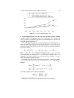
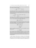
Suppose that we observe variation in market demand because of changes in dis-
posable income. Such variation in demand will trace out the pricing curve, i.e., the
optimal prices of suppliers at different quantity levels. The situation is illustrated in
figure 6.2, which shows the changes in price and quantity in a market following a
shift in demand from D
1
to D
2
. Notice in particular that demand shifts trace out the
pricing equation to give data points such as (Q
1
;P
1
) and (Q
2
;P
2
), but that such
a pricing equation is consistent with different forms of competition in the market.
First it is consistent with the firm setting P D MC in a case where marginal costs are
increasing in quantity, in which case the “pricing equation” is simply a marginal cost
310 6. Identification of Conduct

Q
P
P
1
P
2
Q
1
Q
2
MR
1
MR
2
MC
M
D
1
D
2
S = Pricing equation
Market
Market
Figure 6.2. Demand shifts do not identify conduct.
Source: Authors’ rendition of figure 1 in Bresnahan (1982).
curve. Second, the same pricing curve could be generated by a more efficient firm
that exercises market power by restricting output so that marginal revenue is equal to
marginal cost but where marginal revenue is not equal to price. If the pricing curve is
the marginal cost curve, then we are in a price-taking environment. If the firm faces a
lower marginal cost curve and is setting MR = MC and then charging a markup, the

firm has market power. The two ways of rationalizing the same observed price and
quantity data are shown in figure 6.2. The aim of the figure is to demonstrate that the
demand shift provides no power to tell the two potential underlying models apart
(unless we have additional information on the level of costs) even though demand
shifts do successfully trace out the pricing equation for us.
6.2.2.5 Identifying Conduct when Cost Information Is Not Available:
Demand Rotations
The underlying behavioral assumption in each of the three models considered is
that firms maximize profits and to do so they equate marginal revenue and marginal
costs. Each of the three models (competitive, Cournot, and monopoly) differs only
because they suggest a different calculation of marginal revenue and this has direct
implications for the determinants of the pricing curve. Each model places a differen-
tial importance on the slope of (inverse) demand for the pricing equation. This can
be seen directly from the first term in the first-order condition which describes the
pricing equation, QP
0
.Q/CP.Q/ D MC.Q/.Alternatively, we can rearrange this
equation to emphasize that prices are marginal cost plus a markup which depends
6.2. Directly Identifying the Nature of Competition 311
MC
M
D
2
MR
2
Q
P
MR
3
D

3
E
2
MC
C
E
1
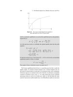
Figure 6.3. Reactions of competitive firm and monopolist to a demand rotation.
Source: Authors’ rendition of figure 2 in Bresnahan (1982).
on the slope of demand, P.Q/ D MC.Q/ C QjP
0
.Q/j, differentially across the
models.
This equation suggests a route toward achieving identification. Specifically, if
a variable affects the slope of demand, then each of the three models will make
very different predictions for what should happen to prices at any given marginal
cost. For the clearest example, note that in the competitive case absolutely nothing
should happen to markups while a monopolist will take advantage of any decrease in
demand elasticity to increase prices. Given this intuition, we next consider whether
conduct can be identified when the demand curve rotates.
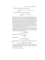
Rotation of the demand curve changes the marginal revenue of oligopolistic firms.
Flatter demand and marginal revenue curves will cause firms with market power
to lower their prices. On the other hand, price-taking firms will keep the price
unchanged since lowering the price would cause them to price below marginal cost
and make losses. Figure 6.3 illustrates this point graphically by considering a demand
rotation around the initial equilibrium point, E
1
. In particular the figure allows us to
compare the lack of reaction of a price-taking firm, which starts and finishes with
prices and quantities described by E

1
, with the response of the monopolist who
begins at E
1
but finishes with different price and quantities, those at E
2
, after the
demand rotation.
Intuitively, demand rotations allow us to identify conduct even when we have
no information about costs because such changes should not cause any response in
a perfectly competitive environment, there should be some response in a Cournot
market and a much larger response in a fully collusive environment. If demand
312 6. Identification of Conduct
becomes more elastic, prices willdecrease and quantity will increase in a market with
a high degree of market power. If, on the other hand, demand becomes more inelastic
and consumers are less willing to adjust their quantities consumed in response to
changes in prices, then prices will increase in oligopolistic or cartelized markets.
Prices will remain unchanged in both scenarios if the market is perfectly competitive
and firms are pricing close to their marginal costs.
While intuitive, a simple graph cannot show that given an arbitrarily large amount
of data a demand rotator is sufficient to tell apart the three models, which is the
statement that we would like to establish for identification. We therefore examine
the algebra of demand rotations.
Let us look at the algebra of identification using the demand rotation. Formally, we
can specify a demand function to include a set of variables Z that will affect the
slope (and potentially the level) of demand:
Q
t
D ˛
0

C ˛
1
P
t
C ˛
2
X
t
C ˛
3
P
t
Z
t
C ˛
4
Z
t
C u
D
1t
:
For our three models the encompassing pricing equation becomes
P
t
D
Â

˛
1

C ˛
3
Z
t
Ã
Q
t
C ˇ
0
C ˇ
1
Q
t
C ˇ
2
W
t
C u
S
2t
:
To consider identification note that if we can estimate demand and retrieve the true
parameters ˛
1
and ˛
3
, then we can construct the variable Q

DQ=.˛
1

C ˛
3
Z/.
In that case, the conduct parameter will be the coefficient of Q

when estimating
the following equation:
P
t
D ˇ
0
C Q

t
C ˇ
1
Q
t
C ˇ
2
W
t
C u
S
2t
:
An important challenge in the demand rotation methodology is to identify a situa-
tion where we can be confident that we have a variable which resulted in a change in
the sensitivity of demand to prices. On the other hand, a nice feature of the demand
estimation method is that when estimating the demand curve we can test whether a

variable actually does rotate the demand curve or whether it merely shifts the curve.
Events that may change the price elasticity of a product at a particular price include
the appearance of a new substitute for a good or a change in the price of the main
substitutes. For instance, the popularization of the downloading of music through
the internet may have increased the elasticity of the demand for physical CD play-
ers because consumers may have become more price sensitive and more willing to
decrease their purchases of music CDs in the case of a price increase. In the case
of digital music, one might expect that there has been both a demand rotation and
a demand shift so that at given prices, the demand for physical CDs has dropped.
Only the demand rotation will help us identify conduct. Similarly, weather may
affect both the level of demand for umbrellas and also demand may be less elastic
6.2. Directly Identifying the Nature of Competition 313
when it is raining. While there is no theoretical difficulty if the same variable affects
both the level and the slope of demand, we may run into the practical difficulties
associated with multicollinearity, which may make telling apart the demand shift
and the demand rotation rather hard empirically. Empirical work is challenging and
also requires creativity.
A second important practical issue is the difficulty of explaining a somewhat
technical issue to a nontechnical legal audience. However, this can be overcome by
understanding the principles and explaining them correctly in plain language. By
using demand rotators, we are trying to use the fact that firms with market power
will adjust to changes in the level of their market power while firms with no market
power will price close to marginal cost and will not react to changes in the level of
demand elasticities. Firms pricing close to marginal cost will not react to changes
in the price sensitivity of demand while firms with some degree of market power
will adjust their prices to such changes, according to these models.
A third issue is whether to estimate  or test models with particular values against
one another. If we estimate , we will rarely (or never) get values of 0 or 1 but
most likely something between the two. In practice, we would get an estimate of,
say,  D 0:234 352 and we could then test the hypotheses that  D 0 or  D 1 or

 D 1=N , where N is the number of firms, since we know that these correspond to
competition, perfect collusion, and the Cournot model. For example, we could test
whether the data suggest that the parameter value is more likely to be one or another
value of the parameters using, for example, a likelihood ratio test (see, in particular,
Vuong 1989). Such an approach allows us to tell whether the data are consistent
with one of the three models given enough data.
The reason to prefer the specific values of  is that we are usually really trying
to test which of the three specific models best fit the data since it can be difficult
to draw a specific conclusion on a value of  between 0 and 1 that does not equal
any of the values predicted by the theory models we have outlined. Specifically, we
do not usually have a model which corresponds directly to an estimated value of a
number like  D 0:234 352. For that reason most researchers prefer to test between
the perfect competition, the perfect cartel model, and the symmetric Cournot model
rather than over-interpreting intermediate values of . That said, in a challenge to
that practice, Kalai and Stanford (1985) do present a model which may rational-
ize a continuum of equilibrium solutions between the competitive and monopoly
outcomes.
Finally, we note the difficulties researchers face when identifying marginal costs
using first-order conditions derived from theoretical models, particularly when the
theoretical model involves some level of market power. The estimation approach
we described implies that a researcher is able to identify both demand and supply
equations, and subsequently marginal costs. There are some mixed assessments of
our ability to identify marginal costs using first-order conditions derived from theory.
Genovese and Mullin (1998) test this methodology by comparing costs implied by
314 6. Identification of Conduct
the estimated conduct and demand structure with the actual cost data in the cane
sugar refining industry in the late nineteenth century and early twentieth century
in the United States. They first find that the estimated conduct parameter using no
cost data is not too different from the one derived using actual cost information. The
estimated costs will nevertheless be very sensitive to the imposition of a particular

static model of competition. The authors defend the usefulness of defining a “loose”
conduct parameter in the specification of the pricing equation. Corts (1999) and
Kim and Knittel (2006) have less enthusiastic assessments of the accuracy of the
estimated costs when a particular competitive setting is imposed. The estimated
marginal costs, those consistent with the estimated demand elasticities and price
levels, will sometimes be negative. The reason is clear: if demand is estimated to be
inelastic but observed prices are actually fairly low, then margins can be predicted to
be so high that the only marginal costs that can rationalize the high margins would
be negative. In a recent paper Kim and Knittel (2006) find that the conduct parameter
technique poorly estimates markups and markup adjustments to cost shocks in the
California electricity market.
Corts argues that the estimation of conduct parameters in the above methodology
will often fail to measure market power accurately not least because the model of
perfect collusion Bresnahan emphasizes is not motivated from a specific dynamic
pricing model of collusion and moreover it is only one of many potential models of
collusion (other models of collusion may have features such as price rigidity making
such exercises likely to be problematic). Salvo (2007) argues that unobserved con-
straints faced by firms can limit their pricing levels resulting in an underestimation
of their ability to react to price changes following changes in demand conditions.
Concretely, he shows that threat of entry kept the prices of a cement industry cartel
in Brazil lower than would have been predicted by its documented market power.
The conduct parameter technique miscalculates the costs and underestimates the
degree of market power in that particular case. On the other hand, Salvo provides
a potential solution to the threat of entry difficulty while Puller (2006) and Kim
(2005) each suggest a solution to at least one element of the Corts critique.
In summary, the objective of this branch of the industrial organization literature
is to facilitate our ability to test between the various models of firm behavior to see
which best matches the data. In order to test one model against the other we must have
some appropriate sources of identifying data variation. In the case we examined the
sources of the required data variation were isolated as (1) demand shifters, (2) cost

shifters, and (3) demand rotator(s). In all but very special circumstances all three
were required.
More generally, the main theoretical and practical challenge to such an approach
is to understand the kind of data variation that will help distinguish one economic
model from another and then find an actual variable or set of variables which provide
that source of data variation in the particular case at hand. While the homogeneous
product Bertrand, Cournot, and perfect collusion cases studied by Bresnahan are
6.2. Directly Identifying the Nature of Competition 315
now well-understood, the challenge to develop a raft of identification results for
standard industrial organization models has not been widely taken up by the indus-
trial organization academic community and there are numerous important exam-
ples of identification results which remain to be explored and tested. For example,
one case that regulators and competition authorities should certainly like to under-
stand would involve identification results for the difference between Ramsey and
monopoly prices. Identification results exist for only a relatively small subset of stan-
dard industrial organization models.
26
For that reason a major and important topic
for future research in industrial organization involves the study of identification.
6.2.3 Identifying Tacit Collusion
Collusion occurs when firms in an industry coordinate to maximize (or at least
increase) joint industry profits as opposed to individual profits. In standard models
of oligopolistic competition, firms maximize their own profits and ignore the conse-
quence of their actions on competitor’s profitability. As a result of this fundamental
horizontal externality, whereby a firm takes actions (e.g., increases output or cuts
prices) without any consideration of the negative impact on its competitors’ profits,
total industry profits are not maximized and firms will end up producing more and at
lower prices than if they were acting together in a concerted fashion. Thus economic
theory argues that selfish actions by individual firms are (i) ultimately self-defeating
and (ii) ultimately generate great benefits for consumers in the form of lower prices

and higher output.
In any discussion of collusion, it is useful to distinguish between a cartel or explicit
collusion and tacit collusion. In an explicit cartel, firms will directly communicate
with each other about their expected behavior and reactions and will jointly decide
on the market outcome.
27
In contrast, under tacit collusion, there will be no explicit
communication, but firms will nonetheless understand their rivals’ likely reactions
when setting output and prices. If a sufficiently large fraction of the players in
an industry understand that selfish behavior will ultimately be self-defeating and
they also understand that their rivals understand that, we may find that coordinated
behavior emerges even without the need for explicit communication. Under such
tacit collusion, the expected reaction of competitors to moves in prices or output
26
One area where this line of research—the development of identification results—has been more
active is the auction literature (see, for example, Athey and Haile 2002).
27
For an extensive discussion of the determinants of the success of cartels, see the edited volume by
Grossman (2004). For a detailed discussion of three prominent U.S. cases during the 1990s (the lysine,
vitamins, and citric acid cartels), see the account by Connor (2001). The title comes from an infamous
quote by James Randall, President ofArcher-Daniels-Midland of the United States during a meeting with
fellow lysine cartel members Anjinimoto Co. of Japan in 1993. Mr. Randall was captured secretly on
tape by another ADM employee (who had signed an agreement with the FBI to be an informant in their
investigation). A fuller version reads (see Eichenwald 1997, 1998): “We have a saying at this company,”
said Mr. Randall. “Our competitors are our friends and our customers are our enemies.”
316 6. Identification of Conduct
will be to follow these moves. Firms may succeed in tacitly coordinating using sig-
naling of strategies through media, suppliers, or customers and perhaps also engage
in occasional punishments so that, without needing explicit communication, firms
end up pricing in ways that increases margins and total industry profits. Informal

evidence of both tacit and explicit collusion can emerge from company pricing or
strategy documents.
Legally, the treatment of the two forms of collusion is radically different as cartels
are per se illegal and even criminalized in many jurisdictions (including the United
States, the United Kingdom, Israel, Korea, and Australia) while tacit collusion is
not typically criminalized and yet would, at least in principle, be subject to antitrust
enforcement. For example, in the European Union, some forms of tacit collusion
could be covered by Article 81, which prohibits “concerted practices.” In addition,
tacit collusion would be included in the concept of “collective dominance,” which
has been interpreted by the courts as a particular form of “dominance” and abuse
of dominance is, for example, prohibited under Article 82.
28
In addition, mergers
that are thought to result in an increase of “collective dominance” are forbidden in
EU law. Furthermore, sector inquiries (in the EU) and in particular market inquiries
(in the United Kingdom) can be used to target industries where such behavior is
suspected.
The legal distinctions between tacit and explicit collusion may reflect economic
reality since explicit and tacit collusion differ in the sense that the form and nature
of collusion are typically explicitly agreed between the players in a cartel, so that
it may be more effective at raising prices or restricting output than a collection of
firms that are only tacitly colluding. Specifically, tacit colluders must find ways
to convey sufficient information to each other indirectly, and they must overcome
uncertainty about the extent to which rivals are “playing along” since the kind
of direct—perhaps face-to-face or even evidenced with independent accounting
reviews—reassurance possible in a cartel will not generally be possible for tacit
colluders. Such communication difficulties may diminish either the effectiveness of
the collusive arrangement or its longevity. The lack of direct communication may in
particular reduce a tacitly colluding set of firms’ability to react optimally to changes
in market conditions.

Both cartels and tacitly collusive accommodations can be unstable. Successful
coordinated behavior will generate high prices, high margins, and low output and
28
See, in particular, Laurent Piau v. Commission T-193/02, which confirms that collective dominance
can be a form of dominance for Article 82, a view already existent in the EC merger regime following
Airtours. On the other hand, a tacit collusion case has not arisen yet and indeed it would be an unusu-
ally difficult case since it would simultaneously be both a (i) “collective dominance” case and (ii) an
“exploitative abuse” case (i.e., prices are high). Each form of case is rare. Specifically, Laurent Piau v.
Commission involved a football industry association, FIFA, which introduced structural links between
companies, whereas a tacit collusion case would not involve direct linkages. Furthermore, exploitative
abuse cases against (single) dominant firms are rare in comparison to “exclusionary abuse” cases such
as those involving predatory pricing. Thus it seems a pure tacit collusion case could in principle now be
developed, but would need to overcome two potentially very difficult hurdles.
6.2. Directly Identifying the Nature of Competition 317
as a result every firm will have a private short-run incentive to increase its sales to
take advantage of the higher margin. But it must do so undetected so that there are
no reactions by competitors to eliminate the benefits of the deviation. If competitors
respond by increasing their own output and causing prices to drop to competitive
levels, the benefits of the deviation and thereby the incentives to deviate disappear.
The potential lack of stability of a collusive agreement is therefore related to the
likelihood that firms can carry out deviations that are both significant and undetected
or a detectable deviation that brings enough profits to more than compensate for the
losses of the cartel benefits. On the other hand, game theorists since the 1970s
have demonstrated that there do exist credible punishment mechanisms that can
eliminate incentives to deviate from a collusive agreement and result in stable tacitly
collusive equilibria.
29
Furthermore, some “stable” agreements are of rather complex
appearance. For example, some will involve recurrent periods of apparent “price
wars” but in fact these are just one part of the stable agreement designed to deal

with episodic periods of low demand resulting in low prices (Green and Porter 1984).
Either form of collusion in an industry harms consumers because it drives market
prices up (and output down) toward monopoly outcomes where firms can extract
much of the value generated by market activity to the detriment of consumers. It is,
however, difficult to detect collusion when evidence of explicit collusion is missing
or does not exist. How do we identify cartelized behavior from price competition?
How do we distinguish tacit collusion from legitimate oligopolistic competition?
6.2.3.1 Difficulties in Directly Identifying Tacit Collusion
Identifying tacit collusion or the likelihood of tacit collusion is notoriously difficult.
One direct approach to showing the existence of collective dominance is to attempt to
establish the extent to which any firm’s price is based on market demand sensitivity
to price changes as distinct from the firm’s own demand sensitivity to price changes.
To understand the logic of this direct approach, consider first that an indication
from company documents that a firm’s prices are being set with the reaction of
consumers in mind is an indication of market power (although every firm has some
degree of market power and not every firm is involved in pricing behavior of concern
to competition authorities). If the prices of an individual firm are found to be set
taking into account the anticipated full extent of the reaction of market demand
as distinct from their own firm’s demand, then we may have an indication of a
collusive industry. Indeed, on the face of it, if the firm monitors and takes into
account the effect of its actions on other market participants profitability, then we
potentially have direct evidence for tacit or explicit collusion. In practice, such
evidence must be interpreted carefully as many firms will engage in monitoring
of rivals’ behavior and this may be normal strategic behavior as distinct from the
kind of dynamic strategic behavior that results in collusive outcomes. Evidence of
29
This is formalized in Friedman (1971) and Abreu (1986).
318 6. Identification of Conduct
monitoring rivals is certainly not in itself evidence of tacit collusion. Rather we
must find evidence that the firm is taking, or attempting to take, decisions which

actively accommodate its rivals’ needs and in particular their likely profitability.
Such direct evidence may be available from company documents or testimony,
but even apparently direct documentary evidence can appear ambiguous given the
intervention of skilled legal professionals. Evidence may also be available from
econometric analysis (following the approach to identifying collusion outlined in
the first part of this chapter which emphasized the power of “demand rotators” for
identification in simple models) but again such evidence is rarely unambiguous. The
difficulty in making these distinctions in practice should not be understated.
To further understand the difficulties in establishing tacit collusion directly, note
that firms may tacitly collude with varying degrees of success. First, if firms are
heterogeneous, they may not gain much directly from the optimal tacitly collusive
action. For example, consider that a two-plant monopolist may sometimes minimize
costs by using only its most efficient plant and not its inefficient plant. A tacitly collu-
sive arrangement between two single-plant firms in which one firm produced nothing
would probably be difficult to sell to the owner of the unused plant, at least without
some form of (possibly indirect) side-payments between players, perhaps through
industry associations, shared industry-level advertising, or commercial activities in
other markets. Second, the world changes and tacitly colluding firms must have a
strategy for dealing with change. For example, demand or costs may be high or low
and, in a standard model of firm behavior, collusive prices would change with costs
and demand conditions. If so, then tacitly colluding firms may need to re-establish a
new tacit agreement about the level of collusive prices fairly frequently. However, if
change threatens stability, then collusive arrangements may well involve only very
infrequent changes in pricing or market territories. For each of these reasons the
outcomes of a tacitly collusive arrangement can be somewhat or greatly distinct
from either competitive or perfectly collusive outcomes.
We have already mentioned the critique of the econometric attempts to measure
market power provided in Corts (1999). However, the critique in large part also
applies to noneconometric evidence. Fundamentally, the problem is that dynamic
game theory has only succeeded in showing that tacit collusion may be a sustainable

market outcome and then provided us with a wide variety of examples of (potentially
complex) pricing strategies that could result. The theory has not then yet provided a
comprehensive “identification” strategy for distinguishing general classes of mod-
els of collusion from models of competition. Numerous market histories appear
consistent with collusion and yet also appear consistent with other competitive
environments. For example, collusion can produce stable prices or a succession of
price wars depending on the level of uncertainty or the nature of the punishments.
Collusion may also produce procyclical or countercyclical prices depending on, for
example, capacity utilization levels or whether we are at turning points of business
6.2. Directly Identifying the Nature of Competition 319
cycles or not.
30
Some consensus has emerged on the conditions that are more likely
to promote collusion: small numbers of players, stability of demand, and firm sym-
metry.
31
But these characteristics are mostly indicative as collusion is still possible
when these characteristics are absent. For example, symmetry will rarely be the case
in differentiated product markets and, we shall see, firm asymmetry makes collusion
harder in at least one important sense, but on the other hand does not typically rule
out situations arising when collusion can nonetheless be sustained.
Because of the apparently weak predictive power of economic theory with regards
to the exact manifestation of collusion, most empirical casework to detect collusion
has centered on showing that the very basic conditions that are necessary for collu-
sion to exist can be found in a givenmarket. The presumption is that if these necessary
conditions exist (so that firms have both the ability and incentive to collude), then
collusion is likely. The analysis of coordination in antitrust settings currently tends
to consist of analysis of the three essential points introduced by Stigler (1964) nearly
fifty years ago, which we present below.
6.2.3.2 Assessing the Conditions for Agreement, Monitoring, and Enforcement

Stigler (1964) provided a general framework for evaluating the features of a mar-
ket which are likely to facilitate the movement toward coordination. Subsequently
this framework has largely been adopted in most jurisdictions, although the exact
terminology varies from guidance to guidance.
32
It relies on the conclusion that for
collusion to be viable, it must be feasible for participants to reach an agreement on
the terms of coordination; it must also be possible to monitor that this agreement is
being respected by the colluding firms; and deviating firms must be punished and,
in the case of tacit collusion, it is the credibility of this punishment mechanism that
holds the collusive agreement together, i.e., enforces it. The framework is equally
applicable for explicit or tacit collusion, but the form of each element can differ. In
the case of cartels for example, agreement may be arrived at by discussion, moni-
toring may occur by exchange of information, perhaps even independent reports by
accounting firms and/or trade associations, while enforcement may in some cases
remain via similar mechanisms to those emerging from tacit collusion.
33
In others
the mechanism may be quite different. For example, in the extreme case of legal
cartels, enforcement may result from contract enforcement via the courts. It is worth
noting that export cartels remain legal in a number of jurisdictions. We next discuss
each element of Stigler’s framework in turn.
30
See, in particular, Rotemberg and Saloner (1986) and Haltiwanger and Harrington (1991). See also
Garc´es et al. (2009) for a brief review of the subsequent collusion literature.
31
For a summary of the literature, see Ivaldi et al. (2003).
32
For example, the categories Agreement, Monitoring, and Enforcement are sometimes replaced with
the terms Consensus, Detection, and Punishment.

33
For example, in the lysine case, sales were reported to a trade association and each year a firm of
accountants audited the sales numbers in both London and Decatur, IL.
320 6. Identification of Conduct
Agreement. Colluders must reach some form of understanding about what exactly
it means to coordinate. This means that there must be an understanding of the
dimensions on which coordination is taking place as well as an indication of the
expected behavior. In tacit collusion the agreement will not be explicit but will have
to be inferred by market players from the information available to them. Firms can
publicize their price lists and make public announcements to provide the market with
an indication of a potential focal point around which behavior will be coordinated.
These signaling practices are normally frowned upon by market authorities when
they suspect collusive behavior, but on the other hand publishing price information
is not uncommon and in other circumstances is actively encouraged by competition
authorities, for example, to facilitate consumer search. Focal points may also be
inferred from past behavior or historical prices and in such cases markets may tend
to exhibit stronger degrees of price rigidity. A market with complex transactions or
with customized transactions will be less susceptible to firms being able to find a
mutually acceptable understanding of what it means to tacitly collude. Similarly, a
market with very diverse products such as different brands and different versions of
a particular product will be more difficult to coordinate. Since complexity makes
agreements about what it would mean to collude difficult to achieve, sometimes we
see firms adopting practices that “simplify their prices for consumers” or harmonize
the conditions for a transaction. For an example of a pricing structure which might
be considered by some authorities to potentially facilitate collusion, recall that at
one stage some U.S. airlines proposed using per-mile pricing so that every route
between every city would be easy to price by all parties.
34
Such initiatives may have
the ultimate purpose of facilitating a collusive outcome since coordination largely

reduces to tacitly agreeing on a single number, the per-mile price. Finally, when firms
have very different incentives, perhaps because of differences in scale or efficiency,
it will be harder to get everyone to agree to a particular market outcome. It may be
easier to evolve toward agreements in industries where change occurs only slowly as
it is not always obvious for firms to understand or agree on a coordinated response
to change.
In a coordinated effects merger case it is desirable but probably should not be
necessary to say exactly what the form of a coordinated agreement might look like,
since it is unlikely that a competition authority will put the same effort into find-
ing an ingenious solution to a difficult problem as the companies involved, should
they have a sufficiently strong incentive to cooperate. For this reason, most com-
petition authorities do not give quite the same weight to the agreement element of
Stigler’s framework in their guidelines as they do to the monitoring and enforce-
ment areas. Even explicit agreements can be incredibly difficult to uncover. In the
famous “phases of the moon” cartel case, twenty-nine colluding firms in the market
34
See, for example, O’Brian (1992). To see that such proposals may not succeed, see, for example,
McDowell (1992).
6.2. Directly Identifying the Nature of Competition 321
for electrical equipment led by the two giants General Electric and Westinghouse
literally devised a codebook of lists of numbers which determined how much each
company in the cartel would bid on a particular contract. The price spread was geared
toward giving an impression of competition and the fact that the price spreads across
companies were cyclical led to the cartel being known as the “phases of the moon”
cartel. That particular cartel lasted seven years and rigged bids estimated to be worth
a total of $7 billion.
35
Monitoring. Dynamic oligopoly theory suggests that for coordination firms must
be aware of the behavior of their competitors. They must be able to observe it
or at least to infer it with certain degree of confidence. In particular they must

be able to spot deviations from prevailing behavior in order that “cheaters” from
the coordinated prices can be spotted. Monitoring will be harder in markets where
prices and/or quantity choices are difficult to observe, demand or cost shocks are
large, or when orders are lumpy and as a result both prices and quantities tend to
be volatile. But it has been argued in the economics literature that tacit collusion
can certainly occur without full transparency. Specifically, the literature emanating
from Green and Porter (1984) has shown that tacit collusion is possible even without
full monitoring of firms’ prices and quantities. For example, a strategy that would
temporarily revert to a price war every time market prices fell below a threshold
can sustain tacit collusion.
36
In this case, tacit collusion would take the form of
alternating phases of price stability and price wars.
In spite of these contributions, the issues of transparency, complexity, and the abil-
ity to monitor competitors’actions and prices are usually considered very important
for a finding of collusion or coordinated effects. It is possible to look at the extent of
monitoring and the extent of both complexity and transparency of information both
through interview evidence and documentary evidence. Price lists, price announce-
ments, and industry association publications are clear ways of announcing one’s
behavior but more may be needed to detect small-scale deviations. List prices or
“price books” can sometimes facilitate coordination because they can dramatically
improve the amount of information available to rivals. If customers mainly pay list
prices, or list prices are highly correlated with transaction prices (in the extreme,
transaction prices may be some fixed discount from list prices), then such price lists
may help firms find their way toward coordination. Price lists need not be paper
price lists and in some famous examples the price lists have been electronic. For
example, in the U.S. Airline Tariff Pricing case, participating U.S. airlines could
post nonbinding ticket prices for particular routes that were for an initial period
unavailable to customers. In fact, they used features of the electronic fare system
35

For a wonderful description of what has become known as the great electrical conspiracy, see “The
great conspiracy,” Time Magazine, February 17, 1961.
36
For the first test of the Green and Porter model, see Porter (1983).
322 6. Identification of Conduct
84
89
94
99
104
109
114
119
124
311357911131517192123252729
Period
List prices
Figure 6.4. List prices versus actual prices.
Source: Scheffman and Coleman (2003, figure 4).
as signaling devices.
37
Baker (1996) provides an interesting commentary on infor-
mation exchange in cyberspace. However, before condemning price lists, one must
keep in mind that, at their best, price lists can hugely improve the information avail-
able to consumers which in turn can save consumer search costs, increase the price
sensitivity of demand, and encourage firms to charge lower prices than their rivals.
Information flows between customers and suppliers in the case of stable customer–
supplier relationships can be an important way of getting exact market information
particularly when customers shop from different suppliers. The visibility of contracts
and of changes in market shares is useful to detect potential deviations. Investiga-

tors should certainly invest in assessing the level of transparency and monitoring
mechanisms that may imply that a coordinated outcome is viable.
Scheffman and Coleman (2003) provide a nice summary of the kinds of empirical
work that may be undertaken to assess coordination. Those authors emphasize that
coordination can happen in a number of ways and may involve coordination on
prices, quantities, capacities, or some form of market division, say, by territory
or type of customer. As a result many of the following remarks while phrased in
terms of prices are equally relevant to other potential dimensions of coordination.
Scheffman and Coleman suggest, for example, that we may wish to look empirically
at the following:
1. Differences or patterns in the relationship between list and transaction prices.
Figure 6.4 provides an example where list prices have little predictive power
for actual transaction prices. In this case, list prices do not carry enough infor-
mation about actual market prices and cannot be used as a monitoring device.
37
United Stated v. Airline Tariff Publishing Co. (D.D.C., August 10, 1994) (final consent decree).
6.2. Directly Identifying the Nature of Competition 323
Table 6.5. Example of a company’s estimates of competitor activity
Competitor Y Competitor Z
Number of customers that company X
identifies as supplying 55 46
identifies as supplying when did not 22 12
does not identify as supplying when did 12 8
Percentage of customers for whom company X’s
volume estimate was off by more than 20% 75% 82%
volume estimate was off by more than 60% 39% 47%
Source: Scheffman and Coleman (2003, figure 5).
2. Variation in prices across consumers, controlling for observable differences
in the type of customer or order behavior in terms of volume or location. We
can look at the coefficient of variation and range of prices paid by various

customer types. To that end a transaction-level regression of price on volume,
location, and customer characteristics may be run in order to understand and
evaluate the extent of variation in prices across customers or customer groups.
3. Variation in transaction prices within customer for the same product across
different suppliers. We may also want to look at the percentage of instances
where prices to the same customer by different suppliers differ by, say, more
than 5%. We might, for example, want to break that down by customer type.
4. Variation in changes in transaction prices across customers again controlling
for observable differences.
As with all such studies it is vital to bear in mind that the mere existence of co-
movement in, say, list and transaction prices does not prove coordination since
we would expect co-movement to result for innocent reasons such as cost variation.
However, the basic intuition that such analysis relies on is that if significant variation
in a firm’s price changes is found, we might expect that coordinated interaction is
likely to be more difficult. We examine this approach further (see section 6.2.3.4)
by looking at the European Commission’s empirical evidence in the Sony–BMG
merger case.
We may also want to look at transparency directly by comparing one company’s
estimates of competitors’ volumes versus their competitors’ actual volumes. Such
an analysis is provided in table 6.5, which shows that competitor X’s estimates were
quite considerably different from the truth.
Enforcement. In the theory of tacit collusion, enforcement action involving mem-
bers of the cartel (internal enforcement) takes the form of the threat of a credible
punishment directed at either a deviating firm or in a nontargeted fashion at all firms
if they move away from the tacitly collusive outcome when a deviation is detected.
324 6. Identification of Conduct
A successful punishment regime will eliminate the potential gains from cheating
on other participants. When cheating on a collusive agreement is easily detected
and a credible punishment exists for such behavior, tacitly collusive environments
are predicted to be stable. Moreover, in some (at least theoretical) environments, no

actual punishments need ever be observed which may make detection by competition
authorities rather difficult.
On the other hand, while many theoretical models generate tacit collusion rather
easily,itdoesseemthateven explicit cartels, where direct communication is possible,
do certainly break down. In a review of a large set of known cartels, Suslow and
Levenstein (1997) find that the average longevity of an explicit cartel is about five
years but that the distribution is bimodal: while some cartels last for decades, many
others last for less than a year.
In addition to a mechanism that enforces internal stability of a collusive arrange-
ment, there must be some form of mechanism for enforcing “external” stability. In
particular, all else equal, high profits will soon attract new entrants so that it will
be necessary to have either actual barriers to entry or an ability to punish entrants
so as to deny them returns (in the sense of profit) following entry. For example,
in the lysine case, a cartel member, Archer-Daniels-Midland, quickly built a new
plant as part of strategy to deter a new entrant (Connor 2001). For tacit collusion to
be an antitrust problem an industry must be able to benefit from both internal and
externality stability.
In addition to suggesting that a credible punishment mechanism is important, eco-
nomic theory does make some suggestions regarding the nature of such punishments.
One particularly simple punishment involves the reversion to static competition. The
theory suggests that the threat of a permanent or even temporary price war can be an
effective punishment provided cartel participants are sufficiently patient and such
punishments may sometimes involve “harsher” punishments than reversion to the
competitive price.
38
Such theoretical results suggest that a key variable linked to the
effectiveness of punishment is the ability of the punishing firms to rapidly expand
output so that prices fall sharply enough to generate the losses that will deter oppor-
tunistic deviation. As a result there is an important literature on the role of excess
capacity both on the incentives to cheat and the ability to punish. Excess capacity

is generally considered to facilitate tacit coordination (see, for instance, Brock and
Scheinkman 1985; Davidson and Deneckere 1990). Highly asymmetric holdings of
capacity on the other hand probably, but not necessarily, hinder collusion (Compte
et al. 2002; Vasconcelos 2005).
Other forms of punishment can exist particularly in multiproduct markets,
although Bernheim and Whinston (1990) suggest that multimarket contact is actively
helpful to sustaining collusion in the presence of firm or market asymmetry (Bern-
heim and Whinston 1990). Such asymmetry seems likely to arise fairly generically in
38
See Abreu et al. (1990). Harsher punishments can involve prices below the competitive levels and
stability can sometimes be maintained by using harsh but fairly short punishments.
6.2. Directly Identifying the Nature of Competition 325
real world markets making multimarket contact potentially a relevant consideration.
Intuitively, under perfect firm and market symmetry, the incentive to collude and
the incentive to cheat for all firms in all markets will be identical so that multimar-
ket contact adds little. However, with firm and/or market asymmetry, the incentives
for collusion and cheating will generally differ across firms in multimarket con-
texts. Within market, firm asymmetry means that different firms must each find
collusion attractive. Multimarket contact means that incentive constraints will be
evaluated in total across markets rather than within any individual market. As a
result, punishments, for example, might be targeted to greatest effect.
Punishment mechanisms should be effective not only at deterring participating
firms in an industry from cheating (internal stability) but also at deterring potential
entrants in the market (external stability). Because it is difficult to discipline a very
large number of firms that could enter at any time in an industry, tacit collusion
will be more effective in markets that exhibit some barriers to entry. Indeed, in their
review of the case history, Suslow and Levenstein (1997) find that, while cartels do
sometimes break up occasionally because of cheating by incumbents, entry and an
ability to react to changes in market positions pose a greater problem. Relatedly,
not all firms in an industry will necessarily be involved in a particular cartel and if

customers of those which are in a cartel can react by switching to nonparticipating
suppliers, then that will help destabilize a collusive equilibrium.
While Stigler (1964) introduces the agreement, monitoring, and enforcement
framework we have described, there is an important question as to the extent of
analysis necessary about the form of the likely agreement. In particular, the summary
of the European Court of First Instance judgment in the Airtours case reads:
39
Three conditions are necessary for the creation of a collective dominant position
significantly impeding effective competition in the common market or a substantial
part of it:
– first, each member of the dominant oligopoly must have the ability to know
how the other members are behaving in order to monitor whether or not
they are adopting the common policy. In that regard, it is not enough for
each member of the dominant oligopoly to be aware that interdependent
market conduct is profitable for all of them but each member must also have a
means of knowing whether the other operators are adopting the same strategy
and whether they are maintaining it. There must, therefore, be sufficient
market transparency for all members of the dominant oligopoly to be aware,
sufficiently precisely and quickly, of the way in which the other members’
market conduct is evolving;
– second, the situation of tacit coordination must be sustainable over time, that
is to say, there must be an incentive not to depart from the common policy on
the market. It is only if all the members of the dominant oligopoly maintain
the parallel conduct that all can benefit. The notion of retaliation in respect of
conduct deviating from the common policy is thus inherent in this condition.
39
Airtours plc v. Commission of the European Communities, Case T-342/99.
326 6. Identification of Conduct
In that context, the Commission must not necessarily prove that there is a
specific retaliation mechanism involving a degree of severity, but it must none

the less establish that deterrents exist, which are such that it is not worth the
while of any member of the dominant oligopoly to depart from the common
course of conduct to the detriment of the other oligopolists. For a situation
of collective dominance to be viable, there must be adequate deterrents to
ensure that there is a long-term incentive in not departing from the common
policy, which means that each member of the dominant oligopoly must be
aware that highlycompetitive action on its part designed to increase its market
share would provoke identical action by the others, so that it would derive
no benefit from its initiative;
– third, it must also be established that the foreseeable reaction of current and
future competitors, as well as of consumers, would not jeopardise the results
expected from the common policy.
Broadly, the first condition relates directly to monitoring, while the second and third
relate directly to internal and external enforcement. Thus, the agreement element of
Stigler’s framework is played down in the current EU legal environment presumably
for reasons we have discussed earlier in this section.
In establishing these conditions, the competition case handlerwill need to examine
carefully the specific facts about an industry,understanding the nature of multimarket
contact, the extent of asymmetry, the lumpiness or orders, and so forth. An analyst
would also go on to attempt to understand at least qualitatively the incentives of
firms in an industry to sustain collusion and hence their ability to do so before she
is able to conclude whether tacit collusion is likely or unlikely to be viable.
6.2.3.3 Other Evidence Potentially Relevant to an Inference of the Presence of
Tacit Coordination
The issue of whether mergers are likely to increase the likelihood of tacit collusion
will most certainly consist of an assessment of the evidence regarding the three
elements discussed above, in particular in Europe as determined by the Court of
First Instance’s Airtours decision of 2002. Regarding the assessment of existing
tacit collusion, the Court for First Instance in its Impala judgment said that:
in the context of the assessment of the existence of a collective dominance

position, although the three conditions defined by the CFI inAirtours v. Commission
. . . are indeed also necessary, they may, however, in the appropriate circumstances,
be established indirectly on the basis of what may be a series of indicia and items
of evidence relating to the signs and manifestations and phenomena inherent in the
presence of a collective dominant position. (251 Impala v. Commission)
40
The European Court of Justice, in its annulment of the CFI decision, upheld the
right of the court to freely assess different items of evidence. It also argued against
the mechanical application of the so-called Airtours conditions detailed above but
40
Impala v. Commission of the European Communities, Case T-464/04 (2006).
6.2. Directly Identifying the Nature of Competition 327
rather asked for these criteria to be related to an “overall economic mechanism of a
hypothetical tacit coordination.”
41
So that any evidence pointing to tacit collusion
is admissible but a realistic mechanism of collusion consistent with the economic
theory of collusion must also be laid out.
This can be understood as an invitation to use available evidence to directly
identify a collusive outcome as distinct from the outcome generated by a competitive
oligopoly. We have already seen that this is very difficult to do due in part to the lack
of a wide variety of predictions that emerge from the theoretical framework for tacit
collusion. It is particularly important to keep two factors in mind. First, coordination
need not be complete in the sense of implementing the perfectly collusive outcome
in a market. Second, information need not be perfect to sustain collusion. Most
realistic scenarios of tacit collusion assume some degree of incomplete information
which may then be reflected in some inefficiency in the reaction of the coordinated
firms.
Still, one can certainly pay attention and give proper weight to such things as the
existence of facilitating practices: observed industry practices which seem to have

no other purpose than to allow information to flow or to facilitate an agreement.
For instance, K¨uhn (2001) proposes that, given the intrinsic difficulty in inferring
whether prices are the result of competitive oligopoly or of tacit collusion, it is more
desirable to focus on suppressing certain forms of communication between firms,
which do not bring efficiency and are likely to sustain a collusive equilibrium. His
paper contains a review of the experimental evidence of the positive role of com-
munication in collusion. See also the more recent experimental evidence reported
in Cooper and K¨uhn (2009).
The extent of price rigidity may be relevant to such an evaluation of tacit collu-
sion, and/or the presence of unexplained price wars in a market, where legitimate
explanations for such outcomes can potentially be excluded. If prices sometime
oscillate widely when there are no obvious demand or cost causes, competition
authorities will want to consider alternative potential explanations, one of which is
tacit collusion.
Since all actual instances of tacit collusion are likely to occur in a world of
imperfect information, it is likely that agreements will not always work smoothly
all the time. Firms will also rarely be completely symmetric and agreements, once
reached, may not satisfy the ambitions of all players robustly. Some firms will prob-
ably have more incentives than others to cheat and to do so they will be more likely
to take advantage of sudden fluctuations in demand or costs to lower prices and
sell more than their agreed share. Competitors, unable to distinguish between the
consequences of demand changes and cheating may retaliate and all this instability
may become apparent in the data. It is possible that an examination of price series
41
ECJ ruling of 10/07/08 in case C-413/06P in particular paragraphs 117–34.