Quantitative Techniques for Competition and Antitrust Analysis_11 ppt

338 6. Identification of Conduct
econometric model, but it can also be helpful when collecting other evidence in a
given case (e.g., documentary evidence). On the other hand, such an observation
may concern us since we noted earlier that on occasion cartels have often resulted
in relatively less variation in prices, perhaps because of stability concerns. As Corts
(1999) noted, a different model of collusion would have different implications for
observed collusive prices.
6.2.4.2 Identification of Pricing and Demand Equations in Differentiated Markets
In a fashion entirely analogous to the homogeneous products case, the identification
of conduct generally requires that the parameters of the demand and pricing equa-
tions are identified. Even if demand rotation can also be used to identify conduct
in differentiated industries in the same way as is done for homogeneous products,
demand does need to be estimated to confirm or validate assumptions. This presents
a challenge because a differentiated product industry has one demand curve and one
pricing function for each of the products being sold. In contrast, in the homogeneous
product case, there is only one market demand and one market supply curve that
need to be estimated. Now we will need to estimate as many demand functions as
there are products and also as many pricing equations as there are products. Iden-
tification naturally becomes more difficult in this case and some restrictions will
have to be imposed in order to make the analysis tractable. We discuss differentiated
product demand estimation extensively in chapter 9.
A general principle for identification of any linear system of equations is that the
number of parameter restrictions on each equation should be equal to, or greater
than, the number of endogenous variables included in the equation. A normalization
restriction is always imposed in the specification of any equation so in practice
the number of additional restrictions must equal or be more than the number of
endogenous variables less one.
49
This is equivalent to saying that the restrictions
must be equal to or more than the number of endogenous variables on the “right-
hand side” of any given equation. The total number of endogenous variables is also

the number of equations in the structural model. This general principle is known as
the “order condition” and is a necessary condition for identification in systems of
linear equations. It may, however, not be sufficient in some cases. Previously, we
encountered the basic supply-and-demand two-equation system, where we had two
structural equations with two endogenous variables: price and quantity. In that case
we needed the normalization restrictions and then at least one parameter restriction
for each equation for identification. We obtained the parameter restrictions from
theory: variables that shifted supply but not demand were needed in the equations
to identify the demand equation and vice versa (these exclusion restrictions are
imposed by restricting values of the parameters to zero). A more technical discussion
49
The normalization restriction is usually imposed implicitly by not placing a parameter on whichever
one of the endogenous variables is placed on the left-hand side of an equation.
6.2. Directly Identifying the Nature of Competition 339
Table 6.7. Nature of competition in the U.S. car market.
Auto % in
production Real auto quality-adjusted Sales Quantity
Year (units) price/CPI prices revenues ($) index
1953 6.13 1.01 — 14.5 86.8
1954 5.51 0.99 — 13.9 84.9
1955 7.94 0.95 2.5 18.4 117.2
1956 5.80 0.97 6.3 15.7 97.9
1957 6.12 0.98 6.1 16.2 100.0
Source: Bresnahan (1987).
of identification of demand and pricing equations in markets with differentiated
products is provided in the annex to this chapter (section 6.4), which follows Davis
(2006d).
6.2.4.3 Identification of Conduct: An Empirical Example
When conduct is unknown, we will want to assess the extent to which firms take into
account the consequences of pricing decisions on other products when they price

one particular good. In this case, one strategy is to estimate the reduced form of
the structural equations and retrieve the unknown structural parameters by using the
correspondence between reduced-form and structural parameters derived from the
general structural specification.Assuming that the demand parameters are identified
and marginal costs are constant, we will need enough demand shifters excluded from
a pricing equation to be able to identify the conduct parameters (see Nevo 1998). In
particular, we will need as many exogenous demand shifters in the demand equation
as there are products produced by the firm. Although identification of conduct is
therefore technically possible, in practice it may well be difficult to come up with a
sufficient number of exogenous demand and cost shifters.
An early and important example of an attempt to identify empirically the nature
of competition in a differentiated product market is provided by Bresnahan’s (1987)
study of the U.S. car industry in the years 1953–57. Bresnahan considers the prices
and number of cars sold in the United States during those years and attempts to
explain why in 1955 prices dropped significantly and sales rose sharply. In particular,
he tests whether this episode marks a temporary change of conduct by the firms from
a coordinated industry to a competitive one. The data that Bresnahan (1987) is trying
to explain are presented in table 6.7. The important feature of the data to notice is
that it is apparent that 1955 was an atypical year with low prices and high quantities.
Real prices fell by 5%, quantity increased by 38%, and revenues increased by 32%.
To begin to build a model we must specify demand. Bresnahan specifies demand
functions where each product’s demand depends on the two neighboring products in
340 6. Identification of Conduct
terms of quality: the immediately lower-quality and the immediately higher-quality
product. He motivates his demand equation using a particular underlying discrete
choice model of demand but ultimately his demand function takes the form,
q
i
D ı
Ä

P
j
 P
i
x
j
 x
i

P
i
 P
h
x
i
 x
h

;
where P and x stand for price and quality of the product and h, i, and j are indicators
for products of increasing quality. Quality is one dimensional in the model, but
captures effects such as horsepower, number of cylinders, and weight. Note that, all
else equal, demand is linear in the prices of the goods h, i, and j and that given a
price differential the cross-price slopes will increase with a decrease in the difference
in quality, x. In this rather restrictive demand model there is only a single parameter
to estimate, ı.
To build the pricing equations, he assumes a cost function where marginal costs
are constant in quantity produced but increasing in the quality of the products so
that x
j

> x
i
> x
h
for products j , i , and h. These assumptions imply that the whole
structure can be considered as a particular example of a model where demand is
linear in price and marginal costs are constant in output. By writing a linear-in-
parameters demand equation, where q
i
D ˛
i0
C˛
ii
p
i
C˛
ij
p
j
C˛
ih
p
h
, we can see
that for fixed values of the quality indices, x
i
, x
j
, and x
h

, the analysis of a pricing
game using Bresnahan’s demand model can be incorporated into the theoretical
structure we developed above for the linear demand model where the parameters in
the equation are in fact functions of data and a single underlying parameter. (More
precisely, we studied the linear demand model with two products above and we will
study the general model in chapter 8.) Specifically, the linear demand parameters
are of the form,
˛
ii
Dı
Â
1
x
j
 x
i
C
1
x
i
 x
h
Ã
;
˛
ij
D ı
Â
1
x

j
 x
i
Ã
;
˛
ih
D ı
Â
1
x
i
 x
h
Ã
:
Bresnahan estimates the system of equations by assuming first that there is Nash
competition so that the matrix  describes the actual ownership structure of products
(i.e., there is no collusion). Subsequently, he estimates the same model for a cartel
by setting all the elements of the  matrix to 1 so that profits are maximized for
the entire industry. He can then use a well-known model comparison test called the
Cox test to test the relative explanatory power of the two specifications.
50
Bresnahan
50
Wehave shown thatthe two modelsBresnahan writesdownare nestedwithin a single family ofmodels
so that we can follow standard testing approaches to distinguish between the models. In Bresnahan’s
case he chooses to use the Cox test, but in general economic models can be tested between formally
irrespective of whether the models are nested or nonnested (see, for example, Vuong 1989).
6.3. Conclusions 341

P
MC
P
MC
1234 5 6 1234 5 6
(a) (b)
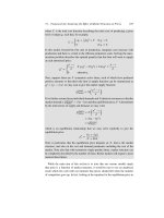
Figure 6.5. Expected outcomes under (a) competition and (b) collusion. Source: Authors’
rendition of figure 2 in Bresnahan (1987). (a) Under competition, products with close substi-
tutes produced by rivals get very low markups over MC. (b) Under collusion, close substitutes
produced by rivals get much higher markups over MC.
concludes that the cartel specification explains the years 1954 and 1956 while Nash
competition model explains the data from 1955 best. From this, he concludes that
1955 amounted to a temporary breakdown of coordination in the industry.
Intuitively, Bresnahan is testing the extent to which close substitutes are con-
straining each other. If the firm maximizes profits of the two products jointly, there
will be less competitive pressure than in the case where the firm wants to maximize
profits on one of the products only and therefore ignores the negative consequences
of lower prices on the sales of the close substitute product. Thus, in figure 6.5, if
close substitute products 2 and 3 are owned by rivals, then they will have a low
markup under competition but far higher markups under collusion.
Given his assumptions about costs and the nature of demand, Bresnahan finds
that the explanation for the drop in price during 1955 is the increase in the level of
competition of close substitutes in the car market.
The demand shifters that helped identify the parameter estimates are presented
in table 6.8 as well as the accounting profits of the industry. The accounting profits,
however, are not consistent with Bresnahan’s theory, as he notes. If firms are coor-
dinating in the years 1954 and 1956, industry profits should be higher than in 1955
when they revert to competition. Bresnahan’s response is that accounting profits are
not representative of economic profits and are not to be relied upon. We must there-
fore make a decision in this case about whether to believe the accounting measures

of profitability or the econometric analysis. In other cases, one might hope each type
of evidence allows us to build toward a coherent single story.
6.3 Conclusions
 Structural indicators such as market shares and concentration levels are still
commonly used for a first assessment of industry conduct and performance,
342 6. Identification of Conduct
Table 6.8. Demand and cost shifters of the car market in the United States 1953–57.
Per capita
disposable income Durable
‚
…„ ƒ
Interest expenditures Accounting
Year Level Growth rates (nonauto) profits ($)
1953 1,623 — 1.9 14.5 2.58
1954 1,609 0.9% 0.9 14.5 2.25
1955 1,659 3.0% 1.7 16.1 3.91
1956 1,717 3.5% 2.6 17.1 2.21
1957 1,732 0.9% 3.2 17.0 2.38
Source: Bresnahan (1987).
although they are not usually determinative in a regime applying an effects-
based analysis of a competition question. The fact that they are not determi-
native does not mean market shares are irrelevant, however, for a competition
assessment and many authors consider they should carry some evidential
weight.
 Developments in static economic theory and the availability of data have
shown that causality between market concentration and industry profitability
cannot be easily inferred. However, economic theories built on dynamic mod-
els do frequently have a flavor of considerable commonality with the older
SCP literature. For example, Sutton (1991, 1998) emphasizes that prices are
indeed expected to be a function of market structure in two-stage games where

entry decisions are made at the first stage and then active firms compete in
some way (on prices or quantities) or collude at a second stage.
 The broad lesson of game theory is that quite detailed elements of the com-
petitive environment can matter for a substantial competition analysis. The
general approach of undertaking a detailed market analysis aims at directly
identifying the nature of competition on the ground and therefore the likely
effects of any merger or alleged anticompetitive behavior.
 Technically, the question of identification involves asking the question of
whether two models of behavior can be told apart from one another on the
basis of data. The hard question in identification is to establish exactly which
data variation will be helpful in moving us to a position where we are able to
tell apart some of our various models. The academic analysis of identification
tends to take place within the context of econometric models, but the lessons of
such exercises typically move directly across to inform the kinds of evidence
that competition authorities should look for more generally such as evidence
from company documents.
6.4. Annex: Identification of Conduct in Differentiated Markets 343
 The degree to which firms are reactive to changes in demand conditions in
the market can provide direct evidence of the extent of a firm’s market power.
Formal econometric models can use the methods involving the estimation
of conduct parameters in structural models to determine whether the reac-
tions of firms to changes in prices are consistent with competitive, competing
oligopoly, or collusive settings. However, the more general lesson is that
changes in the demand elasticity can provide useful data variation to identify
conduct. For example, we might (at least conceivably) find documentary evi-
dence suggesting that firms’ pricing reactions accommodate prices in a fash-
ion consistent with a firm’s internal estimates of market demand sensitivities
(rather than firm demand sensitivities).
 We examined identification results for both homogeneous product markets and
also subsequently differentiated products markets. Analysis of identification

in the former case suggests that demand rotators are the key to identifica-
tion. In the differentiated product case, the results suggest that (i) examining
the markups of close-substitute but competing products may be useful and
(ii) examining the intensity with which demand and cost shocks to neighboring
products are accommodated may sometimes be helpful when understanding
the extent of coordination in a market.
 In examining the likelihood of collusion, one must assess whether the neces-
sary conditions for collusion exist. Following Stigler (1964), those are agree-
ment, monitoring, and enforcement. The assessment of each of these con-
ditions will typically involve a considerable amount of qualitative evidence
although a considerable amount of quantitative evidence can be brought to
bear to answer subquestions within each of the three conditions. For exam-
ple, the European Commission examined the extent to which transaction
prices were predictable given list prices to examine market transparency in
the Sony–BMG case.
 In addition to qualitative analysis of the factors which can affect the likelihood
of collusion, it is sometimes possible and certainly desirable to develop an
understanding of the incentives to compete, collude, and also to defect from
collusive environments.
6.4 Annex: Identification of Conduct in Differentiated Markets
In this annex we follow Davis (2006d), who provides a technical discussion of
identification of (i) pricing and demand equations in differentiated product markets
and (ii) firm conduct in such markets. In particular, we specify in more detail our
example of a market with two firms and two differentiated products. Define the
344 6. Identification of Conduct
marginal costs of production which depend on variables w such as input costs to be
independent of output so that
"
c
1t

c
2t
#
D
"

0
1
0
0
0
2
#"
w
1
t
w
2
t
#
C
"
u
1t
u
2t
#
:
Similarly, suppose that demand shifters depend on some variables x such as income
or population size which affect the level of demand for each of the products:

"
˛
01t
˛
02t
#
D
"
ˇ
0
1
0
0ˇ
0
2
#"
x
1
t
x
2
t
#
C
"
"
1t
"
2t
#

:
Then linear demand functions for the two products can be written as
"
q
1
q
2
#
D
"
˛
01
˛
02
#
C
"
˛
11
˛
12
˛
21
˛
22
#"
p
1
p
2

#
;
while the pricing equations derived from the first-order conditions are
"
˛
11

12
˛
21

21
˛
12
˛
22
#"
p
1
 c
1
p
2
 c
2
#
C
"
q
1

q
2
#
D 0:
The full structural form of the system of equations is
2
6
6
6
4
˛
11

12
˛
21
10

21
˛
12
˛
22
01
˛
11
˛
12
10
˛

21
˛
22
01
3
7
7
7
5
2
6
6
6
4
p
1
p
2
q
1
q
2
3
7
7
7
5

2
6

6
6
4
˛
11

0
1

12
˛
21

0
2
00

21
˛
12

0
1
˛
22

0
2
00
00ˇ

0
1
0
000ˇ
0
2
3
7
7
7
5
2
6
6
6
4
w
1
t
w
2
t
x
1
t
x
2
t
3
7

7
7
5
D
2
6
6
6
4
v
1t
v
2t
v
3t
v
4t
3
7
7
7
5
or, more compactly in matrix form,
Ay
t
C Cx
t
D v
t
;

where the vector of error terms is in fact a combination of the cost and demand
shocks of the different products,
2
6
6
6
4
v
1t
v
2t
v
3t
v
4t
3
7
7
7
5
D
2
6
6
6
4
˛
11

12

˛
21
00

21
˛
12
˛
22
00
0010
0001
3
7
7
7
5
2
6
6
6
4
u
1t
u
2t
"
1t
"
2t

3
7
7
7
5
:
Following our usual approach, this structural model can also be written as a reduced-
form model:
y
t
DA
1
Cx
t
C v
t
D ˘x
t
C v
t
:
6.4. Annex: Identification of Conduct in Differentiated Markets 345
The normalization restrictions are reflected in the fact that every equation has a 1
for one of the endogenous variables. This sets the scale of the parameters in the
reduced form so that the solution is unique. If we did not have any normalization
restrictions, the parameter matrix ˘ could be equal to A
1
C or equivalently (in
terms of observables) equal to .2A/
1

2C .
In our structural system we have four equations and four endogenous variables.
Our necessary condition for identification is therefore that we have at least three
parameter restrictions per equation besides the normalization restriction. In gen-
eral, in a system of demand and pricing equations with J products, we have 2J
endogenous variables. This means that we will need least 2J 1 restrictions in each
equation besides the normalization restriction imposed by design.
There are exclusion restrictions that are imposed on the parameters that come from
the specification of the model. First, we have exclusions in the matrix A which are
derived from the first-order conditions. Any row of matrix A will have 2J elements,
where J is the total number of goods. There will be an element for each price and
one for each quantity of all goods. But each pricing equation will have at most one
quantity variable in, so that for every equation we get J  1 exclusion restrictions
immediately from setting the coefficients on other good’s quantities to 0.
Second, the ownership structure will provide exclusion restrictions for many
models. Specifically, in the pricing equations, there will only be J
i
parameters
in the row, where J
i
D
P
J
j D1

ij
is the total number of products owned by firm i
(or, under the collusive model, the total number of products taken into account in
firm i’s profit-maximization decision). The implication is that we will have J  J
i

restrictions.
Third, in each of the demand equations in matrix A, we also have J 1 exclusion
restrictions as only one quantity enters each demand equation (together with all J
prices); the parameters for the other J  1 quantities can be set to 0.
Fourth, we have exclusion restrictions in matrix C which come from the existence
of demand and cost shifters. Demand shifters only affect prices through a change
in the quantities demanded and do not independently affect the pricing equation.
Similarly, cost shifters play no direct role in determining a consumer’s demand for
a product; they would only affect quantity demanded through their effect on prices.
Those cost and demand restrictions are represented by the zeros in the C matrix.
Define k
D
as the total number of demand shifters and k
C
as the total number of cost
shifters. For each of the pricing equations in C we have k
D
exclusion restrictions
because none of the demand shifters affect the pricing equation directly. Similarly,
for each of the demand equations we have k
C
exclusion restrictions since none of
the cost shifters enter the demand equations.
Additionally, even though any row in matrix C will have as many elements as there
are exogenous cost variables and demand shifters, there will only be as many new
parameters in a pricing equation as there are cost shifters in that product’s pricing
346 6. Identification of Conduct
equation. Similarly, there will only be as many new parameters in the demand
equation as there are demand shifters in that product’s demand equation.
In addition to the exclusion restrictions we have just described, there are also

cross-equation restrictions that could be imposed on the model. Cross-equation
restrictions arise, for example, when we have several products produced by a firm.
In that case, since prices are set to maximize joint profits for the firm, their pricing
equations will be interdependent for that reason. Theory predicts that the way the
demand of product j affects product i’s pricing equation is not independent of the
way the demand of product i affects product j ’s pricing equation. This gives rise to
potential cross-equation restrictions. For example, the matrix A we wrote down has
a total of sixteen elements but in fact it has only four structural parameters. We could
impose that the reduced-form parameters satisfy some of the underlying structural
(theoretical) relations. For instance, the first elements of rows 1 and 3 are the same
parameter with opposite signs. This could be imposed when determining whether
the structural parameters are in fact identified from estimates of the reduced-form
parameters. The more concentrated the ownership of the products in the market the
more cross-equation restrictions we will have, but the fewer exclusion restrictions
we will have since we will have fewer zero elements of . In addition, we will
need more exclusion restrictions in each pricing equation to identify all the demand
parameters that will be included.
7
Damage Estimation
The estimation of damages has been one field within antitrust economics where
quantitative analysis has been used profusely. Most of the work has been done in
countries where courts set fines or award compensation payments that are based on
the estimated damages caused by infringing firms. Effective deterrence using fines,
as distinct from, say, criminal conviction of individuals, requires that imposed fines
be at least as high as the expected additional profits of firms that would emanate
from the behavior to be deterred. Expected profits can be difficult to measure and in
cartel cases they are currently often approximated by the damages caused to affected
customers. This chapter describes the issues investigators confront in estimating the
damages caused by the exercise of market power by cartels. We also briefly discuss
damage calculations from abuses by a single firm.

7.1 Quantifying Damages of a Cartel
A presumption of antitrust law is that cartels are bad for consumers. Both antitrust
agencies and customers see that cartels increase prices and reduce the supply avail-
able on the market. For this reason, cartels are illegal in most jurisdictions. For
example, the Sherman Act in the United States, Article 81 in the EU and Chapter 1
of the Competition Act (1998) in the United Kingdom each prohibit firms from
coordinating in order to reduce competition. Nonetheless, because cartels that work
can be very profitable there is a temptation to collude when the conditions in the
market make it possible. Illegality per se is not enough of a deterrent when it is
not accompanied by at least the potential for a punishment that will hopefully wipe
out the expected benefits of participating in a cartel. Cartels are increasingly pun-
ished with substantial fines and in some jurisdictions including the United States
and the United Kingdom some cartel behavior is a criminal offense.
1
For a fine to
1
Section 188 of the U.K. EnterpriseAct 2002 introduced a criminal offense for collusion in the United
Kingdom. It says, for example, that an individual is guilty of an offense if he “dishonestly agrees with one
or more other persons” to, in particular, directly or indirectly fix prices. Note that the word “dishonestly”
qualifies the word “agrees” so that not all agreements to fix prices are immediately dishonest and hence
not all cartel offenses are criminal offenses. The term dishonest is frequently used under other parts
of criminal law and so has clear legal status relating both to whether a person’s actions were honest
348 7. Damage Estimation
be an effective deterrent, its expected value should be linked to the expected gains
extracted by the cartel. Private enforcement, which is common in the United States
and which is developing in Europe, comes with compensation payments for the
affected customers.
2
In the United States those payments are normally linked to
the damages suffered by these customers. It becomes necessary in those cases to

assess and quantify the impact of a cartel and to calculate the profit it generated
for the firms and the harm it caused to customers downstream. The next section
discusses the effect of a cartel and the following section proceeds to explain the
different techniques used to quantify damages. The pass-on defense is discussed
and finally the issue of determining the duration of the cartel is presented in more
detail.
3
7.1.1 Effect of Cartels
According to the economic theory traditionally relied upon as an underlying rationale
to impose sanctions against cartel members, cartels have two effects on welfare: first
they decrease the total welfare generated by the market and second they redistribute
rent from consumers to the firms. The damages caused by a cartel are in principle the
total welfare loss experienced by the customers due to the combination of those two
factors. In fact, damages are in practice defined in a more restricted way and usually
refer to the overcharge that the customers must pay for their purchases, which is
only part of the loss suffered by consumers.
7.1.1.1 Welfare Effects of a Cartel
When firms form a cartel, they coordinate to increase, perhaps even maximize, joint
profits. If firms successfully maximize joint profits, then a cartel price can be approx-
imated by that of a monopolist setting total production at the level where aggregate
marginal revenue equals cartel marginal cost. Compared with a competitive market
where prices are set close to marginal costs, this reduces the quantity and raises the
price. Because prices are higher in a cartel, firms are able to appropriate some of the
consumer surplus that would go to consumers in competitive markets. In addition
according to the standards of most people but also whether the individuals believed such actions were
honest. The latter might be informed, for example, by evidence of, say, secretly held meetings or seeking
to hide collusive behavior so these may distinguish criminal from civil cartel behavior. In the United
States there have been criminal sanctions for cartel behavior since 1890. The United Kingdom’s first
criminal sanctions were handed down in June 2008 in the “marine hose” cartel. Marine hoses are a type
of flexible pipe used to transport oil from storage to tankers. Three individuals received between two

and three years each out of a maximum sentence of five years’ imprisonment. In jurisdictions with both
criminal and civil penalties, enforcement will generally proceed in parallel as criminal and civil sanctions
are not a substitute for each other.
2
For example, the United Kingdom has some scope for limited private actions and the EU is currently
consulting on the appropriate scale of private actions.
3
A nontechnical discussion of issues relevant to the estimation of damages can be found in Ashurst
(2004).
7.1. Quantifying Damages of a Cartel 349
Price
D
S
Q
0
P
0
P
1
A
Quantity
Q
1
B
0 = Competition
1 = Cartel
Figure 7.1. Welfare effect of a cartel.
the decrease in the aggregate quantity produced causes total welfare to decrease and
generates deadweight loss. The consequences of a cartel on an otherwise competi-
tive market are illustrated in figure 7.1. The area indicated by A represents the rent

transfer from consumers to producers. Consumers pay P
1
instead of P
0
and they
purchase only Q
1
compared with a higher Q
0
under competition. Area B repre-
sents the net welfare loss, known as deadweight loss. This is consumer welfare that
is eliminated due to the restriction in output and not captured by the cartel.
The total welfare loss generated by the cartel is represented by area B. The total
damage to the consumer is represented by areas A C B. The benefit of the cartel
to the firm is represented by A. Although the total consumer loss is represented
by A C B, the loss of area B is generally ignored when calculating damages to
consumers. Although in principle we would like to estimate both, damages are
generally defined as the illegal appropriation of profits by the firms represented
by the area A. For practical purposes we assume that the firm’s illicit profit and
the damages to consumers are equivalent and this amount is commonly called the
overcharge. The overcharge on a given unit is the difference between P
1
and P
0
.
The total overcharge is Q
1
.P
1
P

0
/. Such an approximation will often not be too
bad if the deadweight loss effects associated with area B are small relative to the
size of the transfer from consumers to firms associated with area A. (But see the
discussion of Harberger triangles in chapter 1.)
7.1.1.2 Direct and Indirect Damages
Many cartels are among firms that provide inputs to firms downstream, which then
sell on to final customers. To understand the consequences of such a situation,
consider the case of a downstream firm being the customer of the cartelized industry,
so that the cartel’s price is (or affects) the marginal cost of the downstream firms.
350 7. Damage Estimation
Following Van Dijk and Verboven (2007), we show below that the damage for the
downstream firm can be decomposed into three terms:
4
 The first element describes the decline in downstream profits due to the higher
costs associated with buying the input from the cartel. This is the direct
overcharge on the cartelized input.
 The second element describes the lost margin on units no longer sold under
the cartel. Without the cartel we would have sold an extra .q
0
q
1
/ units and
earned a margin .p
0
 c
Comp
/ on them. This “output” effect is seldom taken
into account in damages calculations.
 The third element is the increase in profits earned by charging a higher down-

stream price and captures the pass-through of the cost increase by the cartel
to downstream customers. This is called the pass-on effect and it attenuates
the damage suffered by the downstream firm. It is also called the indirect
effect on the final consumers because it measures the overcharge or damages
suffered by those final consumers rather than the actual customer of the cartel,
which is the downstream firm. The treatment of the indirect effect both in the
calculation of damages to the intermediate firms or in calculation of potential
damages to the final consumer is determined by the legal framework.
Formally,this downstream firm’s profits under the cartel can be expressed as follows:

1
D .p
1
 c
Cartel
/q
1
;
where the superscript “1” indicates prices, quantities, and profits of the down-
stream firm under a cartel regime. Under competition in the upstream market, the
downstream firm’s profits will be

0
D .p
0
 c
Comp
/q
0
;

where the superscript “0” indicates prices, quantities, and profits of the intermediate
firm under competition. The difference between the two downstream profits is

0
 
1
D .p
0
 c
Comp
/q
0
 .p
1
 c
Cartel
/q
1
:
With some algebra manipulation we get an expression for the difference in profits
involving three terms corresponding to the bullet points above:
 Á 
0
 
1
D .p
0
 c
Comp
/q

0
 .p
1
 c
Cartel
/q
1
C .q
1
.c
Comp
 c
Comp
/ C q
1
.p
0
 p
0
//
Dq
1
.c
Comp
 c
Cartel
/ C .q
0
 q
1

/p
0
 .q
0
 q
1
/c
Comp
C q
1
.p
0
 p
1
/
Dq
1
c C .q/.p
0
 c
Comp
/ C q
1
.p/:
4
Van Dijk and Verboven’s paper also provides a very helpful discussion on the legal framework
applying in Europe and the United States regarding the legal standings of individual and firms directly
or indirectly affected by price fixing.
7.1. Quantifying Damages of a Cartel 351
7.1.1.3 Empirical Issues

Calculating the damages of a cartel could be important to establish the appropriate
level of compensation to give to the victims of the cartel or to estimate the illegal
profits of the cartelized industry, the gains from colluding, for the purpose of impos-
ing an appropriate fine. In either case, quantifying damages presents some important
conceptual and empirical challenges.
To start with, one must define the concept being quantified. In many cases, dam-
ages are defined to be the overcharge to the direct customer of the cartelized firms.
That damage will be a lower bound to the true damage of the cartel at any point in
time since the reduction in quantities and consequent deadweight loss is ignored.
Second, damage calculations can become subject to some very complex issues if
we take into account the potential dynamic effects. Dynamic effects might increase
damages if competition would have had positive consequences for quality or inno-
vation. On the other hand, if high profits would have involved increased spending
on product quality or R&D, then, at least in principle, damages might be reduced
although one may find it appropriate to consider the incentives to innovate in a
cartelized environment. Due to the complexity of incorporating dynamic effects
and their usually speculative nature, such effects are generally ignored in damage
calculations although one obviously can debate the merits and disadvantages of
doing so. Generally, the policy stance in most jurisdictions reflects an expectation
that cartels will harm consumers in the longer term. One should keep in mind that
such dynamic negative effects can occur and in those industries where they are likely
to be very important they should serve to aggravate the harm estimated to be caused
by the cartel.
The treatment of the pass-on effect on the quantification of total damages or of
the potential damage to claimants is generally defined by the legal framework. Is the
pass-on effect allowed to attenuate the potential damage claims of the intermediate
firm? Can final consumers claim damages? The answers to these questions help
define the appropriate theoretical framework in which the damage calculation takes
place and clearly these answers need to be understood by the economic analyst
before a quantification exercise is undertaken.

The most important and difficult part of damage estimation is the actual quan-
tification of the overcharge. Calculating the amount of the price increase due to the
cartel requires the analyst to estimate what the price would have been in the event of
a competitive market upstream. Several techniques are available to construct what is
referred to as the “but for” prices—the prices that would have prevailed had the car-
tel had not existed. Unfortunately, the “but for” prices posit a counterfactual world
since the world without the cartel simply did not happen. Such a situation is not
unfamiliar in the competition policy world—mergers must similarly be evaluated
before they have happened—but counterfactual situations always involve both esti-
352 7. Damage Estimation
mation and also forecasting either statistically or using a model. Each of these steps
must be undertaken carefully and must rest on reasonable assumptions.
Finally, in order to define the illegal profits and the damages of the cartel, one
must define the duration of the cartel. Cartel damages should be calculated for the
entire duration of a cartel since customers will be harmed and colluding firms will
profit as soon as the prices rise and for as long as the prices stay artificially high.
Timing the cartel precisely may be a very difficult task. Often, one will see sharp
unexplained increases in prices at the beginning of a cartel and a gradual collapse of
those prices at the end of it, sometimes a sudden collapse. However, sometimes the
price pattern is not so conveniently obvious. Cartels may take time to form, there
may be episodes of cheating and temporary reversion to competition, and the cartel
may take time to unwind because firms take time to realize the cartel cannot be
sustained any longer. Also, structural shifts of supply and demand conditions may
interfere with the effect of the cartel generating a price pattern that is not easily
interpreted without careful analysis.
Because damages may occur over an extended period of time, the calculation will
have to be translated into real terms so that the penalty is equivalent in value to the
damage inflicted. Whether claimants are allowed to recover interest in the event of
a private claim is also a legal issue that needs to be clarified by the analyst.
Each of the issues mentioned above will typically need to be addressed by the

economist in a damage estimation exercise. In the next section we discuss the
quantification of the direct damage.
7.1.2 Quantifying Direct Damages
Quantifying damages involves estimating the price that would have occurred absent
the cartel during the period of the cartel. Clearly, the price we need is not and never
will be observable so that the exercise will always rely on assumptions and a certain
degree of speculation. Such is the nature of forecasting. Different methods will rely
on different assumptions and it is important that the investigator is not only aware
of the assumptions but also explicitly states what they are. The reasonableness of
particular assumptions, and hence the best method, may well depend on the particular
circumstances of the case. However, when a cartel clearly succeeded in raising prices,
the effect of the cartel should be apparent using more than just one method as long
as those methods are correctly applied. In practice, conscientious economic experts
will sometimes need to build an estimation framework that combines elements of
the different methodologies. Doing so will sometimes help to ensure that all the
available data that are informative for the estimation of the “but for” prices are used.
As with any econometric exercise, it will be important to test the robustness of the
result to small changes in specification and, as with any other kind of evidence, no
econometric exercise will be completely robust.
7.1. Quantifying Damages of a Cartel 353
The exercise of quantifying damages must be supported by an in-depth qualitative
analysis of the industry, which should help provide the justification for the method-
ology and specification chosen. To carry weight, any econometric results will need
to be plausible given the known facts about the industry.
7.1.2.1 Using a Model of Competition
Given an economic model relating pricing to industry structure, it will be possible to
analytically derive the effect of moving from competition to a cartel on prices. For
example, under perfect competition withnofixed costs the price will be equal or close
to marginal cost. The overcharge of a cartel forming in that market would then be
the difference between the price observed during the cartel and the marginal cost of

the industry. The cartel price is observed and the competitive price can theoretically
be calculated if we have information on costs. Note that if costs change during the
cartel period, the prices that would have prevailed under competition during the time
of the cartel also change.
To make these observations concrete, let us review our simplest pricing equations
under conditions of competition and also under a cartel. If we assume marginal costs
are c
t
and the following linear inverse demand equation, p
t
D a
t
bQ
t
, then profit
maximization by a cartel will involve setting marginal revenue equal to marginal
cost:
MR
t
.Q/ D c
t
() a
t
 2bQ
t
D c
t
() Q
t
D

a
t
 c
t
2b
:
Substituting this cartel output choice into the demand function, we obtain the prices
under a cartel:
p
t
D a
t
 bQ
t
D a
t
 b
Â
a
t
 c
t
2b
Ã
D
1
2
a
t
C

1
2
c
t
:
Under perfect competition the price will be p
t
D c
t
and the equilibrium quantity
will be such that p
t
D a
t
 bQ
t
. The overcharge per unit in this case will be the
difference between the prices and the marginal cost:
Overcharge per unit D p
Cartel
 p
Comp
D
1
2
a
t
C
1
2

c
t
 c
t
:
In many cases, oligopolistic competition such as Cournot may provide a more
realistic “but for” scenario instead of perfect competition. Obviously, the “but for”
prices for Cournot or for other oligopolistic models can each be analytically derived
and doing so provides the specification of the pricing equation. However, the model
is further complicated by the fact that the quantity produced by both the colluding
firms and also the equilibrium price that would prevail absent the cartel will each
be sensitive to changes in demand since firms explicitly take into account demand
conditions when setting their prices or quantities both under Cournot and under the
cartel. Prices in competitive oligopolistic markets may be less stable than under
perfect competition, all else equal.
354 7. Damage Estimation
Constant 2005$
Current $
0
20
40
60
80
100
120
US$/lb U
3
O
8
69 71 73 75 77 79 81 83 85 87 89 91 93 95 97 99 01 03 05

Figure 7.2. Price time series in suspected cartel. Source: uxc.com. The price of
uranium 308. The reader may wish to speculate when the period of the cartel was.
7.1.2.2 Before and After
The “before-and-after” methodology uses the historical time series of the prices of
the cartelized goods as the main source of information. It looks at the prices before
and after the cartel and compares them with the prices that prevailed during the
cartel. The damages are then calculated as the difference between the cartel prices
and the prices under competition multiplied by the amount of sales during the cartel:
Damages
t
D .P
Cartel
t
 P
Comp
t
/Q
Cartel
t
:
This is an extremely simple method, perhaps even simplistic, but may provide a
sufficiently good approximation in cases in which the cartel is stable and the basic
conditions of demand and supply do not change too much. In such cases, a time
series of the prices may look as shown in figure 7.2.
The before-and-after method just links with a straight line the price levels occur-
ring before and after the cartel. In cases where there is an underlying trend in the
data one can take into account the trend to determine the hypothetical prices under
perfect competition. In the example of the uranium cartel presented, there seems to
be a declining trend in the price of uranium 308 right before the cartel (measured in
constant 2005 dollars). When competition is re-established, prices settle at a level

slightly lower in real terms than that which predates the cartel. In this case, a simple
before-and-after calculation of the damages in real terms could resemble the area
above a line drawn between a competitive price of say $21 per pound in 1974 and
a competitive price of say $18 in 1989. It is important to note, however, that there
is a very important caveat to this calculation: namely that the cartel is alleged to
have lasted between 1972 and 1975 although the high prices clearly lasted for far
longer. Thus an important question is whether those higher prices persisted because
coordination arrangements had been settled during a period of explicit collusion and
7.1. Quantifying Damages of a Cartel 355
0.50
0.75
1.00
1.25
1.50
US$/lb
Jan 91 Jan 93 Jan 95Jan 94Jan 92 Jan 96
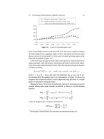
Figure 7.3. Lysine transaction prices in the U.S. and EU markets 1991–95.
Source: Connor (2008).
so could be followed by tacit arrangements or, perhaps more innocently, competitive
costs went up considerably during those years for other reasons. One thing is clear,
depending on the court’s view of the end date for collusive prices, the damages
calculation clearly looks materially different. (For a detailed description of the case,
see Taylor and Yokell (1979).)
Some price series will be even less obvious to interpret.
5
Figure 7.3, for example,
shows the transaction prices of lysine, a farm feed additive, in the United States
and European Union markets between 1991 and 1996. The figure shows successive
periods of sharp price drops followed by sharp price increases. In itself the time
series of prices does not present an obvious picture of what the “but for” prices

should be or even of the exact period of the cartel. One must know some of the facts
of the case to start making sense of the picture.
In 1991, ADM entered the lysine market by building a very large new plant for
lysine production that doubled the world’s production capacity.
6
After starting sales
at very low prices, ADM started communicating that it was willing to coordinate
its entry to the market with competitors. ADM used the threat of its large capacity
to convince competitors that they would be better off in a coordinated agreement
than in a world of competition. ADM even offered its competitors tours of their
large new plant to emphasize the point. The cartel worked quite well but eventually
attracted the attention of authorities. The spectacular investigation in the United
States, which involved the FBI’s undercover agents, moles, and secret recordings,
was made public in 1995.
5
This discussion draws on Connor (2008).
6
European Commission Decision 2001/418/EC, 7/6/2000, L 152/24.
356 7. Damage Estimation
Knowingthese factsperhaps makesfigure 7.3 more understandable. There is a first
attempt at raising prices in 1992 followed by a temporary collapse of the conspiracy
and resumption in mid 1993. The cartel happily goes on until early 1995 when the
investigation ismadepublic.Ofcourse,evenifwecanestablisha clear understanding
of the patterns in the price data shown in figure 7.3, it does not immediately provide
a clear answer to the question of what the “but for” price should be. For example,
before the first known attempt at coordination by ADM, there is a sharp fall in prices,
which was caused by ADM’s entry. However, was ADM entering at artificially low
prices or was the massive but perhaps ultimately temporary excess capacity keeping
prices artificially low post entry? In the other direction, one might wonder whether
the 1991 prices before entry were competitive or whether price fixing activities

were already taking place. In fact, there is allegedly some evidence to suggest that
the main suppliers of lysine were already coordinating and had orchestrated the
sharp increase in prices in 1991. It is not clear that there is a particular moment
when the market would have been clearly in competitive equilibrium in these data
and, as a result, the before-and-after method should probably only be used after an
appropriately careful and rigorous analysis. At trial, the plaintiffs used the periods
May–June 1992 and April–July 1993 as the “but for” price, claiming that there has
been a reversion to competition during these periods. The defendants, on the other
hand, claimed that aggressive competition was not the most likely equilibrium “but
for” scenario in this concentrated oligopolistic industry.
7
There is relatively little economic theory in the “before-and-after” methodology
although in some special cases the results are very intuitive and may even be fairly
accurate. In other contexts, there are cases where a purely statistical approach to
forecasting can sometimes perform better than building an economic model and
basing the forecast on that. Either approach requires assumptions. For example,
the raw form of the before-and-after methodology implicitly assumes that mar-
ket conditions are unchanged since if demand and supply conditions vary during
the cartel period or between the competition and cartel periods, the methodol-
ogy is bound to be incorrect to at least some extent. Naturally, if the cartel has
a long duration, then it is more likely that conditions in the market changed mate-
rially during the period. If a cartel has been around for a long time, the level of
prices outside of the period of the illegal conduct will be probably less indica-
tive of what would have happened during the cartel period if competition had
prevailed.
7.1.2.3 Multivariate Approach
One can attempt to overcome the criticisms of the simplest version of the “before-
and-after” method by taking into account changes in demand and supply conditions.
By running a reduced-form regression of the price level on demand and cost factors
7

For a good discussion of the overcharge estimation in lysine cartel case, see Connor (2004).
7.1. Quantifying Damages of a Cartel 357
that affect the price but are not controlled by the cartel and then also including a
dummy variable for the time of the cartel. The dummy variable will, we hope, then
capture the magnitude the unexplained increase in prices that occurs during the
cartel. The regression run is as follows:
p
t
D ˛ CD
t
C x
t
ˇ C"
t
;
where D
t
is a dummy variable taking on the value 1 if the cartel is active in period
t and 0 otherwise and x
t
is a vector of demand and cost factors that affect the price
but are not controlled by the cartel. The coefficient  will give the amount of the
overcharge per period.
Economic experts working for the defendant will typically want to include a lot
of variables in x in an attempt to reduce the size and significance of the coefficient
 and thereby show no or few damages are due. It is important that no irrelevant
variables are included in the regression, particularly those which might be spuriously
correlated with the cartel dummy D
t
. Also results from a reduced-form regression

should be robust to small changes in the specification of the regression. We discussed
regression analysis in more detail in chapter 2.
Such an approach, of course, raises the question of whether the impact of the cartel
can be well captured by a discrete upward shift of the price during the cartel. The
coefficient  on the dummy variable will measure the average price increase during
the entire selected duration of the cartel, independently of movements in market
conditions that may have occurred during that time. But it is likely that changes
in demand and supply will affect the impact of the cartel on the prices and that a
richer specification would capture a more complex effect. Also, cartels may unwind
slowly so that in the last months or even years of a cartel the overcharge is gradually
decreasing. A dummy specification assigns the same magnitude of the cartel effect
to all years and will return only an average for the entire period. Although it is still
relatively uncommon to perform more elaborate regressions, it is important that the
results of the reduced form be at least compared with alternative specifications to
check for robustness.
A second multivariate approach is to forecast the “but for” price that would have
prevailed during the cartel period absent the conspiracy. Using pre-cartel and post-
cartel data the effect of the determinants of demand and cost shifters on price can
be estimated. Those values of the parameters can be used to predict the “but for”
price during the cartel. The difference between the actual price and the predicted
price provides a prediction of the overcharge. As opposed to the simple before-and-
after method, forecasting the price by running multivariate regression can allow for
changes in the demand and supply conditions. However, it assumes that the structural
relation between the variables remains unchanged. In particular, it supposes that the
conduct of the firms and that the way demand and costs affect prices would each
have remained stable. Such an assumption would clearly be violated if there was a
big technological change or a substantial shift in the tastes of consumers.
358 7. Damage Estimation
Weighted average unit price ($/kg)
1981

1980
1983
1982
1985
1984
1987
1986
1989
1988
1991
1990
1993
1992
1995
1994
1997
1996
1999
1998
2001
2000
Plea-era period
0
10
20
5
15
40
25
30

35
Actual price
Model ‘‘but for’’ price
Straight-line ‘‘but for’’ price
Conspiracy period
Plea-era period
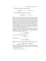
Figure 7.4. Vitamin E acetate oil USP price and “but for” price.
Source: Figure 14.2 of Bernheim (2002), also cited in Connor (2008).
A “but for” estimation was performed in the context of the vitamin cartel in the
1990s. In his expert report for the Vitamin Antitrust Litigation, Professor Bernheim
(2002) estimated the prices that would have prevailed absent the conspiracy using
reduced-form regressions. The price regression was specified as follows:
P
t
D ˛P
t1
C ˇx
t1
C "
t
;
where P
t
is the price of the vitamin product in month t and x
t
are exogenous supply
and demand variables. Exogenous determinants of supply are the price of traded raw
materials needed to manufacture the vitamins, the wage index for the industry, the
interest rate, and exchange rates with currencies where manufacturers are located.
Many potential determinants of demand are also considered: population size, income

per capita, pounds of different slaughtered animals that feed on those vitamins,
quantity produced of pharmaceuticals, and quantity produced of products that use
vitamins as an input such as toiletries, cheese, and milk. The price of substitute
products are also included such as wheat, corn, soybean, a series of vegetables and
fruit, as well as other food products.
A new element of this specification compared with our earlier specifications is the
lagged price variable. Introducing a lagged endogenous variable introduces some
dynamics into the model and means, for example, that shocks to prices will persist.
In fact, the lagged price term not only included the lagged price of the product in
question but also the lagged prices of all the vitamin products within the same family
of vitamins. To estimate the model Bernheim used the data from before the cartel and
also the data available twelve months after the end of the cartel for those products
where there are more than two manufacturers and post-cartel tacit coordination is
assumed to have been ineffective. The predicted prices for a type of vitamin E during
the cartel period using the Bernheim model are shown in figure 7.4.
7.1. Quantifying Damages of a Cartel 359
0
10
20
30
50
Weighted average unit price ($/kg)
1981
40
60
1980
1983
1982
1985
1984

1987
1986
1989
1988
1991
1990
1993
1992
1995
1994
1997
1996
1999
1998
2001
2000
Actual price
Model ‘‘but for’’ price
Straight-line ‘‘but for’’ price
Plea-era sales value:
$43,308,358
Manufacturers
Cartel
(product level)
Roche
BASF
Noncartel
(vitamin level)
China (after 88)
Russia (after 90)

India (after 95)
Glaxo
Others
Conspiracy period
Plea-era period
Plea-era period
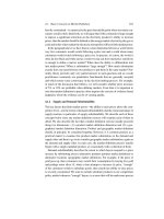
Figure 7.5. Vitamin A acetate 500 USP price and “but for” price.
Source: Figure 14.6 of Bernheim (2002), also cited in Connor (2008).
The specification in the Bernheim report includes quite a number of explanatory
variables, although the actual results of the regression are not reported in the pub-
licly available testimony. The sharp upward shift of the “but for” price before the
actual price is actually raised, for example, must be due to one or more variables
in the model. In any exercise like this, it would be very interesting to see how well
the model can predict actual prices in the period prior to the cartel. The method-
ology appears on the face of it to produce reasonable results, though as observers
not steeped in the detail we probably conclude the results are reasonable at least
partly because the resulting “but for” world is in fact not so different from the one
estimated through a simple “before-and-after” analysis using a straight-line “but
for” price.
The same cannot be said immediately of the “but for” prices predicted for the
vitamin A acetate 500 USP, which is presented in figure 7.5. The predicted prices
appear to extrapolate the trend in pre-cartel prices throughout the period of the cartel.
In this case, post-cartel prices were not used to estimate the model since only two
manufacturers produced it and therefore there was no presumption of reversion to
a competitive scenario at the end of the cartel. Of course, in order to believe the
results emerging from this model we really need to believe that whichever variable
is driving the predicted “but for” prices to trend down captures a real driving force
for competitive prices.
These examples help illustrate that the estimation of a “but for” price using mul-
tivariate regression leaves plenty of room for reasonable people to hold a debate

about the right measure of damage. That said, it can be a very effective tool when
applied correctly. As with any powerful tool, it needs to be used with a great deal of
care and in particular a very good understanding of the data, institutions, and facts
of the case.
360 7. Damage Estimation
7.1.2.4 Yardsticks
When the cartel does not appear to have been equally stable during all years or when
the demand and supply conditions have fluctuated in a significant way during the
cartel, extrapolating the “but for” price from prices prevailing before or after the
cartel will not produce the right answer. An alternative method is to choose a price
of a related product, a product that was not included in the cartel, and use it as a
benchmark to construct what would have happened to the price of the cartelized
good in the event of competition. A price will be a good benchmark if the product
is closely related to the product object of the cartel. It must be similar in terms of
demand, costs, and market structure. Generally, it must be in the same region or
country so that main shocks and institutional factors are similar. The market must
be expected to have behaved in a manner similar to the cartelized market had it not
been cartelized.
Let us consider an example based on the steel cartel.
8
There was allegedly a series
of meetings in the steel industry in the 1990s during which sensitive information
was exchanged between competitors. Volume information and price targets of some
steel products in the European Union were discussed. The economic experts ran a
linear regression as follows:
Price
ij k l t
D ˛ Cˇ Costs
ij k l t
C  Demand

ij k l t
C ı Bargaining power
ij k l t
C  Discussions
ij k l t
C Â
k
Trend
t
C 
i
C Á
j
C 
k
C 
t
C "
ij k l t
;
where i indicates the product, j the subsidiary, k the country, l the client, and
t is the time period. The data vary both across time and across products so the
regression can use a combination of the data variation used for both the “before-
and-after” method and also the benchmark approach. In addition, the data vary
across subsidiaries, countries, and clients (customers). The coefficient  captures
the effect of a meeting on the price level of the good. In this specification, the effect
is taken to be contemporaneous so that discussions during time period t are assumed
to affect prices during time period t. The direct effect of the cartel will be given by
the magnitude of the coefficient , which one would hope would be statistically
significant if there are enough data to pick up the effects. Such a specification is

certainly open for debate and indeed econometric specification testing. For example,
the analyst may wish to explore whether the effect of the cartel on prices captured
in this specification as an indicator variable which takes the value 1 when cartel
members held discussions or whether the effects of discussions are likely to be
something closer to an investment which accumulates over time, but perhaps also
depreciates at some rate. Such questions regarding the appropriate “modeling” of
the effects of cartel discussions on cartel outcomes is difficult to evaluate in the
abstract but must be considered during a case, upon whose facts the correct answer
8
This example is based on LECG’s presentation by David Sevy at the Association of Competition
Economists Conference in Copenhagen in 2005.
7.1. Quantifying Damages of a Cartel 361
will depend. We put “modeling” deliberately in quotes because we always have to
bear in mind that this is a reduced-form regression equation, not a structural price
equation. In principle a structural model of prices could also be builtandthatprovides
another route to damage calculation which we study below (see section 7.1.2.6).
Note that the regression has separate fixed effects for products, subsidiaries,
clients, and country as opposed to fixed effects for a given product in a given sub-
sidiary delivered for a given customer, which would involve an awful lot more fixed
effects. This specification puts more structure on the nature of data variation and
allows different sources of data variation to identify the coefficient . It would prob-
ably be helpful to try specifications with various types of fixed effects in order to
isolate the source of the data variation that is helping to identify . Doing so helps
us, for example, understand whether we are using primarily time-series variation
as in the “before-and-after” method or else cross-sectional variation, which is more
akin to the yardstick approach. A good way to understand what drives the results we
find is to run the regression without any dummies and add the dummies sequentially
taking the data variation one dimension at a time. First, we can control for products,
then for countries, then for subsidiary, and finally for customer. Naturally, the less
sensitive the estimate of  is to changes in the specifications, the more the data vari-

ation in all directions agrees and hence we can be confident that we have identified
the correct effect. However, if the estimate of  does change according to the types
of fixed effects included, as it will on many occasions, it helps us understand where
the data variation suggesting “bad” effects of the cartel is coming from and this may
in turn help us evaluate whether we believe the results are truly capturing the effect
of the cartelists’ discussions on the price.
To calculate damages, we need to estimate the price for each product, subsidiary,
country, and customer using the estimated coefficients but setting the coefficient 
to 0. In this example, the predicted “but for” price was calculated using the formula:
Price
Comp
ij k l t
DO˛ C
O
ˇ Costs
ij k l t
CO Demand
ij k l t
C
O
ı Bargaining power
ij k l t
C 0 Discussions
ij k l t
C
O
Â
k
Trend
t

CO
i
COÁ
j
CO
k
CO
t
:
And so the damages for each particular product and customer at a specific time will
be calculated as
Damages
ij k l t
D .Price
Cartel
ij k l t
 Price
Comp
ij k l t
/Q
Cartel
ij k l t
:
Equivalently, of course, since with our definitions,  D .Price
Cartel
ij k l t
Price
Comp
ij k l t
/, one

can just multiply  by the quantity sold during the cartel period to get an aggregate
damage figure for the cartel.
7.1.2.5 Cost Plus Method
Another method for constructing a “but for” price adds an estimated margin to the
costs of the firm. This method presupposes that the expert can (1) estimate costs of
362 7. Damage Estimation
the firm and (2) estimate the profitability of the firm absent the conspiracy since the
method usually involves using cost data and then adding to it a “reasonable” rate of
return. In general, neither costs nor an appropriate margin are by any means easy to
measure.
Margins are not only dependent on the market structure but given a particular form
of oligopolistic competition they also vary with supply and demand conditions. Peri-
ods of high demand may tend to increase margins.
9
Fixed costs arising from lumpy
investments will typically also be relevant and difficult to take into account because
they transcend a nice clean time period for analysis. For example, the economics
are pretty clear in ensuring that industries such as pharmaceuticals will tend to have
high margins but also incur a great deal of expenditure undertaking often highly
speculative research and development for which a “reasonable” rate of return will
need to be allowed (see, for example, Ashurst 2004). Of course, a cartel in one
submarket might argue that the returns are needed to finance research across their
product line. Portfolio effects of this form and lumpy investment expenditure make
damage estimation in such contexts extremely difficult, although some companies’
internal systems may help address these kinds of issues. For example, some com-
panies use activity-based costing (ABC) methods in accounting to systematically
allocate costs, including fixed costs, to each of their activities. Other contexts may
introduce other difficulties. For example, the rate of return that companies would
obtain in a world without a cartel will depend on the type of competition the firms
would face. If the alternative to cartel is perfect competition, “reasonable” returns

should be lower than if the firms had found themselves playing a Cournot game
or some other form of oligopolistic competition. The economic expert will need to
clearly justify any choice of “reasonable rate of return” but such judgments may be
difficult even if the aim is realistically to determine an order of magnitude.
While “reasonable” rates of return may be difficult in practice, even conceptually
the right choice of the cost measure may be difficult. One could, on the basis of
economic theory, argue that the right costs for damage calculations are marginal
costs or perhaps long-run incremental costs. Alternatively, one might reasonably
decide that the average cost is the best measure since firms that will survive in
the market cannot make losses for a long time.
10
As a general rule, one should
not include costs that are irrecoverable given movements in, say, technology, i.e.,
those costs which are sunk and would not be recovered under competition should
be excluded from the cost calculation since well-functioning markets are forward
9
In fact, the observation that margins tend to vary with the business cycle has also motivated some of
the literature on collusion (see, for example, Rotemberg and Saloner 1986).
10
The usual prediction that competitive firms price at marginal cost ignores the requirement that profits
be positive. For example, if marginal costs are constant and a firm sets prices by maximizing profit subject
to profits being at least zero, then with fixed costs the familiar prediction that p D c will never cover fixed
costs and so will not be optimal. Deciding when to take into account the “profits must be nonnegative”
constraint is important since it fundamentally changes the theory’s prediction for pricing whenever there
are fixed costs of production.