Micowave and Millimeter Wave Technologies Modern UWB antennas and equipment Part 10 potx

MicrowaveandMillimeterWaveTechnologies:ModernUWBantennasandequipment262

Because the modulation scheme discussed in section 3.2 is adopted, pure 40-GHz reference
can be yielded together with the 37.5-GHz modulated signal in BS. Unlike the BS design in
section 3.1, both 40-GHz carrier and 37.5-GHz modulated signals are transmitted from BS to
MT in this system. Therefore, the 40-GHz carrier can be used as mm-wave reference for both
BS and MT. In the uplink, each BS transmits the down-converted 2.5-GHz signal back to CS
with a different wavelength.

4. Millimeter-wave fading induced by fiber chromatic dispersion in RoF
system

The fiber chromatic dispersion is always one of critical problems in optical communications.
Optical components at different frequencies travel through the fiber at different velocities. A
pulse of light broadens and becomes distorted after passing through a single-mode fiber
(Meslener, 1984). To mm-wave RoF system, the fiber chromatic dispersion causes the
remarkable mm-wave fading (Schmuck, 1995).

4.1 Analysis of chromatic dispersion in intensity modulated RoF system
The intersity modulation schemes of yielding mm-wave signal have been introduced in
Section 2.1. Those schemes may be sensitive to fiber chromatic dispersion. For example, an
external optical modulator (MZM) is used to modulate CW optical signal with a RF signal.
The electric field at the output of optical modulator is express as (Schmuck, 1995)

( ) cos[ cos ] cos
2 2
c m c
E
t E d m t t





    
(16)

where
c
E
is the amplitude of electric field;
c

is the central angular frequency of optical
source;
s

is the angular frequency of RF signal;
/
m
m V V


is normalized amplitude of the
driving RF signal;
/
b
d V V


is the normalized bias voltage of the modulator;

V

is the

shift voltage of the modulator.
The electric field for
/ 2
b
V V


, after the transmission over a fiber link can be expressed by
Bessel functions

0 0 1 1 2
( ) ( )cos( ) ( ){cos[( ) ] cos[( ) ]}
2 2
c c
c c m c m
E E
E t J t J t t
         
       
(17)

where / 2m


 ;
0


,
1

and
2

represent the different phase delays of the optical
components due to the fiber chromatic dispersion.
After photo-detection at the PD, the power of wished mm-wave signal can be approximately
expressed as
2 2
2 2 2
cos [ ( ) ] cos [ ]
m c m
c
f
D f z
p cD z
f c
 

 
(18)

where D represents the fiber group velocity dispersion parameter; c is the velocity of light in
vacuum;
c

is wavelength and z is the fiber length. If parameters are chosen as: c=3x10

8
-m/s,
D=17-ps/(km
× nm),
c


1550-nm,
m
f

40-GHz, the relation between the amplitude of mm-
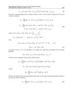
wave and the transmission distance in fiber is shown in Figure 16. It shows that the
amplitude of mm-wave changes with the transmission distance so fast that this mm-wave
generation scheme can not be used in practice.


Fig. 16. The relative amplitude of 40-GHz mm-wave varies with the fiber length

Many methods have been proposed to overcome the mm-wave signal fading induced by
fiber chromatic dispersion. Smith et al. (1997) proposed a method to generate an optical
carrier with single sideband (SSB) modulation by using a DD-MZM, biased at quadrature
point, and applied with RF signals,
/ 2

out of phase to its two electrodes. The RF power
degradation due to fiber dispersion was observed to be only 15-dB when using the
technique to send 2 to 20-GHz signals over 79.6-km of fiber. By using an optical filter to
depress one sideband. SSB optical modulation is realized and demonstrated by Park et al.
(1997). Moreover, stimulated Brillouin scattering (SBS), a nonlinear phenomenon in optical

fiber was applied to realize SSB modulation by Yonenaga & Takachio (1993).

4.2 Fiber chromatic dispersion in OFM techniques
In this section, the chromatic dispersion in OFM techinques will be discussed. According to
the basic arrangement of optical frequency sweeping technique, shown in Figure 6, the
equation (2) can also be expressed as (Walker et al., 1992)

( ) ( ) exp( ) exp[ ( ) ]
in s c n c s
n
E t f t j t F j n t
   


  

(19)
where the harmonic components
n
F
is given by:
1
( ) exp( )
2
n
F f jn d



 



 

(20)
( ) exp( cos ) exp[ cos( ) ]
c c s c
f E j E j j

       
   
(21)
Millimeter-waveRadiooverFiberSystemforBroadbandWirelessCommunication 263

Because the modulation scheme discussed in section 3.2 is adopted, pure 40-GHz reference
can be yielded together with the 37.5-GHz modulated signal in BS. Unlike the BS design in
section 3.1, both 40-GHz carrier and 37.5-GHz modulated signals are transmitted from BS to
MT in this system. Therefore, the 40-GHz carrier can be used as mm-wave reference for both
BS and MT. In the uplink, each BS transmits the down-converted 2.5-GHz signal back to CS
with a different wavelength.

4. Millimeter-wave fading induced by fiber chromatic dispersion in RoF
system

The fiber chromatic dispersion is always one of critical problems in optical communications.
Optical components at different frequencies travel through the fiber at different velocities. A
pulse of light broadens and becomes distorted after passing through a single-mode fiber
(Meslener, 1984). To mm-wave RoF system, the fiber chromatic dispersion causes the
remarkable mm-wave fading (Schmuck, 1995).

4.1 Analysis of chromatic dispersion in intensity modulated RoF system
The intersity modulation schemes of yielding mm-wave signal have been introduced in
Section 2.1. Those schemes may be sensitive to fiber chromatic dispersion. For example, an
external optical modulator (MZM) is used to modulate CW optical signal with a RF signal.
The electric field at the output of optical modulator is express as (Schmuck, 1995)

( ) cos[ cos ] cos
2 2
c m c
E
t E d m t t




    
(16)

where
c
E
is the amplitude of electric field;
c

is the central angular frequency of optical
source;
s

is the angular frequency of RF signal;
/

m
m V V


is normalized amplitude of the
driving RF signal;
/
b
d V V


is the normalized bias voltage of the modulator;
V

is the

shift voltage of the modulator.
The electric field for
/ 2
b
V V


, after the transmission over a fiber link can be expressed by
Bessel functions

0 0 1 1 2
( ) ( )cos( ) ( ){cos[( ) ] cos[( ) ]}
2 2
c c

c c m c m
E E
E t J t J t t

        
       
(17)

where / 2m


 ;
0

,
1

and
2

represent the different phase delays of the optical
components due to the fiber chromatic dispersion.
After photo-detection at the PD, the power of wished mm-wave signal can be approximately
expressed as
2 2
2 2 2
cos [ ( ) ] cos [ ]
m c m
c
f

D f z
p cD z
f c
 

 
(18)

where D represents the fiber group velocity dispersion parameter; c is the velocity of light in
vacuum;
c

is wavelength and z is the fiber length. If parameters are chosen as: c=3x10
8
-m/s,
D=17-ps/(km
× nm),
c


1550-nm,
m
f

40-GHz, the relation between the amplitude of mm-
wave and the transmission distance in fiber is shown in Figure 16. It shows that the
amplitude of mm-wave changes with the transmission distance so fast that this mm-wave
generation scheme can not be used in practice.

Fig. 16. The relative amplitude of 40-GHz mm-wave varies with the fiber length

Many methods have been proposed to overcome the mm-wave signal fading induced by
fiber chromatic dispersion. Smith et al. (1997) proposed a method to generate an optical
carrier with single sideband (SSB) modulation by using a DD-MZM, biased at quadrature
point, and applied with RF signals,
/ 2

out of phase to its two electrodes. The RF power
degradation due to fiber dispersion was observed to be only 15-dB when using the
technique to send 2 to 20-GHz signals over 79.6-km of fiber. By using an optical filter to
depress one sideband. SSB optical modulation is realized and demonstrated by Park et al.
(1997). Moreover, stimulated Brillouin scattering (SBS), a nonlinear phenomenon in optical
fiber was applied to realize SSB modulation by Yonenaga & Takachio (1993).

4.2 Fiber chromatic dispersion in OFM techniques
In this section, the chromatic dispersion in OFM techinques will be discussed. According to
the basic arrangement of optical frequency sweeping technique, shown in Figure 6, the
equation (2) can also be expressed as (Walker et al., 1992)

( ) ( ) exp( ) exp[ ( ) ]
in s c n c s
n
E t f t j t F j n t
   


  

(19)

where the harmonic components
n
F
is given by:
1
( ) exp( )
2
n
F f jn d



 


 

(20)
( ) exp( cos ) exp[ cos( ) ]
c c s c
f E j E j j

       
   
(21)
MicrowaveandMillimeterWaveTechnologies:ModernUWBantennasandequipment264

The fiber transfer characteristic can be written in the form

2

2
0 1
( ) exp[ ( ( ) ( ) ) ]
2
c c
k
H
j k k z
    
      
(22)

where the first term is a constant phase shift, the second term is constant propagation delay
and the third term is the first order dispersion of optical fiber. At the angular frequencies of
side modes in the light-wave, ( )H

has the values:
2 2 2
2
0 1 0 1
( ) exp[ ( ) ] exp[ ( ]
2
n c s s s s
k
H H n j k k n n z j k z k n z n

    
         
(23)
where

2
2
/ 2
s
k z
 

represents the fiber dispersion at the angular frequency of the first side-
mode.
The first order dispersion constant D of fiber is related to
2
k by the
expression
2
2
2 /
c
D ck


 
, therefore

is related to D by

2 2
4
s c
D
z

c
 


  (24)

where c is the light velocity in vacuum, z is the transmission distance in fiber and
c

is the
working wavelength.
The electric field of light-wave at output of the fiber is
( ) exp[ ( ) ]
out n n c s
n
E t F H j n t
 


 

(25)

The photo-current produced in PD is
* * *
( ) ( ) ( ) exp[ ( ) ]
d out out
n m
n m n m s
i t E t E t F F H H j n m t


 
 
  
 
(26)
Setting
p n m  and substituting (20) and (23) for
n
F
and
n
H
in (26) gives

*
1
1
1
( ) ( ) exp( ) exp( ( ))
2
exp( ( ))
( )
s
p
p s
p
d
f
p f p jp d jp t k z

I jp t k z
i t



     







   
 




(27)
Hence the amplitude of p-th harmonic in photo-current after transmission over the fiber
becomes
*
1
( ) ( ) exp( )
2
p
I
f p f p jp d




    


   

(28)
Substituting (21) for
( )f

in (28) and performing the integration give


2
{ (2 sin ) exp( ) (2 sin )
exp( ) (2 sin( ))
2 2
exp( ) (2 sin( ))}
2 2
p c p s p
s s
c p
s s
c p
I
E J p jp J p
j jp J p
j jp J p


    
   
   
   
   
  
  
   
(29)

So the pth harmonic can be approximately expressed by


exp( ) exp( )
p p s p s
F I jp t I jp t



  
(30)

Applying the parity of Bessel function to equation (38),
n
F
can be written as


2
2 { (2 sin )[cos cos( )]

(2 sin( )) cos( )
2 2
(2 sin( )) cos( )}
2 2
p c p s s s
s s
p s c
s s
p s c
F E J p p t p t p
J p p t p
J p p t p

    
   

   
   

   
  
   
   
(31)

The intensity modulation depth
p
M
is defined as
0

| / |
p p
M
F F

. In the condition that the
optimized condition (
,
c s
k

    


) for optical frequency sweeping technique is
satisfied, the intensity


(a) (b)
Fig. 17. The intensity modulation depth of 12th harmonic in the (a) satisfied condition, (b)
unsatisfied condition.

modulation depth of 12th harmonic with transmission distance is shown in Figure 17 (a).
Figure (b) shows the intensity modulation depth in the unsatisfied condition and the odd
harmonics appear.
Lin et al. (2008) analyzed the mm-wave fading caused by fiber chromatic dispersion in the
OFM scheme using nonlinear modulation of DD-MZM. The result is drawn in Figure 18,
Millimeter-waveRadiooverFiberSystemforBroadbandWirelessCommunication 265

The fiber transfer characteristic can be written in the form

2
2
0 1
( ) exp[ ( ( ) ( ) ) ]
2
c c
k
H
j k k z
    
      
(22)

where the first term is a constant phase shift, the second term is constant propagation delay
and the third term is the first order dispersion of optical fiber. At the angular frequencies of
side modes in the light-wave, ( )H

has the values:
2 2 2
2
0 1 0 1
( ) exp[ ( ) ] exp[ ( ]
2
n c s s s s
k
H H n j k k n n z j k z k n z n

    
         

(23)
where
2
2
/ 2
s
k z
 

represents the fiber dispersion at the angular frequency of the first side-
mode.
The first order dispersion constant D of fiber is related to
2
k by the
expression
2
2
2 /
c
D ck


 
, therefore

is related to D by

2 2
4
s c

D
z
c
 


  (24)

where c is the light velocity in vacuum, z is the transmission distance in fiber and
c

is the
working wavelength.
The electric field of light-wave at output of the fiber is
( ) exp[ ( ) ]
out n n c s
n
E t F H j n t
 


 

(25)

The photo-current produced in PD is
* * *
( ) ( ) ( ) exp[ ( ) ]
d out out
n m

n m n m s
i t E t E t F F H H j n m t

 
 
  
 
(26)
Setting
p n m  and substituting (20) and (23) for
n
F
and
n
H
in (26) gives

*
1
1
1
( ) ( ) exp( ) exp( ( ))
2
exp( ( ))
( )
s
p
p s
p
d

f
p f p jp d jp t k z
I jp t k z
i t



     







   
 




(27)
Hence the amplitude of p-th harmonic in photo-current after transmission over the fiber
becomes
*
1
( ) ( ) exp( )
2
p
I

f p f p jp d



    


   

(28)
Substituting (21) for
( )f

in (28) and performing the integration give


2
{ (2 sin ) exp( ) (2 sin )
exp( ) (2 sin( ))
2 2
exp( ) (2 sin( ))}
2 2
p c p s p
s s
c p
s s
c p
I
E J p jp J p
j jp J p

j jp J p

    
   
   
   
   
  
  
   
(29)

So the pth harmonic can be approximately expressed by


exp( ) exp( )
p p s p s
F I jp t I jp t
 

  
(30)

Applying the parity of Bessel function to equation (38),
n
F
can be written as


2

2 { (2 sin )[cos cos( )]
(2 sin( )) cos( )
2 2
(2 sin( )) cos( )}
2 2
p c p s s s
s s
p s c
s s
p s c
F E J p p t p t p
J p p t p
J p p t p

    
   
    
   
    
  
   
   
(31)

The intensity modulation depth
p
M
is defined as
0
| / |

p p
M
F F
. In the condition that the
optimized condition (
,
c s
k

    
 
) for optical frequency sweeping technique is
satisfied, the intensity


(a) (b)
Fig. 17. The intensity modulation depth of 12th harmonic in the (a) satisfied condition, (b)
unsatisfied condition.

modulation depth of 12th harmonic with transmission distance is shown in Figure 17 (a).
Figure (b) shows the intensity modulation depth in the unsatisfied condition and the odd
harmonics appear.
Lin et al. (2008) analyzed the mm-wave fading caused by fiber chromatic dispersion in the
OFM scheme using nonlinear modulation of DD-MZM. The result is drawn in Figure 18,
MicrowaveandMillimeterWaveTechnologies:ModernUWBantennasandequipment266

together with the result of double side-modes IM (without carrier depression) for
comparison. It can be seen in Figure 18 that in the double side-modes IM scheme the
amplitude of generated 40-GHz mm-wave behaves 100% fading with periodic zeros at
different fiber lengths. In contrast, in OFM scheme using DD-MZM, the amplitude fading of

generated 40-GHz mm-wave is much weaker, only 30% and without zeros. Furthermore, the
minimum amplitude happens in much longer period. This means that OFM by using DD-
MZM is a good mm-wave generation method with tolerability to fiber chromatic dispersion.
Conceptually, OFM by using DD-MZM is such a system that generation of mm-wave is the
superposition of several mm-waves generated by self-heterodyne of several pairs of optical
side-modes. So the interference of several mm-waves at the same frequency results in only a
little amplitude fading.


Fig. 18. Amplitude of 40GHz mm-wave varies with fiber length in double side-modes IM
scheme and DD-MZM OFM scheme.

5. Fast handover in mm-wave RoF system

There is much more free space loss at mm-wave band than that at 2.4-GHz or 5-GHz, since
free space loss increases drastically with frequency. In principle this higher free space loss
can be compensated for by the use of antennas with stronger pattern directivity while
maintaining small antenna dimensions. When such antennas are used, however, antenna
obstruction (e.g., by a human body) and mispointing may easily cause a substantial drop of
received power, which may nullify the gain provided by the antennas. This effect is typical
for mm-wave signals because the diffraction of mm-wave signals (i.e., the ability to bend
around edges of obstacles) is weak (Smulders, 2002), so a mm-wave communication
network has many characteristics quite different from conventional wireless LANs (WLANs)
operating in 2.4 or 5-GHz bands.
Due to the free space loss of mm-wave signal, the coverage of BS, as pico-cell has been
smaller than that of Access Point (AP) in current WLAN. The small size of pico-cell induces
the large number of BSs and frequent handovers of MT from one pico-cell to another. As a
result, the key point in designing the Medium Access Control (MAC) protocol for mm-wave
RoF system is to provide efficient and fast handover support. A MAC protocol based on
Frequency Switching (FS) codes can realize fast handover and adjacent pico-cells employ

orthogonal FS codes to avoid possible co-channel interference (Kim & Wolisz, 2003). A
moveable cells scheme based on optical switching architecture can realize the handover in
the order of ns or
μs
(Lannoo et al., 2004), which is suitable to all MTs moving at the same
speed, for example in a train scenario. In this way, MT can operate on the same frequency
during the whole connection and avoid the fast handovers. Based on moveable cells scheme,
Yang & Liu (2008) proposed a further scheme, in which the adjacent pico-cells are grouped
as a larger cell, and along the railway all the BS in this larger cell use the same frequency
channel. When n adjacent pico-cells are grouped, times of handover can be decreased n-fold.

6. Conclusion

In this chapter, many technical issues about the mm-wave RoF systems are presented. Firstly,
three kinds of mm-wave generation techniques are introduced. In those techniques, OFM
techniques realized by optical frequency sweeping and nonlinear modulation of DD-MZM are
mainly discussed and the latter is proved to be a more stable and cost-efficient way to yield
signal at the mm-wave band. Unlike most research works by now only concentrating on the
downlink of RoF system, the design of several bidirectional mm-wave RoF systems is described
which deals with the uplink as optical transport of IF signal, generated by down-conversion of
mm-wave signal. The information-bearing mm-wave for radiation and the reference mm-wave
for down-conversion are all generated in BS by OFM. Then, two multiplexing techniques, WDM
and SCM are introduced to mm-wave RoF systems. Star-tree and ring architectures are adopted
in mm-wave RoF systems to realize the distributed BSs. After showing the large bandwidth
capacity at mm-wave band provided by OFM techniques, incorporating SCM to RoF system is
demonstrated to improve the utilization ratio of large bandwidth. Considering the influence of
chromatic dispersion in fiber on mm-wave fading, a common analysis on the effect of fiber
chromatic dispersion to mm-wave generation techniques (i.e., intensity modulation and OFM)
are given and OFM by using DD-MZM is proved to be tolerable to fiber chromatic dispersion.

Due to the great free space loss of signal at mm-wave band, the coverage of each BS is very small
and the handover of MT becomes a problem. To meet the real-time communication requirements
for mm-wave systems, several MAC protocols suitable either to efficient and fast handover or to
moveable cells schemes, which make the MT avoid the fast handover problem, are introduced.

7. Acknowledgements

This work was surpported by the National Natural Science Foundation of China (60377024
and 60877053), and Shanghai Leading Academic Discipline Project (08DZ1500115).

8. References

Braun, R P.; Grosskopf, G.; Heidrich, H.; von Helmolt, C.; Kaiser, R.; Kruger, K.; Kruger, U.;
Rohde, D.; Schmidt, F.; Stenzel, R. & Trommer, D. (1998). Optical microwave
generation and transmission experiments in the 12- and 60-GHz region for wireless
communications, Microwave Theory and Techniques, IEEE Transactions on, Vol. 46, No.
4, pp. 320-330.
Millimeter-waveRadiooverFiberSystemforBroadbandWirelessCommunication 267

together with the result of double side-modes IM (without carrier depression) for
comparison. It can be seen in Figure 18 that in the double side-modes IM scheme the
amplitude of generated 40-GHz mm-wave behaves 100% fading with periodic zeros at
different fiber lengths. In contrast, in OFM scheme using DD-MZM, the amplitude fading of
generated 40-GHz mm-wave is much weaker, only 30% and without zeros. Furthermore, the
minimum amplitude happens in much longer period. This means that OFM by using DD-
MZM is a good mm-wave generation method with tolerability to fiber chromatic dispersion.
Conceptually, OFM by using DD-MZM is such a system that generation of mm-wave is the
superposition of several mm-waves generated by self-heterodyne of several pairs of optical
side-modes. So the interference of several mm-waves at the same frequency results in only a
little amplitude fading.

Fig. 18. Amplitude of 40GHz mm-wave varies with fiber length in double side-modes IM
scheme and DD-MZM OFM scheme.

5. Fast handover in mm-wave RoF system

There is much more free space loss at mm-wave band than that at 2.4-GHz or 5-GHz, since
free space loss increases drastically with frequency. In principle this higher free space loss
can be compensated for by the use of antennas with stronger pattern directivity while
maintaining small antenna dimensions. When such antennas are used, however, antenna
obstruction (e.g., by a human body) and mispointing may easily cause a substantial drop of
received power, which may nullify the gain provided by the antennas. This effect is typical
for mm-wave signals because the diffraction of mm-wave signals (i.e., the ability to bend
around edges of obstacles) is weak (Smulders, 2002), so a mm-wave communication
network has many characteristics quite different from conventional wireless LANs (WLANs)
operating in 2.4 or 5-GHz bands.
Due to the free space loss of mm-wave signal, the coverage of BS, as pico-cell has been
smaller than that of Access Point (AP) in current WLAN. The small size of pico-cell induces
the large number of BSs and frequent handovers of MT from one pico-cell to another. As a
result, the key point in designing the Medium Access Control (MAC) protocol for mm-wave
RoF system is to provide efficient and fast handover support. A MAC protocol based on
Frequency Switching (FS) codes can realize fast handover and adjacent pico-cells employ

orthogonal FS codes to avoid possible co-channel interference (Kim & Wolisz, 2003). A
moveable cells scheme based on optical switching architecture can realize the handover in
the order of ns or
μs
(Lannoo et al., 2004), which is suitable to all MTs moving at the same
speed, for example in a train scenario. In this way, MT can operate on the same frequency

during the whole connection and avoid the fast handovers. Based on moveable cells scheme,
Yang & Liu (2008) proposed a further scheme, in which the adjacent pico-cells are grouped
as a larger cell, and along the railway all the BS in this larger cell use the same frequency
channel. When n adjacent pico-cells are grouped, times of handover can be decreased n-fold.

6. Conclusion

In this chapter, many technical issues about the mm-wave RoF systems are presented. Firstly,
three kinds of mm-wave generation techniques are introduced. In those techniques, OFM
techniques realized by optical frequency sweeping and nonlinear modulation of DD-MZM are
mainly discussed and the latter is proved to be a more stable and cost-efficient way to yield
signal at the mm-wave band. Unlike most research works by now only concentrating on the
downlink of RoF system, the design of several bidirectional mm-wave RoF systems is described
which deals with the uplink as optical transport of IF signal, generated by down-conversion of
mm-wave signal. The information-bearing mm-wave for radiation and the reference mm-wave
for down-conversion are all generated in BS by OFM. Then, two multiplexing techniques, WDM
and SCM are introduced to mm-wave RoF systems. Star-tree and ring architectures are adopted
in mm-wave RoF systems to realize the distributed BSs. After showing the large bandwidth
capacity at mm-wave band provided by OFM techniques, incorporating SCM to RoF system is
demonstrated to improve the utilization ratio of large bandwidth. Considering the influence of
chromatic dispersion in fiber on mm-wave fading, a common analysis on the effect of fiber
chromatic dispersion to mm-wave generation techniques (i.e., intensity modulation and OFM)
are given and OFM by using DD-MZM is proved to be tolerable to fiber chromatic dispersion.
Due to the great free space loss of signal at mm-wave band, the coverage of each BS is very small
and the handover of MT becomes a problem. To meet the real-time communication requirements
for mm-wave systems, several MAC protocols suitable either to efficient and fast handover or to
moveable cells schemes, which make the MT avoid the fast handover problem, are introduced.

7. Acknowledgements

This work was surpported by the National Natural Science Foundation of China (60377024
and 60877053), and Shanghai Leading Academic Discipline Project (08DZ1500115).

8. References

Braun, R P.; Grosskopf, G.; Heidrich, H.; von Helmolt, C.; Kaiser, R.; Kruger, K.; Kruger, U.;
Rohde, D.; Schmidt, F.; Stenzel, R. & Trommer, D. (1998). Optical microwave
generation and transmission experiments in the 12- and 60-GHz region for wireless
communications, Microwave Theory and Techniques, IEEE Transactions on, Vol. 46, No.
4, pp. 320-330.
MicrowaveandMillimeterWaveTechnologies:ModernUWBantennasandequipment268

Doi, M.; Hashimoto, N. ; Hasegawa, T. ; Tanaka, T. & Tanaka, K (2007). 40 Gb/s low-drive-
voltage LiNbO3 optical modulator for DQPSK modulation format. in Optical Fiber
Communication Conference and Exposition and The National Fiber Optic Engineers
Conference, OSA Technical Digest Series (CD), paper OWH4.
Elrefaie, A.F.; Wagner, R.E.; Atlas, D.A. & Daut, D.G. (1988). Chromatic dispersion
limitations in coherent lightwave transmission systems, Lightwave Technology,
Journal of, Vol. 6, No. 5, pp. 704-709, 1988.
Fuster, J.M.; Marti, J.; Candelas, P.; Martinez, F.J. & Sempere, L. (2001). Optical generation of
electrical modulation formats, 27th European Conference on Optical Communication
(ECOC 2001), pp. 536-537, 2001.
Garcia Larrode, M.; Koonen, A.M.J.; Vegas Olmos, J.J.; Tafur Monroy, I. & Schenk, T.C.W.
(2005). RF bandwidth capacity and SCM in a radio-over-fibre link employing
optical frequency multiplication, Conference on Optical Communication, 2005 (ECOC
2005), Vol. 3, pp. 681-682, Sep. 25-29, 2005.
Gliese, U.; Nielsen, T. N.; Bruun, M.; Lintz Christensen, E.; Stubkjaer, K. E.; Lindgren, S. &
Broberg, B. (1992). A wideband heterodyne optical phase-locked loop for
generation of 3-18 GHz microwave carriers, IEEE Photonics Technology Letters, Vol.
4, No. 8, pp. 936-938.

Gliese, U.; Norskov, S. & Nielsen, T.N. (1996). Chromatic dispersion in fiber-optic
microwave and millimeter-wave links, Microwave Theory and Techniques, IEEE
Transactions on, Vol. 44, No. 10, pp. 1716-1724.
Griffin, R.A.; Lane, P.M. & O’Reilly, J.J. (1999). Radio-over-fiber distribution using an optical
millimeterwave/DWDM overlay, OFC 1999, Paper WD6-1, 1999.
Hartmannor, P. ; Webster, M. ; Wonfor, A. ; Ingham, J.D. ; Penty, R.V. ; White, I.H. ; Wake,
D. & Seeds, A.J. (2003). Low cost multimode fibre based wireless LAN distribution
system using uncooled, directly modulated DFB laser diodes, 2003 European
Conference on Optical Communication (ECOC 2003), Sep. 21-25, 2003.
Juha Rapeli (2001). Future directions for mobile communications business, technology and
research, Wireless Personal Communications, Vol. 17, No. 2-3, pp.155-173.
Kim, H.B. & Wolisz, A., Performance evaluation of a MAC protocol for radio over fiber
wireless LAN operating in the 60-GHz band, Global Telecommunications Conference,
2003 (GLOBECOM '03), Vol. 5, pp. 2659-2663, Dec. 1-5, 2003.
Kitayama, K. (1998). Architectural considerations of radio-on-fiber millimeter-wave wireless
access systems, International Symposium on Signals, Systems, and Electronics, 1998
(ISSSE 98), pp.
Kramer, G. (2006). What is next for Ethernet PON?, The Joint Intenational Conference on Optical
Internet and Next Generation Network, 2006 (COIN-NGNCON 2006), pp. 49-54, Jul. 9-
13, 2006.
Kuri, T.; Kitayama, K.; Stohr, A. & Ogawa, Y. (1999). Fiber-optic millimeter-wave downlink
system using 60 GHz-band external modulation, Lightwave Technology, Journal of,
Vol. 17, No. 5, pp. 799-806.
Lannoo, B.; Colle, D.; Pickavet, M. & Demeester, P. (2004). Optical switching architecture to
realize "moveable cells" in a radio-over-fiber network, 6th International Conference on
Transparent Optical Networks, 2004, Vol. 2, pp. 2-7, Jul. 4-8, 2004.

Larrode, M.G.; Koonen, A.M.J.; Olmos, J.J.V.; Verdurmen, E.J.M. & Turkiewicz, J.P. (2006).
Dispersion tolerant radio-over-fibre transmission of 16 and 64 QAM radio signals at
40 GHz, Electronics Letters, Vol. 42, No. 15, pp. 872-874.

Lin, Ru-jian; Zhu, Mei-wei; Zhou, Zhe-yun & Ye, Jia-jun (2008). Theoretic and experimental
study on mm-wave radio over fiber system based on OFM, Proc. SPIE, Vol. 7137,
71371M (2008), DOI:10.1117/12.807835.
Meslener, G. (1984). Chromatic dispersion induced distortion of modulated monochromatic
light employing direct detection, Quantum Electronics, Journal of, Vol. 20, No. 10, pp.
1208-1216, 1984.
Nirmalathas, A.; Lim, C.; Novak, D.; Castleford, D.; Waterhouse, R. & Smith, G. (2000).
Millimeter-wave fiber-wireless access systems incorporating wavelength division
multiplexing, Microwave Conference, 2000 Asia-Pacific, pp. 625-629, 2000.
Ogusu, M.; Inagaki, K.; Mizuguchi, Y. & Ohira, T. (2003). Carrier generation and data
transmission on millimeter-wave bands using two-mode locked Fabry-Perot slave
lasers, IEEE transactions on microwave theory and techniques, Vol. 51 (1), No. 2, pp.
382-391.
Olshansky, R.; Lanzisera, V.A. & Hill, P.M. (1989). Subcarrier multiplexed lightwave
systems for broad-band distribution, Lightwave Technology, Journal of , Vol. 7, No. 9,
pp. 1329-1342, 1989.
O'Rcilly, J.J.; Lane, P.M.; Heidemann, R. & Hofstetter, R. (1992). Optical generation of very
narrow linewidth millimetre wave signals, Electronics Letters, Vol. 28, No. 25, pp.
2309-2311.
Park, J.; Sorin, W.V. & Lau, K.Y. (1997). Ellimination of the fiber chromatic dispersion
penalty on 1550nm millimeter-wave optical transmission, Electronics Letters, Vol. 33,
No. 6, pp. 512-513, 1997.
Schmuck, H. (1995). Comparison of optical millimeter-wave system concepts with regard to
chromatic dispersion, Eletronics Letters, Vol. 31, No. 21, pp.1848-1849, 1995.
Smith, G.H.; Novak, D. & Ahmed, Z. (1997). Techniques for optical SSB generation to
overcome dispersion penalties in fibre-radio systems, Electronics Letters, Vol. 33, No.
1, pp. 74-75, 1997.
Smith, G.H.; Novak, D. & Lim, C., A (1998). Millimeter-wave full-duplex fiber-radio star-tree
architecture incorporating WDM and SCM, Photonics Technology Letters, IEEE, Vol.
10, No. 11, pp. 1650-1652, 1998.

Smulders, P. (2002). Exploiting the 60 GHz band for local wireless multimedia access:
prospects and future directions, Communications Magazine, IEEE, Vol. 40, No. 1,
pp.140-147.
Sun, C.K.; Orazi, R.J. & Pappert, S.A. (1996). Efficient microwave frequency conversion
using photonic link signal mixing, IEEE Photonics Technology Letters, Vol. 8, No. 1,
pp. 154-156.
Stöhr, A.; Kitayama, K. & Jäger, D. (1998). Error-free full-duplex optical WDM-FDM
transmission using an EA-transceiver, International Topical Meeting on Microwave
Photonics, 1998 (MWP 98), pp. 37-40, Oct. 12-14, 1998.
Ton Koonen; Anthony Ng''oma; Peter Smulders; Henrie van den Boom;
Idelfonso Tafur Monroy & Giok-Djan Khoe (2003). In-house networks using
multimode Polymer Optical Fibre for broadband wireless services, Photonic Network
Communications, Vol. 5, No. 2, pp. 177-187.
Millimeter-waveRadiooverFiberSystemforBroadbandWirelessCommunication 269

Doi, M.; Hashimoto, N. ; Hasegawa, T. ; Tanaka, T. & Tanaka, K (2007). 40 Gb/s low-drive-
voltage LiNbO3 optical modulator for DQPSK modulation format. in Optical Fiber
Communication Conference and Exposition and The National Fiber Optic Engineers
Conference, OSA Technical Digest Series (CD), paper OWH4.
Elrefaie, A.F.; Wagner, R.E.; Atlas, D.A. & Daut, D.G. (1988). Chromatic dispersion
limitations in coherent lightwave transmission systems, Lightwave Technology,
Journal of, Vol. 6, No. 5, pp. 704-709, 1988.
Fuster, J.M.; Marti, J.; Candelas, P.; Martinez, F.J. & Sempere, L. (2001). Optical generation of
electrical modulation formats, 27th European Conference on Optical Communication
(ECOC 2001), pp. 536-537, 2001.
Garcia Larrode, M.; Koonen, A.M.J.; Vegas Olmos, J.J.; Tafur Monroy, I. & Schenk, T.C.W.
(2005). RF bandwidth capacity and SCM in a radio-over-fibre link employing
optical frequency multiplication, Conference on Optical Communication, 2005 (ECOC
2005), Vol. 3, pp. 681-682, Sep. 25-29, 2005.
Gliese, U.; Nielsen, T. N.; Bruun, M.; Lintz Christensen, E.; Stubkjaer, K. E.; Lindgren, S. &

Broberg, B. (1992). A wideband heterodyne optical phase-locked loop for
generation of 3-18 GHz microwave carriers, IEEE Photonics Technology Letters, Vol.
4, No. 8, pp. 936-938.
Gliese, U.; Norskov, S. & Nielsen, T.N. (1996). Chromatic dispersion in fiber-optic
microwave and millimeter-wave links, Microwave Theory and Techniques, IEEE
Transactions on, Vol. 44, No. 10, pp. 1716-1724.
Griffin, R.A.; Lane, P.M. & O’Reilly, J.J. (1999). Radio-over-fiber distribution using an optical
millimeterwave/DWDM overlay, OFC 1999, Paper WD6-1, 1999.
Hartmannor, P. ; Webster, M. ; Wonfor, A. ; Ingham, J.D. ; Penty, R.V. ; White, I.H. ; Wake,
D. & Seeds, A.J. (2003). Low cost multimode fibre based wireless LAN distribution
system using uncooled, directly modulated DFB laser diodes, 2003 European
Conference on Optical Communication (ECOC 2003), Sep. 21-25, 2003.
Juha Rapeli (2001). Future directions for mobile communications business, technology and
research, Wireless Personal Communications, Vol. 17, No. 2-3, pp.155-173.
Kim, H.B. & Wolisz, A., Performance evaluation of a MAC protocol for radio over fiber
wireless LAN operating in the 60-GHz band, Global Telecommunications Conference,
2003 (GLOBECOM '03), Vol. 5, pp. 2659-2663, Dec. 1-5, 2003.
Kitayama, K. (1998). Architectural considerations of radio-on-fiber millimeter-wave wireless
access systems, International Symposium on Signals, Systems, and Electronics, 1998
(ISSSE 98), pp.
Kramer, G. (2006). What is next for Ethernet PON?, The Joint Intenational Conference on Optical
Internet and Next Generation Network, 2006 (COIN-NGNCON 2006), pp. 49-54, Jul. 9-
13, 2006.
Kuri, T.; Kitayama, K.; Stohr, A. & Ogawa, Y. (1999). Fiber-optic millimeter-wave downlink
system using 60 GHz-band external modulation, Lightwave Technology, Journal of,
Vol. 17, No. 5, pp. 799-806.
Lannoo, B.; Colle, D.; Pickavet, M. & Demeester, P. (2004). Optical switching architecture to
realize "moveable cells" in a radio-over-fiber network, 6th International Conference on
Transparent Optical Networks, 2004, Vol. 2, pp. 2-7, Jul. 4-8, 2004.

Larrode, M.G.; Koonen, A.M.J.; Olmos, J.J.V.; Verdurmen, E.J.M. & Turkiewicz, J.P. (2006).
Dispersion tolerant radio-over-fibre transmission of 16 and 64 QAM radio signals at
40 GHz, Electronics Letters, Vol. 42, No. 15, pp. 872-874.
Lin, Ru-jian; Zhu, Mei-wei; Zhou, Zhe-yun & Ye, Jia-jun (2008). Theoretic and experimental
study on mm-wave radio over fiber system based on OFM, Proc. SPIE, Vol. 7137,
71371M (2008), DOI:10.1117/12.807835.
Meslener, G. (1984). Chromatic dispersion induced distortion of modulated monochromatic
light employing direct detection, Quantum Electronics, Journal of, Vol. 20, No. 10, pp.
1208-1216, 1984.
Nirmalathas, A.; Lim, C.; Novak, D.; Castleford, D.; Waterhouse, R. & Smith, G. (2000).
Millimeter-wave fiber-wireless access systems incorporating wavelength division
multiplexing, Microwave Conference, 2000 Asia-Pacific, pp. 625-629, 2000.
Ogusu, M.; Inagaki, K.; Mizuguchi, Y. & Ohira, T. (2003). Carrier generation and data
transmission on millimeter-wave bands using two-mode locked Fabry-Perot slave
lasers, IEEE transactions on microwave theory and techniques, Vol. 51 (1), No. 2, pp.
382-391.
Olshansky, R.; Lanzisera, V.A. & Hill, P.M. (1989). Subcarrier multiplexed lightwave
systems for broad-band distribution, Lightwave Technology, Journal of , Vol. 7, No. 9,
pp. 1329-1342, 1989.
O'Rcilly, J.J.; Lane, P.M.; Heidemann, R. & Hofstetter, R. (1992). Optical generation of very
narrow linewidth millimetre wave signals, Electronics Letters, Vol. 28, No. 25, pp.
2309-2311.
Park, J.; Sorin, W.V. & Lau, K.Y. (1997). Ellimination of the fiber chromatic dispersion
penalty on 1550nm millimeter-wave optical transmission, Electronics Letters, Vol. 33,
No. 6, pp. 512-513, 1997.
Schmuck, H. (1995). Comparison of optical millimeter-wave system concepts with regard to
chromatic dispersion, Eletronics Letters, Vol. 31, No. 21, pp.1848-1849, 1995.
Smith, G.H.; Novak, D. & Ahmed, Z. (1997). Techniques for optical SSB generation to
overcome dispersion penalties in fibre-radio systems, Electronics Letters, Vol. 33, No.
1, pp. 74-75, 1997.

Smith, G.H.; Novak, D. & Lim, C., A (1998). Millimeter-wave full-duplex fiber-radio star-tree
architecture incorporating WDM and SCM, Photonics Technology Letters, IEEE, Vol.
10, No. 11, pp. 1650-1652, 1998.
Smulders, P. (2002). Exploiting the 60 GHz band for local wireless multimedia access:
prospects and future directions, Communications Magazine, IEEE, Vol. 40, No. 1,
pp.140-147.
Sun, C.K.; Orazi, R.J. & Pappert, S.A. (1996). Efficient microwave frequency conversion
using photonic link signal mixing, IEEE Photonics Technology Letters, Vol. 8, No. 1,
pp. 154-156.
Stöhr, A.; Kitayama, K. & Jäger, D. (1998). Error-free full-duplex optical WDM-FDM
transmission using an EA-transceiver, International Topical Meeting on Microwave
Photonics, 1998 (MWP 98), pp. 37-40, Oct. 12-14, 1998.
Ton Koonen; Anthony Ng''oma; Peter Smulders; Henrie van den Boom;
Idelfonso Tafur Monroy & Giok-Djan Khoe (2003). In-house networks using
multimode Polymer Optical Fibre for broadband wireless services, Photonic Network
Communications, Vol. 5, No. 2, pp. 177-187.
MicrowaveandMillimeterWaveTechnologies:ModernUWBantennasandequipment270

Tsuzuki, K. ; Sano,K. ; Kikuchi, N.; Kashio, N.; Yamada, E.; Shibata, Y.; Ishibashi, T.;
Tokumitsu, M. & Yasaka, H. (2006). 0.3 Vpp single-drive push-pull InP Mach-
Zehnder modulator module for 43-Gbit/s systems, Optical Fiber Communication
Conference and Exposition and The National Fiber Optic Engineers Conference, Technical
Digest (CD) (Optical Society of America, 2006), paper OWC2.
Walker, N.G.; Wake, D. & Smith, I. C. (1992). Efficient millimeter-wave signal generation
through FM-IM conversion in dispersive optical fiber links, Electronics Letters, Vol.
28, No. 21, pp. 2027-2028, 1992.
Williams, K.J.; Goldberg, L.; Esman, R.D.; Dagenais, M. & Weller, J.F. (1989). 6-34 GHz offset
phase-locking of Nd:YAG 1319 nm nonplanar ring lasers, Electronics Letters, Vol. 25,
No. 18, pp. 1242-1243.
Xiu, Ming-lei & Lin, Ru-jian (2007). Report on 40GHz-RoF bidirectional transmission

experiment system with pilot tone, Conference on Lasers and Electro-Optics - Pacific
Rim, 2007. CLEO/Pacific Rim 2007, pp.1-2, Aug. 26-31, 2007.
Yang, Chunyong & Liu, Deming (2008). Cell extension for fast moving users in a RoF
network, Proc. SPIE 7278, 72781E (2008), DOI:10.1117/12.823294.
Yonenaga, K. & Takachio, N. (1993). A fiber chromatic dispersion compensation technique
with an optical SSB transmission in optical homodyne detection systems, Photonics
Technology Letters, Vol. 5, No. 8, pp. 949-951, 1993.
Yungsoo Kim; Byung Jang Jeong; Jaehak Chung; Chan-Soo Hwang; Ryu, J.S.; Ki-Ho Kim;
Young Kyun Kim (2003). Beyond 3G: vision, requirements, and enabling
technologies, Communications Magazine, IEEE , Vol. 41, No. 3, pp. 120-124.
Zhou, Zheyun ; Lin, Rujian & Ye Jiajun (2008). A novel optical QPSK modulation scheme for
millimeter-wave Radio-Over-Fiber system, 2008 Asia Optical Fiber Communication
and Optoelectronic Exposition and Conference, OSA Technical Digest (CD), paper
SaK12.
Zhu, Mei-wei; Lin, Ru-jian; Ye, Jia-jun & Xiu, Minglei (2008). Novel millimeter-wave radio-
over-fiber system using dual-electrode Mach-Zehnder modulator for millimeter-
wave generation. Opto-Electronic Engineering, Vol. 35, No. 4, pp. 126-130.
Measurementandmodelingofrainintensityandattenuationforthedesign
andevaluationofmicrowaveandmillimeter-wavecommunicationsystems 271
Measurement and modeling of rain intensity and attenuation for the
designandevaluationofmicrowaveandmillimeter-wavecommunication
systems
GamantyoHendrantoroandAkiraMatsushima
x

Measurement and modeling of rain
intensity and attenuation for the
design and evaluation of microwave and
millimeter-wave communication systems

Gamantyo Hendrantoro
Institut Teknologi Sepuluh Nopember
Indonesia

Akira Matsushima
Kumamoto University
Japan

1. Introduction

Rain-induced attenuation creates one of the most damaging effects of the atmosphere on the
quality of radio communication systems, especially those operating above 10 GHz.
Accordingly, methods have been devised to overcome this destructive impact. Adaptive
fade mitigation schemes have been proposed to mitigate the rain fade impact in terrestrial
communications above 10 GHz (e.g., Sweeney & Bostian, 1999). These schemes mainly deal
with the temporal variation of rain attenuation. When such methods as site diversity and
multi-hop relaying are to be used, or when the impact of adjacent interfering links is
concerned, the spatial variation of rain must also be considered (Hendrantoro et al, 2002;
Maruyama et al, 2008; Sakarellos et al, 2009; Panagopoulos et al, 2006). There is also a
possibility of employing a joint space-time mitigation technique (Hendrantoro & Indrabayu,
2005). In designing a fade mitigation scheme that is expected to work well within a specified
set of criteria, an evaluation technique must be available that is appropriate to test the
system performance against rainy channels. Consequently, a model that can emulate the
behavior of rain in space and time is desired.
This chapter presents results that have thus far been acquired from an integrated research
campaign jointly carried out by researchers at Institut Teknologi Sepuluh Nopember,
Indonesia and Kumamoto University, Japan. The research is aimed at devising transmission
strategies suitable for broadband wireless access in microwave and millimeter-wave bands,
especially in tropical regions. With regards to modeling rain rate and attenuation, the
project has gone through several phases, which include endeavors to measure the space-

time variations of rain intensity and attenuation (Hendrantoro et al, 2006; Mauludiyanto et
al, 2007; Hendrantoro et al, 2007b), to appropriately model them (e.g., Yadnya et al, 2008a;
14
MicrowaveandMillimeterWaveTechnologies:ModernUWBantennasandequipment272

Yadnya et al, 2008b), and finally to apply the resulting model in evaluation of transmission
system designs (e.g., Kuswidiastuti et al, 2008). Tropical characteristics of the measured rain
events in Indonesia have been the focus of this project, primarily due to the difficulty in
implementing rain-resistant systems in microwave and millimeter-wave bands in tropical
regions (Salehudin et al, 1999) and secondarily because of the lack of rain attenuation data
and models for these regions. The design of millimeter-wave broadband wireless access
with short links, as typified by LMDS (local multipoint distribution services), is also a
central point in this project, which later governs the choice of space-time measurement
method. As such, endeavors reported in this chapter offer multiple contributions:
a. Measurements and analyses of raindrop size distribution, raindrop fall velocity
distribution, rain rate and attenuation in maritime tropical regions represented by
the areas of Surabaya.
b. Method to estimate specific attenuation of rain from raindrop size distribution
models.
c. Stochastic model of rain attenuation that can be adopted to generate rain
attenuation samples for use in evaluation of fade mitigation techniques.
We start in the next section with the measurement system, raindrop size
distribution modeling, estimation of specific attenuation, and the synthetic storm technique.
Afterward, we discuss modeling of rain intensity and attenuation, touching upon space-
time distribution and the time series models. Finally, examples of evaluation of
communication systems are given, followed by some concluding remarks.

2. Measurement of rain intensity and attenuation

2.1 Spatio-temporal measurement of rain intensity

The design of our space-time rain field measurement system is based on several criteria.
Firstly, the spatial and temporal scope and resolution of the rain field variation must be
taken into account. Another constraint is the available budget and technology. When budget
is not a concern, space-time measurement using rain radar can be done, as exemplified by
Tan and Goddard (1998) and Hendrantoro and Zawadzki (2003). Radar has its strength in
large observation area and feasibility of simulating radio links on radar image. However,
due to its weaknesses that include high cost and low time resolution, and due to the
relatively small measurement area desired to emulate an LMDS cell, it is decided to employ
a network of synchronized rain gauges operated within the campus area of Institut
Teknologi Sepuluh Nopember (ITS) in Surabaya, as shown in Fig. 1. The longest distance
between rain gauges is about 1.55 km, from site A at the Polytechnic building to site D at the
Medical Center. The shortest, about 400 m, is between site B at the Department of Electrical
Engineering building and site C at the Library building. The rain gauges, each of tipping-
bucket type, are synchronized manually. At site B, an optical-type Parsivel disdrometer is
also operated to record the drop size distribution (DSD), as well as a 54-meter radio link at
28 GHz adopted to measure directly rain attenuation.

2.2 Raindrop size distribution measurement and modelling
DSD (raindrop size distribution) is a fundamental parameter that directly affects rainfall rate
and rain-induced attenuation. The widely used negative exponential model of DSD

proposed by Marshall and Palmer (1948) derived from measurement in North America
might yield inaccurate statistical estimates of rain rate and attenuation when adopted for
tropical regions (Yeo et al, 1993). A number of tropical DSD measurements have since been
reported and models proposed accordingly. Nevertheless, considering the variety of
geographical situations of regions within the tropical belt, each with its own regional sub-
climate, more elaborate studies on tropical DSD are deemed urgent.
In this study, we use Parsivel, an optical-type disdrometer that works on a principle of
detecting drops falling through the horizontal area of a laser beam. As a result, the
instrument is capable of measuring not only the diameter of each falling drop but also its fall

velocity. The system consists of the optical detector connected to a computer that records the
raw data. Each record comprises the number of detected drops within a certain diameter
interval and fall velocity interval. The average DSD (m
-3
mm
-1
) can be obtained as:













)(
1
)(
1
)(
1
)(
)(
DC
k

k
DvDCDAT
DC
DN
(1)

Fig. 1. Map of the measurement area in the campus of ITS in Surabaya.
Measurementandmodelingofrainintensityandattenuationforthedesign
andevaluationofmicrowaveandmillimeter-wavecommunicationsystems 273

Yadnya et al, 2008b), and finally to apply the resulting model in evaluation of transmission
system designs (e.g., Kuswidiastuti et al, 2008). Tropical characteristics of the measured rain
events in Indonesia have been the focus of this project, primarily due to the difficulty in
implementing rain-resistant systems in microwave and millimeter-wave bands in tropical
regions (Salehudin et al, 1999) and secondarily because of the lack of rain attenuation data
and models for these regions. The design of millimeter-wave broadband wireless access
with short links, as typified by LMDS (local multipoint distribution services), is also a
central point in this project, which later governs the choice of space-time measurement
method. As such, endeavors reported in this chapter offer multiple contributions:
a. Measurements and analyses of raindrop size distribution, raindrop fall velocity
distribution, rain rate and attenuation in maritime tropical regions represented by
the areas of Surabaya.
b. Method to estimate specific attenuation of rain from raindrop size distribution
models.
c. Stochastic model of rain attenuation that can be adopted to generate rain
attenuation samples for use in evaluation of fade mitigation techniques.
We start in the next section with the measurement system, raindrop size
distribution modeling, estimation of specific attenuation, and the synthetic storm technique.
Afterward, we discuss modeling of rain intensity and attenuation, touching upon space-
time distribution and the time series models. Finally, examples of evaluation of

communication systems are given, followed by some concluding remarks.

2. Measurement of rain intensity and attenuation

2.1 Spatio-temporal measurement of rain intensity
The design of our space-time rain field measurement system is based on several criteria.
Firstly, the spatial and temporal scope and resolution of the rain field variation must be
taken into account. Another constraint is the available budget and technology. When budget
is not a concern, space-time measurement using rain radar can be done, as exemplified by
Tan and Goddard (1998) and Hendrantoro and Zawadzki (2003). Radar has its strength in
large observation area and feasibility of simulating radio links on radar image. However,
due to its weaknesses that include high cost and low time resolution, and due to the
relatively small measurement area desired to emulate an LMDS cell, it is decided to employ
a network of synchronized rain gauges operated within the campus area of Institut
Teknologi Sepuluh Nopember (ITS) in Surabaya, as shown in Fig. 1. The longest distance
between rain gauges is about 1.55 km, from site A at the Polytechnic building to site D at the
Medical Center. The shortest, about 400 m, is between site B at the Department of Electrical
Engineering building and site C at the Library building. The rain gauges, each of tipping-
bucket type, are synchronized manually. At site B, an optical-type Parsivel disdrometer is
also operated to record the drop size distribution (DSD), as well as a 54-meter radio link at
28 GHz adopted to measure directly rain attenuation.

2.2 Raindrop size distribution measurement and modelling
DSD (raindrop size distribution) is a fundamental parameter that directly affects rainfall rate
and rain-induced attenuation. The widely used negative exponential model of DSD

proposed by Marshall and Palmer (1948) derived from measurement in North America
might yield inaccurate statistical estimates of rain rate and attenuation when adopted for
tropical regions (Yeo et al, 1993). A number of tropical DSD measurements have since been
reported and models proposed accordingly. Nevertheless, considering the variety of

geographical situations of regions within the tropical belt, each with its own regional sub-
climate, more elaborate studies on tropical DSD are deemed urgent.
In this study, we use Parsivel, an optical-type disdrometer that works on a principle of
detecting drops falling through the horizontal area of a laser beam. As a result, the
instrument is capable of measuring not only the diameter of each falling drop but also its fall
velocity. The system consists of the optical detector connected to a computer that records the
raw data. Each record comprises the number of detected drops within a certain diameter
interval and fall velocity interval. The average DSD (m
-3
mm
-1
) can be obtained as:













)(
1
)(
1
)(

1
)(
)(
DC
k
k
DvDCDAT
DC
DN
(1)

Fig. 1. Map of the measurement area in the campus of ITS in Surabaya.
MicrowaveandMillimeterWaveTechnologies:ModernUWBantennasandequipment274

where C(D) denotes the number of drops detected in the diameter interval [D-ΔD/2,
D+ΔD/2) given in millimeters, A (m
2
) the area of the laser beam, T (seconds) the integration
time, v
k
(D) the measured velocity in m/s of the k
th
drop in the diameter interval [D-ΔD/2,
D+ΔD/2), as opposed to a deterministic diameter-dependent velocity model such as the
Gunn-Kinzer (Brussaard & Watson, 1995). From (1) it is apparent that the average DSD is a
linear function of the average of the inverse of drop fall velocity, rather than the average
velocity itself. This can cause discrepancy of attenuation or radar reflectivity estimates from
their actual values. In fact, measurements made using a similar instrument in the US reveal
discrepancy of the average fall velocity from the theoretical deterministic value (Tokay et al,
2003). The variations of raindrop fall velocity will be discussed later in this section. In our

study, DSD measurements are categorized into bins representing disjoint intervals of
rainfall rate, 0-0.5, 0.5-1, 1-2, …, 256-512 mm/h. An average DSD and an average rain rate
are subsequently computed for each bin. Table 1 summarizes the parameter values for each
interval. Although the Parsivel is able to detect objects of larger diameters, only those within
the diameter range up to 6 mm, relevant to the maximum diameter of stable raindrops
(Brussaard & Watson, 1995), are considered. The sampling volume in the table is calculated
by assuming the Gunn-Kinzer fall velocity and using the fact that the laser beam area is 3 cm
× 18 cm. Table 2 recapitulates the DSD measurements made in Surabaya for the various bins
of rain rate. Fig. 2 presents the average DSD curves for all rain rate bins.
Singapore and Surabaya are located in the same region of Southeast Asia and share the same
tropical maritime climate. Three models fitted to Singapore DSD reported in the literature
are used in this study, two of which are lognormal and gamma fitted to measurements
made by Ong et al using a Joss-Waldvogel disdrometer (Timothy et al, 2002). The other is a
negative exponential model obtained using the indirect method in which the DSD shape is
assumed a priori and it is only the shape parameters that are estimated by fitting the DSD
model to measurements of rainfall rate and attenuation (Yeo et al, 1993, Li et al, 1994). The
Marshal-Palmer model is also included in the comparison. The DSD evaluation is made for
three different values of average rain rate, 11.068, 44.15, and 174 mm/h, representing low,
medium, and high intensity, respectively.
As shown in Fig. 3 in general the Surabaya curve stays constantly below the Marshall-
Palmer. Comparison with the Singapore models show that, except for the gamma model, the
higher the rain rate, the larger the difference between the Singapore models and the
Surabaya results, with the Surabaya DSD falling below the Singapore results for almost all
drop diameters. For lower rain rates, the difference is not large and Surabaya DSD shows
larger concentration of drops with larger diameters yet fewer smaller drops. A previous
study in North America reported by Hendrantoro and Zawadzki (2003) has found that
contribution to attenuation at 30 GHz is dominated by drops of diameters in the 1-3 mm
range. This observation suggests that for the same rain rate the induced attenuation at 30
GHz in Surabaya might be lower on average than that in Singapore. It should be stressed
herein that all of these disagreements in the detailed shapes of Surabaya DSD from that of

either Singapore or Marshall-Palmer might originate from differences in various aspects of
the measurement, such as the local climate, the measuring instrument, the number of
samples, and the year of measurement. A more in-depth study is required to identify the
real causes of the disagreements.



Central
Diameter
(D, mm)
Interval
Width
(ΔD, mm)
Sampling Volume (m
3
)
T = 10 s T = 60 s
0.062 0.125 0.0058 0.0349
0.187 0.125 0.0357 0.2143
0.312 0.125 0.0661 0.3966
0.437 0.125 0.0965 0.5788
0.562 0.125 0.1252 0.7510
0.687 0.125 0.1522 0.9130
0.812 0.125 0.1792 1.0750
0.937 0.125 0.2062 1.2370
1.062 0.125 0.2292 1.3753
1.187 0.125 0.2477 1.4862
1.375 0.250 0.2742 1.6450
1.625 0.250 0.3068 1.8410
1.875 0.250 0.3366 2.0198

2.125 0.250 0.3636 2.1814
2.375 0.250 0.3876 2.3258
2.750 0.500 0.4183 2.5101
3.250 0.500 0.4493 2.6956
3.750 0.500 0.4641 2.7845
4.250 0.500 0.4641 2.7845
4.750 0.500 0.4641 2.7845
5.500 1.000 0.4641 2.7845
Table 1. Interval Parameter Values of the Optical Disdrometer.

Rain rate
interval
(mm/hr)
Center
value
(mm/hr)
Average
value
(mm/hr)
Number
of
samples
0 – 0.5 0.25 0.1162 7116
0.5 – 1 0.75 0.7089 1168
1 – 2 1.5 1.447 829
2 – 4 3 2.799 957
4 – 8 6 5.640 892
8 – 16 12 11.06 420
16 – 32 24 22.12 471
32 – 64 48 44.15 382

64 – 128 96 90.19 212
128 – 256 192 174.9 169
256 – 512 384 257.2 80
Table 2. Number of Measured Samples in Each Rain Rate Bin.

For model fitting purpose, the average DSD curves for the lowest two intervals of rain rate
are excluded due to irregularities in their shapes that hinder achievement of a good fit to
each of the adopted models. This treatment does not bear any significant implication to the
Measurementandmodelingofrainintensityandattenuationforthedesign
andevaluationofmicrowaveandmillimeter-wavecommunicationsystems 275

where C(D) denotes the number of drops detected in the diameter interval [D-ΔD/2,
D+ΔD/2) given in millimeters, A (m
2
) the area of the laser beam, T (seconds) the integration
time, v
k
(D) the measured velocity in m/s of the k
th
drop in the diameter interval [D-ΔD/2,
D+ΔD/2), as opposed to a deterministic diameter-dependent velocity model such as the
Gunn-Kinzer (Brussaard & Watson, 1995). From (1) it is apparent that the average DSD is a
linear function of the average of the inverse of drop fall velocity, rather than the average
velocity itself. This can cause discrepancy of attenuation or radar reflectivity estimates from
their actual values. In fact, measurements made using a similar instrument in the US reveal
discrepancy of the average fall velocity from the theoretical deterministic value (Tokay et al,
2003). The variations of raindrop fall velocity will be discussed later in this section. In our
study, DSD measurements are categorized into bins representing disjoint intervals of
rainfall rate, 0-0.5, 0.5-1, 1-2, …, 256-512 mm/h. An average DSD and an average rain rate
are subsequently computed for each bin. Table 1 summarizes the parameter values for each

interval. Although the Parsivel is able to detect objects of larger diameters, only those within
the diameter range up to 6 mm, relevant to the maximum diameter of stable raindrops
(Brussaard & Watson, 1995), are considered. The sampling volume in the table is calculated
by assuming the Gunn-Kinzer fall velocity and using the fact that the laser beam area is 3 cm
× 18 cm. Table 2 recapitulates the DSD measurements made in Surabaya for the various bins
of rain rate. Fig. 2 presents the average DSD curves for all rain rate bins.
Singapore and Surabaya are located in the same region of Southeast Asia and share the same
tropical maritime climate. Three models fitted to Singapore DSD reported in the literature
are used in this study, two of which are lognormal and gamma fitted to measurements
made by Ong et al using a Joss-Waldvogel disdrometer (Timothy et al, 2002). The other is a
negative exponential model obtained using the indirect method in which the DSD shape is
assumed a priori and it is only the shape parameters that are estimated by fitting the DSD
model to measurements of rainfall rate and attenuation (Yeo et al, 1993, Li et al, 1994). The
Marshal-Palmer model is also included in the comparison. The DSD evaluation is made for
three different values of average rain rate, 11.068, 44.15, and 174 mm/h, representing low,
medium, and high intensity, respectively.
As shown in Fig. 3 in general the Surabaya curve stays constantly below the Marshall-
Palmer. Comparison with the Singapore models show that, except for the gamma model, the
higher the rain rate, the larger the difference between the Singapore models and the
Surabaya results, with the Surabaya DSD falling below the Singapore results for almost all
drop diameters. For lower rain rates, the difference is not large and Surabaya DSD shows
larger concentration of drops with larger diameters yet fewer smaller drops. A previous
study in North America reported by Hendrantoro and Zawadzki (2003) has found that
contribution to attenuation at 30 GHz is dominated by drops of diameters in the 1-3 mm
range. This observation suggests that for the same rain rate the induced attenuation at 30
GHz in Surabaya might be lower on average than that in Singapore. It should be stressed
herein that all of these disagreements in the detailed shapes of Surabaya DSD from that of
either Singapore or Marshall-Palmer might originate from differences in various aspects of
the measurement, such as the local climate, the measuring instrument, the number of
samples, and the year of measurement. A more in-depth study is required to identify the

real causes of the disagreements.



Central
Diameter
(D, mm)
Interval
Width
(ΔD, mm)
Sampling Volume (m
3
)
T = 10 s T = 60 s
0.062 0.125 0.0058 0.0349
0.187 0.125 0.0357 0.2143
0.312 0.125 0.0661 0.3966
0.437 0.125 0.0965 0.5788
0.562 0.125 0.1252 0.7510
0.687 0.125 0.1522 0.9130
0.812 0.125 0.1792 1.0750
0.937 0.125 0.2062 1.2370
1.062 0.125 0.2292 1.3753
1.187 0.125 0.2477 1.4862
1.375 0.250 0.2742 1.6450
1.625 0.250 0.3068 1.8410
1.875 0.250 0.3366 2.0198
2.125 0.250 0.3636 2.1814
2.375 0.250 0.3876 2.3258
2.750 0.500 0.4183 2.5101

3.250 0.500 0.4493 2.6956
3.750 0.500 0.4641 2.7845
4.250 0.500 0.4641 2.7845
4.750 0.500 0.4641 2.7845
5.500 1.000 0.4641 2.7845
Table 1. Interval Parameter Values of the Optical Disdrometer.

Rain rate
interval
(mm/hr)
Center
value
(mm/hr)
Average
value
(mm/hr)
Number
of
samples
0 – 0.5 0.25 0.1162 7116
0.5 – 1 0.75 0.7089 1168
1 – 2 1.5 1.447 829
2 – 4 3 2.799 957
4 – 8 6 5.640 892
8 – 16 12 11.06 420
16 – 32 24 22.12 471
32 – 64 48 44.15 382
64 – 128 96 90.19 212
128 – 256 192 174.9 169
256 – 512 384 257.2 80

Table 2. Number of Measured Samples in Each Rain Rate Bin.

For model fitting purpose, the average DSD curves for the lowest two intervals of rain rate
are excluded due to irregularities in their shapes that hinder achievement of a good fit to
each of the adopted models. This treatment does not bear any significant implication to the
MicrowaveandMillimeterWaveTechnologies:ModernUWBantennasandequipment276

design of millimeter-wave communications since rain events of high intensity are of higher
importance. The DSD measurements are fitted to a number of theoretical models, namely,
the negative exponential, Weibull, and gamma. Among the three, gamma fits worst, and
therefore is not discussed further herein. On the other hand, Weibull slightly outdoes the
negative exponential and yields the following equation:

 



























DD
DN exp629.281
1
(2)
with
056.0
212.1 R

and
177.0
728.0 R

. Whereas the negative exponential fit gives:
)415.2(exp1054)(
14.0
DRDN

 (3)
where N(D) is the DSD given in m
-3

mm
-1
with the drop diameter D expressed in mm and
rain rate R in mm/hr.
An examination is also made on the variation of raindrop fall velocity. The Gunn-Kinzer
velocity model commonly adopted in the computation of specific attenuation from DSD was
obtained from an experiment in an ideal environment. It is therefore of interest to see the
actual variation of rainfall velocity and its impact on the rain attenuation induced. Fig. 4 (a)
depicts the average fall velocity as detected by the disdrometer for each diameter range
compared with that of Gunn-Kinzer. There can be observed a discrepancy for large drops
from the Gunn-Kinzer estimate. The probability density function of fall velocity for diameter
range of central value 6.5 mm, shown in Fig. 4 (b), indicates as if a large number of drops fall
with near-zero velocity. To a lesser extent the same trend can also be observed for other
diameter ranges. A correction attempt is made accordingly by omitting drops with velocities
that are considered too low for their size. This is done to velocity ranges v(D) ≤ 4 m/s for
4.25 mm ≤ D ≤ 6.5 mm, v(D) ≤ 2 m/s for 3.25 mm ≤ D ≤ 3.75 mm, and v(D) ≤ 1 m/s for 1.062
mm ≤ D ≤ 2.75 mm, and is referred to as correction #1. A second attempt (correction #2) is
made by linearizing the density function for velocity ranges stated above starting from zero
at zero velocity. Despite the discrepancy of the velocity measurement from that of the Gunn-
Kinzer and various corrections thereof (Fig. 4 (c)), it is found that the resulting discrepancy
in specific attenuation from that obtained using the Gunn-Kinzer velocity is not significant,
as given in Table 3. It is therefore considered safe to use Gunn-Kinzer velocity in subsequent
analysis of rain attenuation.

Y
h

Average error magnitude
(dB/km)
Measurement 0.0725

Correction #1 0.0250
Correction #2 0.0210
Table 3. Average error magnitude of attenuation for horizontally-polarized waves (Y
h
).



Fig. 2. Curves of average DSD for different intervals of rain rate obtained from
measurements made in Surabaya.
2.3 Rain intensity-to-specific attenuation conversion
a. Formulation as scattering problem
Although realistic raindrops are modelled as a deformed body of revolution (Pruppacher et
al., 1971), we limit the analysis here to the most fundamental spherical shape. Nevertheless,
the final conversion formula is still valid once we could obtain the modal coefficients of far
scattered field emerged from arbitrarily shaped body.
As shown in Fig. 5, a set of dielectric spheres having a common relative permittivity
r

is
arbitrarily distributed in the air. The number of spheres is Q, and each has an arbitrary
radius a
q
(q = 1, 2, , Q). A position vector is given by r =
 

cos sin sin cos sin zyxrzzyyxx







 , where x

, y

, and z

are the unit vectors
concerning respective coordinate variables. The center of p-th sphere 0
p
is denoted by
0000 pppp
zzyyxx




 rr . A position is often measured in terms of the local spherical
coordinate system


ppp
,r


, with its center located at 0
p
as



pppppppp
zyxr





cos sin sin cos sin
0








rrr (4)
Let us decompose the total electromagnetic fields as
Measurementandmodelingofrainintensityandattenuationforthedesign
andevaluationofmicrowaveandmillimeter-wavecommunicationsystems 277

design of millimeter-wave communications since rain events of high intensity are of higher
importance. The DSD measurements are fitted to a number of theoretical models, namely,
the negative exponential, Weibull, and gamma. Among the three, gamma fits worst, and
therefore is not discussed further herein. On the other hand, Weibull slightly outdoes the
negative exponential and yields the following equation:

 


























DD
DN exp629.281
1

(2)
with
056.0
212.1 R

and
177.0
728.0 R

. Whereas the negative exponential fit gives:
)415.2(exp1054)(
14.0
DRDN

 (3)
where N(D) is the DSD given in m
-3
mm
-1
with the drop diameter D expressed in mm and
rain rate R in mm/hr.
An examination is also made on the variation of raindrop fall velocity. The Gunn-Kinzer
velocity model commonly adopted in the computation of specific attenuation from DSD was
obtained from an experiment in an ideal environment. It is therefore of interest to see the
actual variation of rainfall velocity and its impact on the rain attenuation induced. Fig. 4 (a)
depicts the average fall velocity as detected by the disdrometer for each diameter range
compared with that of Gunn-Kinzer. There can be observed a discrepancy for large drops
from the Gunn-Kinzer estimate. The probability density function of fall velocity for diameter
range of central value 6.5 mm, shown in Fig. 4 (b), indicates as if a large number of drops fall
with near-zero velocity. To a lesser extent the same trend can also be observed for other

diameter ranges. A correction attempt is made accordingly by omitting drops with velocities
that are considered too low for their size. This is done to velocity ranges v(D) ≤ 4 m/s for
4.25 mm ≤ D ≤ 6.5 mm, v(D) ≤ 2 m/s for 3.25 mm ≤ D ≤ 3.75 mm, and v(D) ≤ 1 m/s for 1.062
mm ≤ D ≤ 2.75 mm, and is referred to as correction #1. A second attempt (correction #2) is
made by linearizing the density function for velocity ranges stated above starting from zero
at zero velocity. Despite the discrepancy of the velocity measurement from that of the Gunn-
Kinzer and various corrections thereof (Fig. 4 (c)), it is found that the resulting discrepancy
in specific attenuation from that obtained using the Gunn-Kinzer velocity is not significant,
as given in Table 3. It is therefore considered safe to use Gunn-Kinzer velocity in subsequent
analysis of rain attenuation.

Y
h

Average error magnitude
(dB/km)
Measurement 0.0725
Correction #1 0.0250
Correction #2 0.0210
Table 3. Average error magnitude of attenuation for horizontally-polarized waves (Y
h
).



Fig. 2. Curves of average DSD for different intervals of rain rate obtained from
measurements made in Surabaya.
2.3 Rain intensity-to-specific attenuation conversion
a. Formulation as scattering problem
Although realistic raindrops are modelled as a deformed body of revolution (Pruppacher et

al., 1971), we limit the analysis here to the most fundamental spherical shape. Nevertheless,
the final conversion formula is still valid once we could obtain the modal coefficients of far
scattered field emerged from arbitrarily shaped body.
As shown in Fig. 5, a set of dielectric spheres having a common relative permittivity
r

is
arbitrarily distributed in the air. The number of spheres is Q, and each has an arbitrary
radius a
q
(q = 1, 2, , Q). A position vector is given by r =
 

cos sin sin cos sin zyxrzzyyxx






 , where x

, y

, and z

are the unit vectors
concerning respective coordinate variables. The center of p-th sphere 0
p
is denoted by

0000 pppp
zzyyxx



 rr . A position is often measured in terms of the local spherical
coordinate system


ppp
,r


, with its center located at 0
p
as


pppppppp
zyxr





cos sin sin cos sin
0




 rrr (4)
Let us decompose the total electromagnetic fields as
MicrowaveandMillimeterWaveTechnologies:ModernUWBantennasandequipment278


 
 
   
 
   
 





















) , ,2 ,1 :sphereth -(in ,
air) the(in ,,
,
1
Qpp
pdpd
Q
q
qsqsii
HE
HEHE
HE (5)
0 1 2 3 4 5 6 7
10
-4
10
-2
10
0
10
2
10
4
Diameter (mm)
Drop Size Distribution ( m
-3
mm
-1
)

Surabaya
Singapore (Li, 1994)
Singapore (Ong, 2001)
Singapore (Ong, 1997)
Marshall-Palmer
R = 11.068 mm/h

0 1 2 3 4 5 6 7
10
-4
10
-2
10
0
10
2
10
4
Diameter (mm)
Drop Size Distribution ( m
-3
mm
-1
)


Surabaya
Singapore (Li, 1994)

Singapore (Ong, 2001)
Singapore (Ong, 1997)
Marshall-Palmer
R = 44.15 mm/h

(a) (b)
0 1 2 3 4 5 6 7
10
-4
10
-2
10
0
10
2
10
4
Diameter (mm)
Drop Size Distribution ( m
-3
mm
-1
)


Surabaya
Singapore (Li, 1994)
Singapore (Ong, 2001)
Singapore (Ong, 1997)
Marshall-Palmer

R = 174.92 mm/h

(c)
Fig. 3. Comparison of drop size distributions measured in Surabaya and models derived
from measurements in Singapore for various rain rates: (a) 11.068 mm/h, (b) 44.15 mm/h,
and (c) 174.92 mm/h, which for the Surabaya measurement are average values of intervals
8-16, 32-64, and 128-256 mm/h, respectively.

where the superscripts i, s(q), and d(p) concern the incident field, the scattered field due to
the existence of the sphere #q, and the field inside the sphere #p, respectively. With no loss
of generality, we can assume that the incident field is x-polarized and propagates in the +z

direction. Omitting the time factor
tj
e

, we have the expression

  
zjki
y
i
x
eHE
0
0

 rr

,

where
000

k and
000

/ .
0 0.5 1 1.5 2 2.5 3 3.5 4 4.5 5 5.5 6 6.5 77
0
0.5
1
1.5
2
2.5
3
3.5
4
4.5
5
5.5
6
6.5
7
7.5
8
8.5
9
9.5
10
10.5

11
11.5
12
12.5
1313
Diameter (mm)
Fall velocity (m/s)


Gunn-Kinzer
Measurement average

0 1 2 3 4 5 6 7 8 9 10 11 12 13 14 15 16 17 18 19 20 21
0
0.05
0.1
0.15
0.2
0.25
0.3
0.35
0.4
0.45
Fall velocity (m/s)
PDF (Probability Dencity Function)
D = 6.5 mm

(a) (b)
0 0.5 1 1.5 2 2.5 3 3.5 4 4.5 5 5.5 6 6.5 77
0

0.5
1
1.5
2
2.5
3
3.5
4
4.5
5
5.5
6
6.5
7
7.5
8
8.5
9
9.5
10
10.5
111111
Diameter (mm)
Fall velocity (m/s)


Gunn-Kinzer
Measurement average
Measurement average with correction #1
Measurement average with corection #2

(c)
Fig. 4. Drop fall velocity variations shown by (a) the mean ± variance of fall velocity for
every diameter bin, (b) the density function of fall velocity for drop of 6.5 mm diameter and
(c) fall velocity curves with corrections.

b. Expression of electromagnetic fields
Let us express the electromagnetic fields in the right hand side of (5) as

 
 
 


 
 
































pppmn
pppmn
n
nm
mnmn
mnmn
n
zjk
i
i
rk
rk
VU

UV
e
j
p



,,
,,
0
1
0
1
1
0
00
N
M
rH
rE
(6)

 
 
 
 
 


 

 































qqqmn
qqqmn
n
nm
qmnqmn
qmnqmn
n
qs
qs
rk
rk
BA
AB
j



,,
,,
0
4
0
4
1
0
N
M
rH
rE

(7)

 
 
 
 
 


 
 































pppmn
pppmn
n
nm
pmnpmn
pmnpmn
n
pd
pd
kr
kr
DC
CD
j



,,
,,

1
1
1
N
M
rH
rE
(8)
Measurementandmodelingofrainintensityandattenuationforthedesign
andevaluationofmicrowaveandmillimeter-wavecommunicationsystems 279


 
 
   
 
   
 





















) , ,2 ,1 :sphereth -(in ,
air) the(in ,,
,
1
Qpp
pdpd
Q
q
qsqsii
HE
HEHE
HE (5)
0 1 2 3 4 5 6 7
10
-4
10
-2
10
0
10
2
10

4
Diameter (mm)
Drop Size Distribution ( m
-3
mm
-1
)


Surabaya
Singapore (Li, 1994)
Singapore (Ong, 2001)
Singapore (Ong, 1997)
Marshall-Palmer
R = 11.068 mm/h

0 1 2 3 4 5 6 7
10
-4
10
-2
10
0
10
2
10
4
Diameter (mm)
Drop Size Distribution ( m
-3

mm
-1
)


Surabaya
Singapore (Li, 1994)
Singapore (Ong, 2001)
Singapore (Ong, 1997)
Marshall-Palmer
R = 44.15 mm/h

(a) (b)
0 1 2 3 4 5 6 7
10
-4
10
-2
10
0
10
2
10
4
Diameter (mm)
Drop Size Distribution ( m
-3
mm
-1
)

Surabaya
Singapore (Li, 1994)
Singapore (Ong, 2001)
Singapore (Ong, 1997)
Marshall-Palmer
R = 174.92 mm/h

(c)
Fig. 3. Comparison of drop size distributions measured in Surabaya and models derived
from measurements in Singapore for various rain rates: (a) 11.068 mm/h, (b) 44.15 mm/h,
and (c) 174.92 mm/h, which for the Surabaya measurement are average values of intervals
8-16, 32-64, and 128-256 mm/h, respectively.

where the superscripts i, s(q), and d(p) concern the incident field, the scattered field due to
the existence of the sphere #q, and the field inside the sphere #p, respectively. With no loss
of generality, we can assume that the incident field is x-polarized and propagates in the +z

direction. Omitting the time factor
tj
e

, we have the expression

  
zjki
y
i
x

eHE
0
0

 rr

,
where
000

k and
000

/ .
0 0.5 1 1.5 2 2.5 3 3.5 4 4.5 5 5.5 6 6.5 77
0
0.5
1
1.5
2
2.5
3
3.5
4
4.5
5
5.5
6
6.5
7

7.5
8
8.5
9
9.5
10
10.5
11
11.5
12
12.5
1313
Diameter (mm)
Fall velocity (m/s)


Gunn-Kinzer
Measurement average

0 1 2 3 4 5 6 7 8 9 10 11 12 13 14 15 16 17 18 19 20 21
0
0.05
0.1
0.15
0.2
0.25
0.3
0.35
0.4
0.45

Fall velocity (m/s)
PDF (Probability Dencity Function)
D = 6.5 mm

(a) (b)
0 0.5 1 1.5 2 2.5 3 3.5 4 4.5 5 5.5 6 6.5 77
0
0.5
1
1.5
2
2.5
3
3.5
4
4.5
5
5.5
6
6.5
7
7.5
8
8.5
9
9.5
10
10.5
111111
Diameter (mm)

Fall velocity (m/s)


Gunn-Kinzer
Measurement average
Measurement average with correction #1
Measurement average with corection #2

(c)
Fig. 4. Drop fall velocity variations shown by (a) the mean ± variance of fall velocity for
every diameter bin, (b) the density function of fall velocity for drop of 6.5 mm diameter and
(c) fall velocity curves with corrections.

b. Expression of electromagnetic fields
Let us express the electromagnetic fields in the right hand side of (5) as

 
 
 


 
 
































pppmn
pppmn
n
nm
mnmn
mnmn

n
zjk
i
i
rk
rk
VU
UV
e
j
p



,,
,,
0
1
0
1
1
0
00
N
M
rH
rE
(6)

 

 
 
 
 


 
 































qqqmn
qqqmn
n
nm
qmnqmn
qmnqmn
n
qs
qs
rk
rk
BA
AB
j



,,
,,
0
4
0

4
1
0
N
M
rH
rE
(7)

 
 
 
 
 


 
 































pppmn
pppmn
n
nm
pmnpmn
pmnpmn
n
pd
pd
kr
kr
DC

CD
j



,,
,,
1
1
1
N
M
rH
rE
(8)
MicrowaveandMillimeterWaveTechnologies:ModernUWBantennasandequipment280

x
z
y
0
ε
0
E
i
H
i
ε
r
#1

#2
#3
#Q−1
#Q
a
2
a
3
a
Q−1
a
1
a
Q

Fig. 5. Dielectric spheres and incident field.

where
00

r
k  and


r
/

00
 . The vector spherical wave functions are defined
as (Stratton, 1941)

 
 




 




,
Z
,,
mn
l
n
l
mn
mM

 (9)

 
 


 
   





 







,
'Z
reZ
njn
,,
mn
l
n
jm
m
n
l
n
l
mn
nN






 sin
1
2
(10)
where

     


mnmn
jm
m
n
m
nmn
r,ejm, mnm 






(11)
with the associated Legendre functions






sincos /P
m
n
m
n
 ,





d/dP
m
n
m
n
cos  , and
the spherical Bessel functions
 
 
 
 

l
/n
l
n
ZZ

21
/2



. The function


l
n
Z
corresponds to
the cylindrical functions
n
J ,
n
Y ,


1
n
H , and


2
n
H for l = 1, 2, 3, and 4, respectively. The prime
denotes derivative with respect to the variable. As for the incident wave of (6), the spherical
wave expansion of a plane wave gives

     


12 12 sgn
1


nn/njVmU
m
n
mnmn

(12)
with
1m

being Kronecker's delta.
c. Mode matching method
The boundary conditions on the dielectric surface are written as


 
 
 
 
 
 
Qpr
pp
ar

pd
Q
q
qsi
p
pp
, ,2 ,1 ;20 ,0 0
1














rFrFrF

(13)
where
F stands for E and H. We substitute (6)-(8) into (13) and truncate the infinite series at
n = N
q
for the q-th sphere (q = 1, 2, …, Q). The values N

q
depend on the electrical size of
spheres. This leads us to linear equations including





Q
q
qq
NN
1
24
unknown coefficients
A
qmn
, B
qmn
, C
pmn
, and D
pmn
.
As seen from (6)-(8), the origins of observation points are not unified at this stage. In order
to shift the origin of


qs
E

and


qs
H
from 0
q
to 0
p
, we apply the addition theorem for vector
spherical wave functions (Cruzan, 1962)

 


 
 
 


 


 
 
 
 
 



 
 






























p
p
pqmnpqmn
pqmnpqmn
qmn
qmn
k
k
kk
kk
k
k
rN
rM
rr
rr
rN
rM
0
1
0
1
0
4
,0
4
,
0
4

,0
4
,
1
0
4
0
4









(14)
where the position


ppp
,rk


,
0
has been simply written as k
0
r

p
. The translation coefficients
 
4


,mn
and
 
4


,mn
are the functions of the shift vector
00 qppq
rrr


. Making use of the
orthogonal properties of the vector spherical wave functions, and eliminating the
coefficients

p
C and

p
D , we arrive at the set of linear equations

 
 

 
 
 
 
 
 
 
 
 
 
 
Qp N
eBVBkBkAB
eAUAkBkAA
p
zjk
pp
n
nm
pqmnqmnpqmnqmn
N
n
Q
pq
p
zjk
pp
n
nm
pqmnqmnpqmnqmn

N
n
Q
pq
p
p
q
p
q
, ,2 ,1 ; , 1, , ; , ,2 ,1


00
00
0
4
,0
4
,
1 1
0
4
,0
4
,
1 1






















rr
rr
(15)
where










 
   
 
   
pprpp
pprpp
p
kaJak'Hka'JakH
kaJak'Jka'JakJ
A












0
2
0
2
00


 (16)









 
   
 
   
pprpp
pprpp
p
ka'JakHkaJak'H
ka'JakJkaJak'J
B











0
2
0
2
00


 (17)
Equation (15) includes the same number of relations as that of unknowns, and thereby, is
numerically solved. After that, the other coefficients are computed from


pppppppp
B/BD,A/ACC  D
(18)
where
Measurementandmodelingofrainintensityandattenuationforthedesign
andevaluationofmicrowaveandmillimeter-wavecommunicationsystems 281

x
z
y
0
ε
0
E
i
H
i

ε
r
#1
#2
#3
#Q−1
#Q
a
2
a
3
a
Q−1
a
1
a
Q

Fig. 5. Dielectric spheres and incident field.

where
00

r
k  and


r
/


00
 . The vector spherical wave functions are defined
as (Stratton, 1941)

 
 




 




,
Z
,,
mn
l
n
l
mn
mM

 (9)

 
 



 
   




 







,
'Z
reZ
njn
,,
mn
l
n
jm
m
n
l
n
l
mn

nN





 sin
1
2
(10)
where

     


mnmn
jm
m
n
m
nmn
r,ejm, mnm 






(11)
with the associated Legendre functions






sincos /P
m
n
m
n
 ,





d/dP
m
n
m
n
cos  , and
the spherical Bessel functions
 
 
 
 

l
/n

l
n
ZZ
21
/2



. The function


l
n
Z
corresponds to
the cylindrical functions
n
J ,
n
Y ,


1
n
H , and


2
n
H for l = 1, 2, 3, and 4, respectively. The prime

denotes derivative with respect to the variable. As for the incident wave of (6), the spherical
wave expansion of a plane wave gives


  




12 12 sgn
1


nn/njVmU
m
n
mnmn

(12)
with
1m

being Kronecker's delta.
c. Mode matching method
The boundary conditions on the dielectric surface are written as


 
 
 

 
 
 
Qpr
pp
ar
pd
Q
q
qsi
p
pp
, ,2 ,1 ;20 ,0 0
1














rFrFrF


(13)
where
F stands for E and H. We substitute (6)-(8) into (13) and truncate the infinite series at
n = N
q
for the q-th sphere (q = 1, 2, …, Q). The values N
q
depend on the electrical size of
spheres. This leads us to linear equations including





Q
q
qq
NN
1
24
unknown coefficients
A
qmn
, B
qmn
, C
pmn
, and D
pmn
.

As seen from (6)-(8), the origins of observation points are not unified at this stage. In order
to shift the origin of


qs
E
and


qs
H
from 0
q
to 0
p
, we apply the addition theorem for vector
spherical wave functions (Cruzan, 1962)

 


 
 
 


 


 

 
 
 
 


 
 






























p
p
pqmnpqmn
pqmnpqmn
qmn
qmn
k
k
kk
kk
k
k
rN
rM
rr
rr
rN
rM
0
1
0
1
0

4
,0
4
,
0
4
,0
4
,
1
0
4
0
4









(14)
where the position


ppp
,rk



,
0
has been simply written as k
0
r
p
. The translation coefficients
 
4


,mn
and
 
4


,mn
are the functions of the shift vector
00 qppq
rrr  . Making use of the
orthogonal properties of the vector spherical wave functions, and eliminating the
coefficients

p
C and

p
D , we arrive at the set of linear equations

 
 
 
 
 
 
 
 
 
 
 
 
 
Qp N
eBVBkBkAB
eAUAkBkAA
p
zjk
pp
n
nm
pqmnqmnpqmnqmn
N
n
Q
pq
p
zjk
pp

n
nm
pqmnqmnpqmnqmn
N
n
Q
pq
p
p
q
p
q
, ,2 ,1 ; , 1, , ; , ,2 ,1


00
00
0
4
,0
4
,
1 1
0
4
,0
4
,
1 1






















rr
rr
(15)
where










 
   
 
   
pprpp
pprpp
p
kaJak'Hka'JakH
kaJak'Jka'JakJ
A












0
2
0
2
00



 (16)









 
   
 
   
pprpp
pprpp
p
ka'JakHkaJak'H
ka'JakJkaJak'J
B













0
2
0
2
00


 (17)
Equation (15) includes the same number of relations as that of unknowns, and thereby, is
numerically solved. After that, the other coefficients are computed from


pppppppp
B/BD,A/ACC  D
(18)
where
MicrowaveandMillimeterWaveTechnologies:ModernUWBantennasandequipment282


 
   
 
   
pprpp
r
p

kaJak'Hka'JakH
j
C






0
2
0
2


(19)

 
   
 
   
pprpp
r
p
ka'JakHkaJak'H
j
D







0
2
0
2


(20)
Equations (16), (17), (19), and (20) are called Mie's coefficients (Harrington, 1961). It should
be noted that the terms including the translation coefficients in (15) represent the effect of
multiple scattering among spheres. If raindrops are so sparsely distributed that the multiple
effect is very weak, the approximate solutions of (15) are directly derived as

0000
B
qq
zjk
qnmnqmn
zjk
qnmnqmn
eBV,eAUA

 (21)
d. Scattering and absorption cross sections
Employing the large argument approximations
 



 


q
rjk
n
qnqn
ejrk'HjrkH
0
1
0
2
0
2





and
r/rr
qq 0
rr  in (7), we can write the far scattered field in the form of inhomogeneous
spherical waves as



 
 
 



 
 






























r
f
f
rk
e
H
H
E
E
rjk
s
s
s
s

,
,
0
0
0










r
r
r
r
(22)
where the scattering pattern functions are



 
 


 
r/jk
mn
mn
n
nm
qmnqmn
n
N
n
Q
q
q
q
e

,
,
jBAj
f
f
00

,
,
11
rr
m
n





























(23)
The total scattered power is computed from

   


   






dd,f,f
k
ddrrP
r
*sss
sin

2
1

sinRe
2
1
2
2
0
2
0
2
00
2
0
2
0



















rHrΕ
(24)
where the asterisk denotes complex conjugate. The integrals with respect to

and

in above
are numerically evaluated by the Gauss-Legendre quadrature rule and the trapezoidal
formula, respectively. Since the power density of incident field is


0
21

/W
i

, the total
scattering cross section is given by
siss
PW/P
0
2

 .

On the other hand, the power absorbed inside the spheres is computed from

 
 
 
 
 
 
  
  
       



























Q
q
q
*
nqnqmnq
*
nqnqmn
n
nm
N
n
r
q
ar
*qdqd
Q
q
a
ka'JkaJDkaJka'JC
mnn
mnnn
j
k

ddarP
q
q
1
22
1
0
2
0
2
0
2
0
1
-
! 12
! 121
Re
sinRe
2
1







rHrΕ
(25)

The absorption cross section is given by
aiaa
PW/P
0
2

 .
The optical theorem or the extinction theorem states that the diffracted field in the forward
direction, which is related to


00,f

, should be attenuated due to the scattering and
absorption. This is based on the law of energy conservation. The amount of this attenuation
is called the extinction cross section and expressed as

 
 
 
   
 


















00
Im 1
2

00Im
4
1
1111
1
1
2
0
2
0
q
q
zjk
Q
q
nqnqnqnq
n

N
n
ase
eBBAAjnn
k
,f
k




(26)
e. Specific rain attenuation
Suppose that Q spheres are randomly allocated inside the volume V (m
3
). By using
e

(m
2
)
in Eq. (26), the specific rain attenuation is given by V/
e

 (m

1
). From a practical
viewpoint, the unit is often converted via

V/e
e

4343log 1010][m [dB/km]
10
31


(27)
If we can neglect the multiple scattering among spheres, the approximate cross section

 
 





Q
q
qnqn
n
e
BAn
k
11
2
0
12Re
2



(28)
is applied to Eq. (27) with the aid of Eqs. (16) and (17). We will use this formula in the later
computations.
Let us determine the series of realistic radii a
q
as a function of rainfall intensity R (mm/h).
Each distribution model proposes a function N(a) (m

3
mm

1
), which is a number of
raindrops having the radius between a and a + da (mm) per unit volume. Then the integral

   
][m
3
0


 'da'aNaN
~
a
(29)
gives a number of raindrops, the radius of which are less than a (mm), per unit volume. The
value
 

N
~
denotes the total number. When we deal with Q raindrops in the numerical
computation, the q-th radius a
q
(mm) is sampled by the rule
Measurementandmodelingofrainintensityandattenuationforthedesign
andevaluationofmicrowaveandmillimeter-wavecommunicationsystems 283


 
   
 
   
pprpp
r
p
kaJak'Hka'JakH
j
C






0
2
0
2



(19)

 
   
 
   
pprpp
r
p
ka'JakHkaJak'H
j
D






0
2
0
2


(20)
Equations (16), (17), (19), and (20) are called Mie's coefficients (Harrington, 1961). It should
be noted that the terms including the translation coefficients in (15) represent the effect of
multiple scattering among spheres. If raindrops are so sparsely distributed that the multiple

effect is very weak, the approximate solutions of (15) are directly derived as

0000
B
qq
zjk
qnmnqmn
zjk
qnmnqmn
eBV,eAUA

 (21)
d. Scattering and absorption cross sections
Employing the large argument approximations
 


 


q
rjk
n
qnqn
ejrk'HjrkH
0
1
0
2
0

2





and
r/rr
qq 0
rr  in (7), we can write the far scattered field in the form of inhomogeneous
spherical waves as



 
 
 


 
 






























r
f
f
rk
e
H
H
E
E
rjk

s
s
s
s

,
,
0
0
0









r
r
r
r
(22)
where the scattering pattern functions are



 
 



 
r/jk
mn
mn
n
nm
qmnqmn
n
N
n
Q
q
q
q
e
,
,
jBAj
f
f
00

,
,
11
rr
m
n






























(23)

The total scattered power is computed from

   


   






dd,f,f
k
ddrrP
r
*sss
sin
2
1

sinRe
2
1
2
2
0
2
0
2

00
2
0
2
0


















rHrΕ
(24)
where the asterisk denotes complex conjugate. The integrals with respect to

and

in above

are numerically evaluated by the Gauss-Legendre quadrature rule and the trapezoidal
formula, respectively. Since the power density of incident field is


0
21

/W
i

, the total
scattering cross section is given by
siss
PW/P
0
2

 .
On the other hand, the power absorbed inside the spheres is computed from

 
 
 
 
 
 
  
  
       



























Q
q
q
*
nqnqmnq

*
nqnqmn
n
nm
N
n
r
q
ar
*qdqd
Q
q
a
ka'JkaJDkaJka'JC
mnn
mnnn
j
k
ddarP
q
q
1
22
1
0
2
0
2
0
2

0
1
-
! 12
! 121
Re
sinRe
2
1







rHrΕ
(25)
The absorption cross section is given by
aiaa
PW/P
0
2

 .
The optical theorem or the extinction theorem states that the diffracted field in the forward
direction, which is related to


00,f


, should be attenuated due to the scattering and
absorption. This is based on the law of energy conservation. The amount of this attenuation
is called the extinction cross section and expressed as

 
 
 
   
 

















00
Im 1
2

00Im
4
1
1111
1
1
2
0
2
0
q
q
zjk
Q
q
nqnqnqnq
n
N
n
ase
eBBAAjnn
k
,f
k




(26)

e. Specific rain attenuation
Suppose that Q spheres are randomly allocated inside the volume V (m
3
). By using
e

(m
2
)
in Eq. (26), the specific rain attenuation is given by V/
e

 (m

1
). From a practical
viewpoint, the unit is often converted via

V/e
e

4343log 1010][m [dB/km]
10
31


(27)
If we can neglect the multiple scattering among spheres, the approximate cross section

 

 





Q
q
qnqn
n
e
BAn
k
11
2
0
12Re
2


(28)
is applied to Eq. (27) with the aid of Eqs. (16) and (17). We will use this formula in the later
computations.
Let us determine the series of realistic radii a
q
as a function of rainfall intensity R (mm/h).
Each distribution model proposes a function N(a) (m

3
mm


1
), which is a number of
raindrops having the radius between a and a + da (mm) per unit volume. Then the integral

   
][m
3
0


 'da'aNaN
~
a
(29)
gives a number of raindrops, the radius of which are less than a (mm), per unit volume. The
value
 
N
~
denotes the total number. When we deal with Q raindrops in the numerical
computation, the q-th radius a
q
(mm) is sampled by the rule
MicrowaveandMillimeterWaveTechnologies:ModernUWBantennasandequipment284




 

 
Q ,,,q
Q
/q
N
~
aN
~
q
2 1
21




(30)
with
 
 N
~
/QV . Among a lot of proposed models, we select exponential and Weibull
distribution models and the related formulas are arranged in Table 4.

Raindrop
distribution
model

Density function
N(a) (m


3
mm

1
)
Sampled radius
a
q
(mm) by (30)
Parameters
Exponential
(Marshall et
al., 1948)

a
eN

0








 




Q
/q 21
1log
1

N
0
= 16000 m

3
mm

1

 = 8.2 R

0.21
 
 /NN
~
0

Weibull
(Sekine et
al., 1987)

 






/a
e
a
N








1
0



1/
21
1log



















Q
/q

N
0
= 1000 m

3
mm

1


= 0.95 R
0.14


= 0.13 R
0.44
 

0
NN
~

Table 4. Representative two distribution models. The rainfall R is measured in mm/h.

f. Numerical examples
Examples of the radius a
q
by the above models are given in Table 5 for fixed R and Q. The
exponential distribution proposed by Marshall and Palmer predicts that, compared with
Weibull model, smaller raindrops are concentrated inside a smaller volume.
Fig. 6 shows the convergence of attenuation

as Q increases based on the Weibull
distribution up to 1000 GHz. The relative complex permittivity of water is a function of
temperature and frequency. One of the effective formulas (Liebe et al., 1991) gives, at
C25
o
,

r
= 78.1j3.8, 62.8j29.9, 7.8j13.8, and 4.2j2.3 for 1, 10, 100, and 1000 GHz, respectively.
Slight irregularity at Q = 2 stems from internal resonance in the dielectric media, which is
relaxed for larger Q due to the averaging effect. Roughly speaking, the distance between
adjacent curves becomes halved as Q is doubled, which results in good convergence.
Hereafter we will fix as Q = 32.

Model
Radii a

q
(mm) V (cm
3
)
Exponential 0.02 0.06 0.10 0.16 0.23 0.32 0.46 0.77 1800
Weibull 0.14 0.28 0.40 0.52 0.65 0.80 0.99 1.35 8000
Table 5. Radii of raindrops at R = 50 mm/h and Q = 8.



Specific attenuation γ [dB/km]
Frequency f [GHz]
(a)
0
5
10
15
1 10 100 1000
0
5
10
15
20
25
1 10 100 1000
Specific attenuation γ [dB/km]
Frequency f [GHz]
(b)
Q = 2, 4, 8, 16, 32
Q = 2, 4, 8, 16, 32

Fig. 6. Convergence of specific attenuation at
C25
o
by Weibull distribution as the number
of sampled raindrops Q is increased. (a) R =25 mm/h and (b) R = 50 mm/h.

Fig. 7 shows comparisons of attenuation

between the exponential and Weibull distribution
for four values of rainfall R. At low frequencies the exponential distribution predicts lower
attenuation, probably because electrically small raindrops work as weak scatterers and
absorbers. These drops contribute, in turn, to attenuation at high frequencies, since they are
now electrically large and densely allocated. Fig. 8 shows the effect of changing
temperature. The deviation of specific attenuation behaves in a different manner between
the frequency bands 10-20 GHz and 30-100 GHz. This is explained by the permittivity of the
water. In the lower frequency band around 15 GHz, the real part of

r
is large at high
temperatures, which leads large scattering loss. On the other hand, in the millimeter wave
around 50 GHz, the increase in the permittivity makes the raindrops electrically large,
which promotes the electromagnetic transparency of rain medium and results in low
attenuation.

2.4 Synthetic storm technique
Synthetic storm technique (SST) is a method to obtain estimates of rain attenuation statistics
for links of a given length, whenever a real radio link is inexistent. Given measurements of
wind velocity and time series of rain intensity at a site, statistics of rain attenuation on a
hypothetical link passing through or nearby that site can be estimated by dividing the link

into segments, each of length equal the distance travelled over by the rain structure as it is
blown by the wind during one sampling period of rain rate measurement. At each sampling
time, rain attenuation is obtained as the sum of specific attenuation estimates (dB/km)
multiplied by the segment length (km). That is, the n-th sample of rain attenuation is:

 




1
0
)()(
N
m
m
mnRknA


(31)
with
R(n) denoting the n-th sample of rain rate measurement, k and α the power-law
coefficients that depend on radio frequency, wave polarization, temperature, drop shape
Measurementandmodelingofrainintensityandattenuationforthedesign
andevaluationofmicrowaveandmillimeter-wavecommunicationsystems 285




 

 
Q ,,,q
Q
/q
N
~
aN
~
q
2 1
21




(30)
with
 
 N
~
/QV . Among a lot of proposed models, we select exponential and Weibull
distribution models and the related formulas are arranged in Table 4.

Raindrop
distribution
model

Density function
N(a) (m


3
mm

1
)
Sampled radius
a
q
(mm) by (30)
Parameters
Exponential
(Marshall et
al., 1948)

a
eN

0








 




Q
/q 21
1log
1

N
0
= 16000 m

3
mm

1

 = 8.2 R

0.21
 
 /NN
~
0

Weibull
(Sekine et
al., 1987)

 






/a
e
a
N








1
0



1/
21
1log



















Q
/q

N
0
= 1000 m

3
mm

1


= 0.95 R
0.14


= 0.13 R
0.44
 

0
NN
~

Table 4. Representative two distribution models. The rainfall R is measured in mm/h.

f. Numerical examples
Examples of the radius a
q
by the above models are given in Table 5 for fixed R and Q. The
exponential distribution proposed by Marshall and Palmer predicts that, compared with
Weibull model, smaller raindrops are concentrated inside a smaller volume.
Fig. 6 shows the convergence of attenuation

as Q increases based on the Weibull
distribution up to 1000 GHz. The relative complex permittivity of water is a function of
temperature and frequency. One of the effective formulas (Liebe et al., 1991) gives, at
C25
o
,

r
= 78.1j3.8, 62.8j29.9, 7.8j13.8, and 4.2j2.3 for 1, 10, 100, and 1000 GHz, respectively.
Slight irregularity at Q = 2 stems from internal resonance in the dielectric media, which is
relaxed for larger Q due to the averaging effect. Roughly speaking, the distance between
adjacent curves becomes halved as Q is doubled, which results in good convergence.
Hereafter we will fix as Q = 32.

Model
Radii a

q
(mm) V (cm
3
)
Exponential
0.02 0.06 0.10 0.16 0.23 0.32 0.46 0.77 1800
Weibull
0.14 0.28 0.40 0.52 0.65 0.80 0.99 1.35 8000
Table 5. Radii of raindrops at R = 50 mm/h and Q = 8.



Specific attenuation γ [dB/km]
Frequency f [GHz]
(a)
0
5
10
15
1 10 100 1000
0
5
10
15
20
25
1 10 100 1000
Specific attenuation γ [dB/km]
Frequency f [GHz]
(b)

Q = 2, 4, 8, 16, 32
Q = 2, 4, 8, 16, 32

Fig. 6. Convergence of specific attenuation at
C25
o
by Weibull distribution as the number
of sampled raindrops Q is increased. (a) R =25 mm/h and (b) R = 50 mm/h.

Fig. 7 shows comparisons of attenuation

between the exponential and Weibull distribution
for four values of rainfall R. At low frequencies the exponential distribution predicts lower
attenuation, probably because electrically small raindrops work as weak scatterers and
absorbers. These drops contribute, in turn, to attenuation at high frequencies, since they are
now electrically large and densely allocated. Fig. 8 shows the effect of changing
temperature. The deviation of specific attenuation behaves in a different manner between
the frequency bands 10-20 GHz and 30-100 GHz. This is explained by the permittivity of the
water. In the lower frequency band around 15 GHz, the real part of

r
is large at high
temperatures, which leads large scattering loss. On the other hand, in the millimeter wave
around 50 GHz, the increase in the permittivity makes the raindrops electrically large,
which promotes the electromagnetic transparency of rain medium and results in low
attenuation.

2.4 Synthetic storm technique
Synthetic storm technique (SST) is a method to obtain estimates of rain attenuation statistics
for links of a given length, whenever a real radio link is inexistent. Given measurements of

wind velocity and time series of rain intensity at a site, statistics of rain attenuation on a
hypothetical link passing through or nearby that site can be estimated by dividing the link
into segments, each of length equal the distance travelled over by the rain structure as it is
blown by the wind during one sampling period of rain rate measurement. At each sampling
time, rain attenuation is obtained as the sum of specific attenuation estimates (dB/km)
multiplied by the segment length (km). That is, the n-th sample of rain attenuation is:

 




1
0
)()(
N
m
m
mnRknA


(31)
with
R(n) denoting the n-th sample of rain rate measurement, k and α the power-law
coefficients that depend on radio frequency, wave polarization, temperature, drop shape