Microwave and millimeter wave technologies from photonic bandgap devices to antenna and applications Part 6 potx

MicrowaveFilters 141

)evenk(
g
L
g
C
12
kc
k
k21c
12
k









(20)
The equivalent circuit of the transformed bandpass filter is shown in Fig. 6.


Fig. 6. The equivalent circuit of a bandpass filter transformed from a lowpass filter.

4. Transformation of bandpass filter using K- or J-inverters

The filter shown in Fig. 6 consists of series tuned resonators alternating with shunt-tuned

resonators. According to equation (18) and equation (20), such a filter is difficult to
implement, because the values of the components are very different in the shunt and series
tuned resonators. A way to modify the circuit is to use
J - (admittance) or
K
- (impedance)
inverters, so that all resonators can be of the same type.

4.1 Impedance and admittance inverters
An idealized impedance inverter operates like a quarter-wavelength line of characteristic
impedance
K
at all frequencies. As shown in Fig. 7(a), if an impedance inverter is loaded
with an impedance of
Z
at one end, the impedance
K
Z
seen from the other end is (Matthaei
et al. 1980)
Z
K
Z
2
K


(21)

An idealized admittance inverter, which operates like a quarter-wavelength line with a

characteristic admittance Y at all frequencies, is the admittance representation of the same
thing. As shown in Fig. 7(b), if the admittance inverter is loaded with an admittance of Y at
one end, the admittance
J
Y seen from the other end is (Matthaei et al. 1980)

Y
J
Y
2
J


(22)

It is obvious that the loaded admittance Y can be converted to an arbitrary admittance by
choosing an appropriate
J value. Similarly, the loaded impedance Z can be converted to an
arbitrary impedance by choosing an appropriate
K
value.


Fig. 7. Definition of K- (impedance) and J- (admittance) inverters.

As indicated above, both the impedance and admittance inverters are like ideal quarter-
wave transformers. While
K
denotes the characteristic impedance of an inverter and J
denotes the characteristic admittance of an inverter, there are no conceptual differences in

their inverting properties. An impedance inverter with characteristic impedance
K
is
identical to an admittance inverter with characteristic admittance
J = 1/K. Especially for a
unity inverter, with a characteristic impedance of
K
= 1 and a characteristic admittance of
J =1.
Besides a quarter-wavelength line, there are some other circuits that operate as inverters.
Some useful J - and
K
- inverters are shown in Fig. 8 and Fig. 9. It should be noticed that
some of the inductors and capacitors have negative values. Although it is not practical to
realize such components, they will be absorbed by adjacent resonant elements in the filter,
as discussed in the following sections. It should also be noted that, since the inverters shown
here are frequency sensitive, these inverters are best suitable for narrowband filters. It is
shown in the reference (Matthaei et al. 1980) that, using such inverters, filters with
bandwidths as great as 20 percent are achievable using half-wavelength resonators, or up to
40 percent by using quarter-wavelength resonators.


(a) J = 1/(
L) (b) J = C
Fig. 8. Some circuits useful as J-Inverters.


(a) K =
L (b) K = 1/(C)
Fig. 9. Some circuits useful as K-Inverters.

4.2 Conversion of shunt tuned resonators to series tuned resonators
Because of the inverting characteristic indicated by equation (22), a shunt capacitance with a
J -inverter on each side acts like a series inductance (Matthaei et al. 1980). Likewise, a shunt
tuned resonator with a
J -inverter on each side acts like a series tuned resonator. To verify
this, a shunt tuned resonator, consisting of a capacitor
C and an inductor L , with a J -
inverter on each side is shown in Fig. 10(a). Both
J -inverters have a value of J . If the circuit
is loaded with admittance
0
Y of an arbitrary value at one end, from equation (22), the
admittance
Y
looking in at the other end is given by

0
2
2
Y
J
Lj
1
Cj
J
Y






(23)
MicrowaveandMillimeterWaveTechnologies:
fromPhotonicBandgapDevicestoAntennaandApplications142

The impedance is, therefore,
0
22
Y
1
LJj
1
J
Cj
Y
1
Z 





(24)

This impedance is equivalent to a series tuned resonator loaded with an impedance of
00
Y/1Z  , as shown in Fig. 10(b). The capacitor of
1
C and inductor

1
L of the equivalent
circuit are given by
2
1
2
1
LJC
J
C
L



(25)
Because the above equations are correct regardless the value of the load Y
0
, the two circuits
shown in Fig. 10 are equivalent to each other.



(a) (b)
Fig. 10. A shunt tuned resonator with J-inverters on both sides and its equivalent circuit.

It is very useful for the discussion in the following sections to point out that, from equation
(25), the transformed resonator can have an arbitrary impedance level
11
C/L tuned at the
same frequency. That is, the shunt tuned circuit with

J -inverters shown in Fig. 10(a) can be
converted to a series tuned resonator with an arbitrary L
1
or C
1
, as long as L
1
C
1
=LC, by
choosing the inverter

1
L
C
J 

(26)

Thus, the bandpass filter shown in Fig. 6 can be converted to a circuit with only shunt
resonators by using J -inverters, as shown in Fig.
11
.
The dual case of a series tuned resonator with a
K
-inverter on each side can be derived in a
similar manner.


Fig. 11. The bandpass filter using only shunt resonators and J-inverters.

4.3 Conversion of shunt resonators with different J-inverters
In the above section, the shunt-tuned resonator is converted into a series tuned resonator by
J -inverters of the same value at both ends. More generally, the inverters may have different
values. Fig. 12(a) shows a shunt-tuned circuit with
J -inverters at both ends. The resonator
consists of a capacitor C and an inductor L. The
J -inverters have a value of
1
J on one end
and
2
J
on the other. This circuit can be transformed to an equivalent circuit shown in
Fig. 12(b), where the shunt tuned resonator has a capacitor C’ and an inductor L’, whereas
LC=L’C’, and the J -inverters have values of J’
1
and J’
2
respectively.


(a) (b)
Fig. 12. (a) A shunt tuned resonator with J-inverters of different values, and (b) its equivalent
circuit.

The circuit shown in Fig. 12(a) is not symmetrical. If the circuit is loaded with an admittance
of Y

0R
at the right-hand-side end, the admittance Y
L
and impedance Z
L
looking in at the left-
hand-side end are given by

R0
2
1
2
2
2
1
2
1
L
L
R0
2
2
2
1
L
YJ
J
LJj
1
J

Cj
Y
1
Z
Y
J
Lj
1
Cj
J
Y










(27)

Similarly, if the circuit is loaded with an admittance of Y
0L
at the left-hand-side end, the
impedance Z
R
looking in at the other end are given by

L0
2
2
2
1
2
2
2
2
R
R
YJ
J
LJj
1
J
Cj
Y
1
Z 





(28)

In a similar manner, with a load at the one end, the impedance from the other end of the
circuit shown in Fig. 12(b) can be given by
R0

2
1
2
2
2
1
2
1
L
L
Y'J
'J
'J'Lj
1
'J
'Cj
'Y
1
'Z 





(29)
And
L0
2
2
2

1
2
2
2
2
R
R
Y'J
'J
'J'Lj
1
'J
'Cj
'Y
1
'Z 





(30)

MicrowaveFilters 143

The impedance is, therefore,
0
22
Y
1

LJj
1
J
Cj
Y
1
Z 





(24)

This impedance is equivalent to a series tuned resonator loaded with an impedance of
00
Y/1Z  , as shown in Fig. 10(b). The capacitor of
1
C and inductor
1
L of the equivalent
circuit are given by
2
1
2
1
LJC
J
C
L




(25)
Because the above equations are correct regardless the value of the load Y
0
, the two circuits
shown in Fig. 10 are equivalent to each other.



(a) (b)
Fig. 10. A shunt tuned resonator with J-inverters on both sides and its equivalent circuit.

It is very useful for the discussion in the following sections to point out that, from equation
(25), the transformed resonator can have an arbitrary impedance level
11
C/L tuned at the
same frequency. That is, the shunt tuned circuit with
J -inverters shown in Fig. 10(a) can be
converted to a series tuned resonator with an arbitrary L
1
or C
1
, as long as L
1
C
1
=LC, by
choosing the inverter

1
L
C
J 

(26)

Thus, the bandpass filter shown in Fig. 6 can be converted to a circuit with only shunt
resonators by using J -inverters, as shown in Fig.
11
.
The dual case of a series tuned resonator with a
K
-inverter on each side can be derived in a
similar manner.


Fig. 11. The bandpass filter using only shunt resonators and J-inverters.



4.3 Conversion of shunt resonators with different J-inverters
In the above section, the shunt-tuned resonator is converted into a series tuned resonator by
J -inverters of the same value at both ends. More generally, the inverters may have different
values. Fig. 12(a) shows a shunt-tuned circuit with
J -inverters at both ends. The resonator
consists of a capacitor C and an inductor L. The
J -inverters have a value of
1

J on one end
and
2
J
on the other. This circuit can be transformed to an equivalent circuit shown in
Fig. 12(b), where the shunt tuned resonator has a capacitor C’ and an inductor L’, whereas
LC=L’C’, and the J -inverters have values of J’
1
and J’
2
respectively.


(a) (b)
Fig. 12. (a) A shunt tuned resonator with J-inverters of different values, and (b) its equivalent
circuit.

The circuit shown in Fig. 12(a) is not symmetrical. If the circuit is loaded with an admittance
of Y
0R
at the right-hand-side end, the admittance Y
L
and impedance Z
L
looking in at the left-
hand-side end are given by

R0
2
1

2
2
2
1
2
1
L
L
R0
2
2
2
1
L
YJ
J
LJj
1
J
Cj
Y
1
Z
Y
J
Lj
1
Cj
J
Y











(27)

Similarly, if the circuit is loaded with an admittance of Y
0L
at the left-hand-side end, the
impedance Z
R
looking in at the other end are given by

L0
2
2
2
1
2
2
2
2
R
R

YJ
J
LJj
1
J
Cj
Y
1
Z 





(28)

In a similar manner, with a load at the one end, the impedance from the other end of the
circuit shown in Fig. 12(b) can be given by
R0
2
1
2
2
2
1
2
1
L
L
Y'J

'J
'J'Lj
1
'J
'Cj
'Y
1
'Z 





(29)
And
L0
2
2
2
1
2
2
2
2
R
R
Y'J
'J
'J'Lj
1

'J
'Cj
'Y
1
'Z 





(30)

MicrowaveandMillimeterWaveTechnologies:
fromPhotonicBandgapDevicestoAntennaandApplications144

If the two circuits shown in Fig. 12 are equivalent, ZL ZL’ and ZR  ZR’, from equation (27)
to equation (30), it can be obtained

'L
L
J
C
'C
J'J
'L
L
J
C
'C
J'J

222
111



(31)

This transformation is very useful in a sense that the bandpass the filter shown in Fig. 11 can
be further converted to a circuit where all of the resonators have the same inductance and
capacitance. Such conversion will be shown in the next section.

4.4 Filter using the same resonators and terminal admittances
In filter design, it is usually desirable to use the same resonators in a filter, and have the
same characteristic impedances or admittances at the source and load. In this section, an
n -
th order bandpass filter will be transformed to use the same shunt resonators tuned at the
same frequency, with an inductance of L
0
and a capacitance of C
0
, and the same terminal
admittances Y
0
at both ends.
The equivalent circuit of a bandpass filter using only shunt resonators and
J -inverters is
shown in Fig. 11. As discussed in section 0, the admittance of the source and the load can be
converted to the same value Y
0
by adding a J -inverter, or changing the value of the J -

inverter if there is a
J -inverter directly connected to the source or load. By the
transformation discussed in section 0, the circuit shown in Fig. 11 can be transformed to
Fig. 13, where all resonators have the same inductances L
0
and capacitance C
0
. The values of
the inverters are given by:

c10
000
1,0
'gg
CY
J




c1nn
000
1n,n
'gg
CY
J







)1n,,2,1k(
gg
1
'
C
J
1kkc
00
1k,k








(32)

where  is the fractional bandwidth of the bandpass filter given by

0
12




(33)

where
1

, and
2

are the cut-off frequencies, and
0

is the centre frequency of the filter as
defined in equation (15). The values of
1n210
gg,g,g

 and
c
'

are defined in the low-pass
prototype filter discussed above.



Fig. 13. A transformed bandpass filter using the same resonators.

The above equations are based on the lumped-element equivalent circuit of the filter. More
generalized form of these equations will be given in section 0. This transformation is very
useful because all the resonators in the filter have the same characteristics, which makes the
design and fabrication of the filter much easier. The above transformation can also be

implemented by using series tuned resonators and
K
-inverters in a similar manner.

5. Coupled-resonator filter

The J -inverters in the filter shown in Fig. 13 can be replaced by any of the equivalent
circuits shown in Fig. 8 or other equivalent circuits. One form of such filters is shown in
Fig. 14, using the equivalent circuit shown in Fig. 8(b) for those
J -inverters. The results of
this section would still hold if other equivalent circuit were chosen for the inverters.

Fig. 14. The transformed filter using the same resonators with capacitive couplings between
resonators.

In the filter shown in Fig. 14, the equivalent circuit of each
J -inverter consists of one
positive series capacitor and two negative shunt ones. In filter design, the positive
capacitance represents the mutual capacitances between resonators, while the negative
capacitors can be absorbed into the positive shunt capacitors in the resonators. It should be
noted that the negative capacitances adjacent to the source and load cannot be absorbed this
way. Further discussion about these negative capacitances will be given below in section 0.
From equation (32), it is obvious that the knowledge of the equivalent circuit of the
resonators will be needed to find out the values of the required
J -inverters, whist the g-
values can be obtained from the low-pass prototype filter. Once the values of the
J -
inverters are determined, the required mutual capacitances between resonators can then be
calculated by the equation shown in Fig. 8(b). It should be noted that, as indicated in section
0, the inverters shown in Fig. 8 are actually frequency dependent. However, in the narrow-

bandwidth near the centre frequency, the inverters can be regarded as frequency insensitive
by approximating

1k,k01k,k1k,k
CC)(J







(34)

where
000
CL/1 , and
,C,L
00
and
1k,k
C

are defined in Fig.
14
.
MicrowaveFilters 145

If the two circuits shown in Fig. 12 are equivalent, ZL ZL’ and ZR  ZR’, from equation (27)
to equation (30), it can be obtained

'L
L
J
C
'C
J'J
'L
L
J
C
'C
J'J
222
111



(31)

This transformation is very useful in a sense that the bandpass the filter shown in Fig. 11 can
be further converted to a circuit where all of the resonators have the same inductance and
capacitance. Such conversion will be shown in the next section.

4.4 Filter using the same resonators and terminal admittances
In filter design, it is usually desirable to use the same resonators in a filter, and have the
same characteristic impedances or admittances at the source and load. In this section, an
n -
th order bandpass filter will be transformed to use the same shunt resonators tuned at the
same frequency, with an inductance of L

0
and a capacitance of C
0
, and the same terminal
admittances Y
0
at both ends.
The equivalent circuit of a bandpass filter using only shunt resonators and
J -inverters is
shown in Fig. 11. As discussed in section 0, the admittance of the source and the load can be
converted to the same value Y
0
by adding a J -inverter, or changing the value of the J -
inverter if there is a
J -inverter directly connected to the source or load. By the
transformation discussed in section 0, the circuit shown in Fig. 11 can be transformed to
Fig. 13, where all resonators have the same inductances L
0
and capacitance C
0
. The values of
the inverters are given by:

c10
000
1,0
'gg
CY
J





c1nn
000
1n,n
'gg
CY
J






)1n,,2,1k(
gg
1
'
C
J
1kkc
00
1k,k









(32)

where  is the fractional bandwidth of the bandpass filter given by

0
12




(33)

where
1

, and
2

are the cut-off frequencies, and
0

is the centre frequency of the filter as
defined in equation (15). The values of
1n210
gg,g,g

 and
c

'

are defined in the low-pass
prototype filter discussed above.



Fig. 13. A transformed bandpass filter using the same resonators.

The above equations are based on the lumped-element equivalent circuit of the filter. More
generalized form of these equations will be given in section 0. This transformation is very
useful because all the resonators in the filter have the same characteristics, which makes the
design and fabrication of the filter much easier. The above transformation can also be
implemented by using series tuned resonators and
K
-inverters in a similar manner.

5. Coupled-resonator filter

The J -inverters in the filter shown in Fig. 13 can be replaced by any of the equivalent
circuits shown in Fig. 8 or other equivalent circuits. One form of such filters is shown in
Fig. 14, using the equivalent circuit shown in Fig. 8(b) for those
J -inverters. The results of
this section would still hold if other equivalent circuit were chosen for the inverters.

Fig. 14. The transformed filter using the same resonators with capacitive couplings between
resonators.

In the filter shown in Fig. 14, the equivalent circuit of each
J -inverter consists of one

positive series capacitor and two negative shunt ones. In filter design, the positive
capacitance represents the mutual capacitances between resonators, while the negative
capacitors can be absorbed into the positive shunt capacitors in the resonators. It should be
noted that the negative capacitances adjacent to the source and load cannot be absorbed this
way. Further discussion about these negative capacitances will be given below in section 0.
From equation (32), it is obvious that the knowledge of the equivalent circuit of the
resonators will be needed to find out the values of the required
J -inverters, whist the g-
values can be obtained from the low-pass prototype filter. Once the values of the
J -
inverters are determined, the required mutual capacitances between resonators can then be
calculated by the equation shown in Fig. 8(b). It should be noted that, as indicated in section
0, the inverters shown in Fig. 8 are actually frequency dependent. However, in the narrow-
bandwidth near the centre frequency, the inverters can be regarded as frequency insensitive
by approximating

1k,k01k,k1k,k
CC)(J







(34)

where
000
CL/1 , and

,C,L
00
and
1k,k
C

are defined in Fig.
14
.
MicrowaveandMillimeterWaveTechnologies:
fromPhotonicBandgapDevicestoAntennaandApplications146

5.1 Internal and external coupling coefficients
Due to the distributed-element nature of microwave circuits, it is usually difficult to find out
the equivalent circuit of the resonators directly. It is therefore difficult to determine the
required the values of the
J -inverters, or mutual capacitances between resonators.
However, from equation (32), it is possible to obtain the required ratio of the mutual
capacitance to the shunt capacitance of each resonator without the knowledge of the
equivalent circuit. For example, the ratio of the required mutual capacitance between
resonators to the capacitance of each resonator is, from equation (32) and equation (34),

)1n,,2,1k(
gg
1
'C
J
C
C
C

C
M
1kkc00
1k,k
00
1k,k0
0
1k,k
1k,k













(35)

where
 is the fractional bandwidth of the bandpass filter, and
1kkc
g,g,'

 are defined in

the prototype lowpass filter.
1k,k
M

is the strength of the internal coupling, or the coupling
coefficient, between resonators.
The external couplings between the terminal resonators and the source and load are defined
in a similar manner by, with the approximation of equation (34),

)a(
'gg
J
YC
C
CY
Q
c10
2
1,0
000
2
1,00
00
1,0
e









)b(
'gg
J
YC
C
CY
Q
c1nn
2
1n,n
000
2
1n,n0
00
1n,n
e











(36a)

(36b)

The values of
1,0e
Q and
1n,ne
Q

are the strength of the external couplings, or the external
quality factors, between the terminal resonators and the source/load.
It can be seen from equation (35) and equation (36) that these required internal and external
couplings can be obtained directly from the prototype low-pass filter and the passband
details of the transformed bandpass filter, without specific knowledge of the equivalent
circuit of the resonators. From equation (32), it can be proved that fixing the internal and
external couplings as prescribed by equation (35) and equation (36) is adequate to fix the
response of the filter shown in Fig. 14 (Matthaei et al. 1980). The following two sections will
concentrate on experimentally determining these couplings.

5.2 Determination of internal couplings by simulation
After finding the required coupling coefficients and external quality factors for the desired
filtering characteristics as discussed above, it is essential to experimentally determine these
couplings in a practical circuit so as to find the dimensions of the filter for fabrication. This
section describes the determination of the coupling coefficients between resonators by the
use of full wave simulation. The details about the external couplings between the terminal
resonators and the source and load are given in the next section.
As discussed above, the same resonators are usually used in a filter. The equivalent circuit
of a pair of coupled identical resonators is shown in Fig. 15, which can be regarded as part

of the filter shown in Fig. 14. As the circuit is symmetrical, the admittance looking in at
either side is,

0
1k,k0
1k,k
1k,k0
0
in
Lj
1
)CC(j
1
Cj
1
1
)CC(j
Lj
1
Y











(37)

At resonance, Y
in
=0. By equating the right-hand side of equation (37) to zero, four
eigenvalues of the frequency
 can be obtained. The two positive frequencies are given by

)CC(L
1
)CC(L
1
1k,k00
02
1k,k00
01







(38)

The other two negative frequencies are the mirror image of these positive ones.


Fig. 15. The equivalent circuit of a pair of coupled identical resonators.

If this circuit is weakly coupled to the exterior ports for measurement or simulation, the
typical measured or simulated response for the scattering parameter S
21
is as shown in Fig.
16
. More details of the measurement or simulation will be given in the next section. The two
resonant frequencies as expressed in equation (38) are specified in Fig. 16. By inspecting
equation (35) and equation (38), the coupling coefficient can be determined by,

)1n,,2,1k(
C
C
M
0
0102
2
01
2
02
2
01
2
02
0
1k,k
1k,k











(39)

MicrowaveFilters 147

5.1 Internal and external coupling coefficients
Due to the distributed-element nature of microwave circuits, it is usually difficult to find out
the equivalent circuit of the resonators directly. It is therefore difficult to determine the
required the values of the
J -inverters, or mutual capacitances between resonators.
However, from equation (32), it is possible to obtain the required ratio of the mutual
capacitance to the shunt capacitance of each resonator without the knowledge of the
equivalent circuit. For example, the ratio of the required mutual capacitance between
resonators to the capacitance of each resonator is, from equation (32) and equation (34),

)1n,,2,1k(
gg
1
'C
J
C
C
C
C

M
1kkc00
1k,k
00
1k,k0
0
1k,k
1k,k













(35)

where
 is the fractional bandwidth of the bandpass filter, and
1kkc
g,g,'


are defined in

the prototype lowpass filter.
1k,k
M

is the strength of the internal coupling, or the coupling
coefficient, between resonators.
The external couplings between the terminal resonators and the source and load are defined
in a similar manner by, with the approximation of equation (34),

)a(
'gg
J
YC
C
CY
Q
c10
2
1,0
000
2
1,00
00
1,0
e









)b(
'gg
J
YC
C
CY
Q
c1nn
2
1n,n
000
2
1n,n0
00
1n,n
e











(36a)

(36b)

The values of
1,0e
Q and
1n,ne
Q

are the strength of the external couplings, or the external
quality factors, between the terminal resonators and the source/load.
It can be seen from equation (35) and equation (36) that these required internal and external
couplings can be obtained directly from the prototype low-pass filter and the passband
details of the transformed bandpass filter, without specific knowledge of the equivalent
circuit of the resonators. From equation (32), it can be proved that fixing the internal and
external couplings as prescribed by equation (35) and equation (36) is adequate to fix the
response of the filter shown in Fig. 14 (Matthaei et al. 1980). The following two sections will
concentrate on experimentally determining these couplings.

5.2 Determination of internal couplings by simulation
After finding the required coupling coefficients and external quality factors for the desired
filtering characteristics as discussed above, it is essential to experimentally determine these
couplings in a practical circuit so as to find the dimensions of the filter for fabrication. This
section describes the determination of the coupling coefficients between resonators by the
use of full wave simulation. The details about the external couplings between the terminal
resonators and the source and load are given in the next section.
As discussed above, the same resonators are usually used in a filter. The equivalent circuit
of a pair of coupled identical resonators is shown in Fig. 15, which can be regarded as part

of the filter shown in Fig. 14. As the circuit is symmetrical, the admittance looking in at
either side is,

0
1k,k0
1k,k
1k,k0
0
in
Lj
1
)CC(j
1
Cj
1
1
)CC(j
Lj
1
Y











(37)

At resonance, Y
in
=0. By equating the right-hand side of equation (37) to zero, four
eigenvalues of the frequency
 can be obtained. The two positive frequencies are given by

)CC(L
1
)CC(L
1
1k,k00
02
1k,k00
01







(38)

The other two negative frequencies are the mirror image of these positive ones.


Fig. 15. The equivalent circuit of a pair of coupled identical resonators.

If this circuit is weakly coupled to the exterior ports for measurement or simulation, the
typical measured or simulated response for the scattering parameter S
21
is as shown in Fig.
16
. More details of the measurement or simulation will be given in the next section. The two
resonant frequencies as expressed in equation (38) are specified in Fig. 16. By inspecting
equation (35) and equation (38), the coupling coefficient can be determined by,

)1n,,2,1k(
C
C
M
0
0102
2
01
2
02
2
01
2
02
0
1k,k
1k,k











(39)

MicrowaveandMillimeterWaveTechnologies:
fromPhotonicBandgapDevicestoAntennaandApplications148


Fig. 16. A typical response of the coupled resonators shown in Fig. 15.

5.3 Determination of external couplings by simulation
The procedure to determine the strength of the external coupling, the external quality factor
Q
e
, is somewhat different from determining the internal coupling coefficient between
resonators. It is possible to take the corresponding part of the circuit, for example, the load,
the last resonator and the inverter between them, from Fig. 14, and determine the external
quality factor by measuring the phase shift of group delay of the selected circuit (Hong &
Lancaster, 2001).
More conveniently, a doubly loaded resonator shown in Fig. 17 is considered. One end of
the circuit is the same as in Fig. 14, while another load and inverter of the same values are
added symmetrically at the other end. The ABCD matrix of the whole circuit, except the two
loads, is given by















































0Cj
Cj
1
0
1
Lj
1
Cj
01
0Cj
Cj
1
0
DC
BA
e
e

0
0
e
e
QQ
QQ

(40)

where C
e
= C
0,1
, or C
n,n+1
as defined in Fig. 14. The scattering parameter
21
S can be calculated
by
)
L
1
C(
C
jY
2
2
D
Y
C

BYA
2
S
0
0
2
e
2
0
Q
0
Q
Q0Q
21








(41)

By substituting equation (36) and
000
CL/1 , this equation can be rewritten as

)(jQ2
2

)(
C
CjY
2
2
S
0
0
e
0
0
2
e
2
000
21




















(42)
where Q
e
= Q
0,1
or Q
n,n+1
is the external quality factor for the source or load as defined in
equation (36). At a narrow bandwidth around the resonant frequency,
000
/2//  with 
0
. The magnitude of
21
S is given by


2
0e
21
)/Q(1
1
S



(43)


Fig. 17. The equivalent circuit of a doubly loaded resonator.

If this circuit is connected to the exterior ports for measurement or simulation, the typical
measured or simulated response of the doubly coupled resonator is shown in Fig. 18. It can
be found from equation (43) that |S
21
| has a maximum value |S
21
| =1 (or 0 dB) at 0 ,
and the value falls to 0.707(or –3 dB) at

1
Q
0
e




(44)

The two solutions of equation (44) are given by
e
0
Q




(45)

The two corresponding frequencies
e001
Q/





and
e002
Q/





can be easily
found by simulation or measurement as shown in Fig. 18. The external quality factor
therefore can be given by
)(2
Q
12
0
e





(46)

As indicated above, the external quality factor Q
e
is actually defined for a singly loaded
resonator. One possible way to determine Q
e
of a singly coupled resonator is to measure the
phase shift of group delay of the reflection coefficient (S
11
) of a singly loaded resonator, and
the external quality factor is given by (Hong & Lancaster, 2001)

oo
9090
0
e
Q





(47)

where
oo
9090

and


 are the frequencies at which the phase shifts are

90 respectively.
The external qualify factor can also be given by (Hong & Lancaster, 2001)

4
)(
Q
00
e



(48)

where )(
0
 is the group delay of
11
S at the centre frequency
0

.

MicrowaveFilters 149

Fig. 16. A typical response of the coupled resonators shown in Fig. 15.

5.3 Determination of external couplings by simulation
The procedure to determine the strength of the external coupling, the external quality factor
Q
e
, is somewhat different from determining the internal coupling coefficient between
resonators. It is possible to take the corresponding part of the circuit, for example, the load,
the last resonator and the inverter between them, from Fig. 14, and determine the external
quality factor by measuring the phase shift of group delay of the selected circuit (Hong &
Lancaster, 2001).
More conveniently, a doubly loaded resonator shown in Fig. 17 is considered. One end of
the circuit is the same as in Fig. 14, while another load and inverter of the same values are
added symmetrically at the other end. The ABCD matrix of the whole circuit, except the two
loads, is given by















































0Cj
Cj
1
0
1
Lj
1
Cj
01
0Cj
Cj
1
0
DC
BA
e
e
0
0
e
e
QQ
QQ

(40)

where C
e
= C
0,1

, or C
n,n+1
as defined in Fig. 14. The scattering parameter
21
S can be calculated
by
)
L
1
C(
C
jY
2
2
D
Y
C
BYA
2
S
0
0
2
e
2
0
Q
0
Q
Q0Q

21








(41)

By substituting equation (36) and
000
CL/1 , this equation can be rewritten as

)(jQ2
2
)(
C
CjY
2
2
S
0
0
e
0
0
2
e

2
000
21



















(42)
where Q
e
= Q
0,1
or Q
n,n+1
is the external quality factor for the source or load as defined in

equation (36). At a narrow bandwidth around the resonant frequency,
000
/2//  with 
0
. The magnitude of
21
S is given by


2
0e
21
)/Q(1
1
S



(43)


Fig. 17. The equivalent circuit of a doubly loaded resonator.

If this circuit is connected to the exterior ports for measurement or simulation, the typical
measured or simulated response of the doubly coupled resonator is shown in Fig. 18. It can
be found from equation (43) that |S
21
| has a maximum value |S
21
| =1 (or 0 dB) at 0 ,

and the value falls to 0.707(or –3 dB) at

1
Q
0
e




(44)

The two solutions of equation (44) are given by
e
0
Q



(45)

The two corresponding frequencies
e001
Q/

 and
e002
Q/




 can be easily
found by simulation or measurement as shown in Fig. 18. The external quality factor
therefore can be given by
)(2
Q
12
0
e




(46)

As indicated above, the external quality factor Q
e
is actually defined for a singly loaded
resonator. One possible way to determine Q
e
of a singly coupled resonator is to measure the
phase shift of group delay of the reflection coefficient (S
11
) of a singly loaded resonator, and
the external quality factor is given by (Hong & Lancaster, 2001)

oo
9090
0
e

Q





(47)

where
oo
9090
and


 are the frequencies at which the phase shifts are

90 respectively.
The external qualify factor can also be given by (Hong & Lancaster, 2001)

4
)(
Q
00
e



(48)

where )(

0
 is the group delay of
11
S at the centre frequency
0

.

MicrowaveandMillimeterWaveTechnologies:
fromPhotonicBandgapDevicestoAntennaandApplications150


Fig. 18. The typical response of a doubly coupled resonator.

Another more practical way to determine the external quality factor of a singly loaded
resonator is to use an equivalent circuit shown in Fig. 19. The circuit is similar to Fig. 14,
except that one end of the circuit has the external coupling to be measured, while the other
end has a relatively much weaker coupling, namely C
w
« C
e
. The ABCD matrix of the circuit
can be expressed as, similar to equation (40),
















































0Cj
Cj
1
0
1
Lj
1
Cj
01
0Cj
Cj
1
0
DC
BA
w
w
0
0
e
e

1Q1Q
1Q1Q

(49)


Fig. 19. The equivalent circuit of a singly loaded resonator. It is called “singly” loaded
because the coupling at one end, represented by C
e
’s, is much stronger than the coupling at
the other end, represented by C
w
’s.
The scattering parameter
21
S can be obtained, similarly to equation (42), by
0
e
w
e
e
w
w
e
21
Q
C
C
j)
C

C
C
C
(
2
S






(50)

It is obvious that if C
w
= C
e
, this equation is the same as equation (42). Here as C
w
«C
e
,
equation (50) can be rewritten as,
)Q2j1(
1
C
C2
S
0

e
e
w
21





(51)

The typical response of the circuit is very similar to Fig.
18
, except that the value of |S
21
| has
a maximum value of 2C
w
/C
e
[or 20log(2C
w
/C
e
) dB] at 0

 . The value is 3 dB lower at
frequencies where

 is given by,

1
Q2
0
e




(52)

The two corresponding frequencies are )Q2/(
e001





and )Q2/(
e002





. The
external quality factor, therefore, can be determined by

12
0

e
Q



(53)

5.4 Equivalent circuit of the inverters at the source and load
In the above discussion, some negative shunt capacitances are used to realize the inverters.
Most of these negative capacitances can be absorbed by the adjacent resonators. However,
this absorption procedure does not work for the inverters between the end resonators and
the terminations (source and load), as the terminations usually have pure resistances or
conductances.
This difficulty can be avoided if another equivalent circuit, shown in Fig. 20, is used for the
J -inverter. As indicated above, by using any equivalent circuits to realize the required
inverters, the filter response will be the same. All the methods to determine the external
quality factor as described by equations (46), (47), (48) and (53) are still valid.
In the circuit shown in Fig. 20, at the resonant frequency, the admittance looking in from the
resonator towards the source is given by

)
C
1
Y
C
1
C(j
C
Y
Y

1
1
Cj
1
Y
1
1
CjY
b0
2
0
b0
a0
2
b
2
0
0
0
b00
a0in












(54)

Because the required value of the J -inverter is
1,0e
JJ

, or
1n,n
J

as defined in Fig. 13, the
required admittance is therefore
0
2
e
Y/J . By equating this value to the real part of
in
Y , two
solutions of C
b
can be obtained, and the positive one is given by
2
0
e
0
e
b
)

Y
J
(1
J
C



(55)

By equating the imaginary part of Y
in
to 0, C
a
can be found by

2
0
b0
b
a
)
Y
C
(1
C
C




(56)
This negative shunt capacitance can be absorbed by the resonator.

MicrowaveFilters 151


Fig. 18. The typical response of a doubly coupled resonator.

Another more practical way to determine the external quality factor of a singly loaded
resonator is to use an equivalent circuit shown in Fig. 19. The circuit is similar to Fig. 14,
except that one end of the circuit has the external coupling to be measured, while the other
end has a relatively much weaker coupling, namely C
w
« C
e
. The ABCD matrix of the circuit
can be expressed as, similar to equation (40),
















































0Cj
Cj
1
0
1
Lj
1
Cj
01
0Cj
Cj
1
0
DC
BA
w
w
0
0
e
e
1Q1Q
1Q1Q

(49)

Fig. 19. The equivalent circuit of a singly loaded resonator. It is called “singly” loaded
because the coupling at one end, represented by C
e
’s, is much stronger than the coupling at
the other end, represented by C
w
’s.
The scattering parameter
21
S can be obtained, similarly to equation (42), by
0
e
w
e
e
w
w
e
21
Q
C
C
j)
C
C
C
C
(
2

S






(50)

It is obvious that if C
w
= C
e
, this equation is the same as equation (42). Here as C
w
«C
e
,
equation (50) can be rewritten as,
)Q2j1(
1
C
C2
S
0
e
e
w
21






(51)

The typical response of the circuit is very similar to Fig.
18
, except that the value of |S
21
| has
a maximum value of 2C
w
/C
e
[or 20log(2C
w
/C
e
) dB] at 0



. The value is 3 dB lower at
frequencies where


is given by,

1

Q2
0
e




(52)

The two corresponding frequencies are )Q2/(
e001



and )Q2/(
e002



 . The
external quality factor, therefore, can be determined by

12
0
e
Q



(53)

5.4 Equivalent circuit of the inverters at the source and load
In the above discussion, some negative shunt capacitances are used to realize the inverters.
Most of these negative capacitances can be absorbed by the adjacent resonators. However,
this absorption procedure does not work for the inverters between the end resonators and
the terminations (source and load), as the terminations usually have pure resistances or
conductances.
This difficulty can be avoided if another equivalent circuit, shown in Fig. 20, is used for the
J -inverter. As indicated above, by using any equivalent circuits to realize the required
inverters, the filter response will be the same. All the methods to determine the external
quality factor as described by equations (46), (47), (48) and (53) are still valid.
In the circuit shown in Fig. 20, at the resonant frequency, the admittance looking in from the
resonator towards the source is given by

)
C
1
Y
C
1
C(j
C
Y
Y
1
1
Cj
1
Y
1

1
CjY
b0
2
0
b0
a0
2
b
2
0
0
0
b00
a0in











(54)

Because the required value of the J -inverter is
1,0e

JJ  , or
1n,n
J

as defined in Fig. 13, the
required admittance is therefore
0
2
e
Y/J . By equating this value to the real part of
in
Y , two
solutions of C
b
can be obtained, and the positive one is given by
2
0
e
0
e
b
)
Y
J
(1
J
C



(55)

By equating the imaginary part of Y
in
to 0, C
a
can be found by

2
0
b0
b
a
)
Y
C
(1
C
C




(56)
This negative shunt capacitance can be absorbed by the resonator.

MicrowaveandMillimeterWaveTechnologies:
fromPhotonicBandgapDevicestoAntennaandApplications152

Fig. 20. Another equivalent circuit to realize the inverter between the end resonator and the
termination.

5.5 More generalized equations
Since purely lumped elements are difficult to realize at microwave frequencies, it is usually
more desirable to construct the resonators in a distributed-element form. Such a resonator
can be characterized by its centre frequency
0
 and its susceptance slope parameter
(Matthaei et al. 1980)

0
d
)(dB
2
0






(57)
where B is the susceptance of the resonator. For a shunt tuned lumped-element resonator,
equation (57) can be simplified as
)L/(1C
00

 . The values of J -inverters for filters
using distributed-element resonators can be calculated by replacing

00
C with
0
 in
equation (32), where
0
 is the susceptance slope parameter of the distributed-element
resonators. More generally, if the slope parameter of each resonator is different from the
others, equation (32) can be rewritten as (Matthaei et al. 1980)

c10
10
1,0
'gg
Y
J





c1nn
n0
1n,n
'gg
Y
J








)1n,,2,1k(
gg'
J
1kk
1kk
c
1k,k










(58a)

(58b)

(58c)
where
k
 is the susceptance slope parameter of
k

-th resonator,  is given in equation (33),
and the values of
1n210
gg,g,g

 and
c
'

are defined in the low-pass prototype filter. The
definition of the coupling coefficient equation (35) can be modified to (Matthaei et al. 1980),

)1n,,2,1k(
gg
1
'
J
M
1kk
c
1kk
1k,k
1k,k











(59)

If it is possible to find the equivalent capacitances C
k
, C
k+1
for the k-th and (k+1)-resonators,
and the equivalent mutual capacitance C
k,k+1
in the vicinity of the centre frequency, the
coupling coefficient M
k,k+1
can be expressed by


)1n,,2,1k(
CC
CCJ
M
1kk
1k,k
1kk
1k,k0
1kk
1k,k
1k,k














(60)

In a similar manner, equation (36) can be modified to




c10
2
1,0
01
1,0
e
'gg
J
Y
Q


(61a)






c1nn
2
1n,n
0n
1n,n
e
'gg
J
Y
Q


(61b)
Or, if the equivalent capacitances in the vicinity of the centre frequency of the terminal
resonators can be found,
2
1,00
10
2
1,0
01
1,0

e
C
CY
J
Y
Q




(62a)
2
1n,n0
n0
2
1n,n
0n
1n,n
e
C
CY
J
Y
Q






(62b)

For the case when a filter uses resonators tuned at different frequencies, the determination
of the coupling coefficients are described in Chapter 8 of the reference (Hong & Lancaster,
2001).

6. Design example of a Chebyshev filter

At microwave and millimetre wave frequencies, filters are not usually built by using the
lumped-element components as discussed above, but by utilizing transmission lines, usually
called distributed-element components. The complex behaviour of the distributed-element
components makes it very difficult to develop a complete synthesis procedure for
microwave filters. It is, however, possible to approximate the behaviour of ideal capacitors
and inductors by using appropriate microwave components in a limited frequency range.
Thus the microwave filter is realized by replacing capacitors and inductors in the lumped-
element filters by suitable microwave components with similar frequency characteristics in
the frequency band of interest. The microwave filter design procedure is further simplified
by the aid of CAD program.

6.1 Filter synthesis
In this section, a three-pole Chebyshev bandpass filter with a fractional bandwidth of
0.461% centred at 610 MHz, and a ripple of 0.01dB in the passband, will be designed by
simulation (Sonnet Software, 2009) using the above theory.
Firstly, the
g -values of the three-pole Chebyshev prototype lowpass filter, with a ripple of
0.01 dB, can be calculated by equation (7): g
0
=1, g
1
=0.6291, g

2
=0.9702, g
3
=0.6291 and g
4
=1.
Substituting these values with

c
’=1 and the fractional bandwidth 0.461% into equation (35)
and (36) results in,
M
1,2
= M
2,3
= 0.005901

(63)
MicrowaveFilters 153


Fig. 20. Another equivalent circuit to realize the inverter between the end resonator and the
termination.

5.5 More generalized equations
Since purely lumped elements are difficult to realize at microwave frequencies, it is usually
more desirable to construct the resonators in a distributed-element form. Such a resonator
can be characterized by its centre frequency
0
 and its susceptance slope parameter

(Matthaei et al. 1980)

0
d
)(dB
2
0






(57)
where B is the susceptance of the resonator. For a shunt tuned lumped-element resonator,
equation (57) can be simplified as
)L/(1C
00




 . The values of J -inverters for filters
using distributed-element resonators can be calculated by replacing
00
C with
0
 in
equation (32), where
0

 is the susceptance slope parameter of the distributed-element
resonators. More generally, if the slope parameter of each resonator is different from the
others, equation (32) can be rewritten as (Matthaei et al. 1980)

c10
10
1,0
'gg
Y
J





c1nn
n0
1n,n
'gg
Y
J







)1n,,2,1k(
gg'

J
1kk
1kk
c
1k,k










(58a)

(58b)

(58c)
where
k
 is the susceptance slope parameter of
k
-th resonator,

is given in equation (33),
and the values of
1n210
gg,g,g


 and
c
'

are defined in the low-pass prototype filter. The
definition of the coupling coefficient equation (35) can be modified to (Matthaei et al. 1980),

)1n,,2,1k(
gg
1
'
J
M
1kk
c
1kk
1k,k
1k,k










(59)

If it is possible to find the equivalent capacitances C
k
, C
k+1
for the k-th and (k+1)-resonators,
and the equivalent mutual capacitance C
k,k+1
in the vicinity of the centre frequency, the
coupling coefficient M
k,k+1
can be expressed by


)1n,,2,1k(
CC
CCJ
M
1kk
1k,k
1kk
1k,k0
1kk
1k,k
1k,k














(60)

In a similar manner, equation (36) can be modified to




c10
2
1,0
01
1,0
e
'gg
J
Y
Q


(61a)







c1nn
2
1n,n
0n
1n,n
e
'gg
J
Y
Q


(61b)
Or, if the equivalent capacitances in the vicinity of the centre frequency of the terminal
resonators can be found,
2
1,00
10
2
1,0
01
1,0
e
C
CY
J

Y
Q




(62a)
2
1n,n0
n0
2
1n,n
0n
1n,n
e
C
CY
J
Y
Q






(62b)

For the case when a filter uses resonators tuned at different frequencies, the determination
of the coupling coefficients are described in Chapter 8 of the reference (Hong & Lancaster,

2001).

6. Design example of a Chebyshev filter

At microwave and millimetre wave frequencies, filters are not usually built by using the
lumped-element components as discussed above, but by utilizing transmission lines, usually
called distributed-element components. The complex behaviour of the distributed-element
components makes it very difficult to develop a complete synthesis procedure for
microwave filters. It is, however, possible to approximate the behaviour of ideal capacitors
and inductors by using appropriate microwave components in a limited frequency range.
Thus the microwave filter is realized by replacing capacitors and inductors in the lumped-
element filters by suitable microwave components with similar frequency characteristics in
the frequency band of interest. The microwave filter design procedure is further simplified
by the aid of CAD program.

6.1 Filter synthesis
In this section, a three-pole Chebyshev bandpass filter with a fractional bandwidth of
0.461% centred at 610 MHz, and a ripple of 0.01dB in the passband, will be designed by
simulation (Sonnet Software, 2009) using the above theory.
Firstly, the
g -values of the three-pole Chebyshev prototype lowpass filter, with a ripple of
0.01 dB, can be calculated by equation (7): g
0
=1, g
1
=0.6291, g
2
=0.9702, g
3
=0.6291 and g

4
=1.
Substituting these values with

c
’=1 and the fractional bandwidth 0.461% into equation (35)
and (36) results in,
M
1,2
= M
2,3
= 0.005901

(63)
MicrowaveandMillimeterWaveTechnologies:
fromPhotonicBandgapDevicestoAntennaandApplications154

Q
e 0,1
= Q
e 3,4
= 136.5

where M
1,2
and M
2,3
are the coupling coefficients between resonators, and Q
e 0,1
and Q

e 3,4
are
the external factors between the end resonators and the terminations (source and load).

6.2 Determination of the couplings by simulation
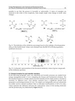
The shape and dimensions of a microstrip resonator centred at 610 MHz are shown in
Fig. 21. The centre frequency can be tuned in a small range by changing the lengths of the
stubs A and B. The resonator is designed on a 0.50 mm thick MgO substrate. More details on
the design of this resonator can be found in the reference (Zhou et al., 2005).
To determine the coupling strength between resonators, the structure shown in Fig. 22(a) is
used for simulation. The couplings between the resonators and the feed lines are much
weaker than that between the two resonators. As discussed in section 0, two resonant
frequencies will be obtained from the simulation as shown in Fig. 22(b), similar to Fig. 16.
The coupling coefficient can be extracted by using equation (39). The coupling coefficient is
a function of the distance d between the resonators, and the relationship between the
coupling strength and the distance d is shown in Fig. 23. It can be found in Fig. 23 that two
resonators with a distance of 0.60 mm have a coupling coefficient 0.0059, which is very close
to the required value of 0.005901.


Fig. 21. Layout of the resonator centred at 610 MHz. The minimum line and gap widths are
0.050 mm. Other detailed dimensions are shown in the figure (unit: mm).


(a) (b)
Fig. 22. (a) The structure to determine the coupling strength between resonators in the
simulation, and (b) the simulated response for d = 0.6 mm.

The external coupling between the end resonator and the termination is realized by a tapped
line, as shown in Fig. 24(a). The length t along the signal line of the resonator, from the

tapped line to the middle of the resonator, controls the strength of the external coupling. The

resonator is weakly coupled to the other feed line, so that the circuit can be regarded as a
singly loaded resonator as discussed in section 0. The wide microstrip line connected to port
1 has a characteristic impedance of 50 ohm, the length of which does not affect the response
of the circuit.
0
0.001
0.002
0.003
0.004
0.005
0.006
0.007
0.008
0.4 1.4 2.4 3.4 4.4 5.4 6.4
Distance (d) between resonators (mm)
Coupling coefficient

Fig. 23. The coupling coefficient against the distance between the resonators.

The simulated response is shown in Fig. 24(b), similar to Fig. 18, and the external quality
factor can be extracted by using equation (53). The relationship between the external quality
factor and the length t is shown in Fig. 25. It can be found that t = 4.2 mm gives an external
Q of 135, which is close to the required value of 136.5.


(a) (b)
Fig. 24. (a) The structure to determine the external coupling between the end resonator and
the termination in the simulation (unit: mm) and (b) the simulated response for t = 3.9 mm.

0
50
100
150
200
250
300
350
400
450
500
2 2.5 3 3.5 4 4.5 5 5.5
Distance (t) between the external tapped-line and the middle
of the terminal resonator (mm)
External Q

Fig. 25. The external coupling strength against the length from the tapped line to the middle
of the resonator.

It should be noted that the position of the tapped line also affects the centre frequency of the
end resonator. Therefore the dimensions of the end resonator need to be changed slightly to
keep the desired centre frequency. This is done by changing the length of the stubs A and B
as shown in Fig. 24.
MicrowaveFilters 155

Q
e 0,1
= Q
e 3,4
= 136.5

where M
1,2
and M
2,3
are the coupling coefficients between resonators, and Q
e 0,1
and Q
e 3,4
are
the external factors between the end resonators and the terminations (source and load).

6.2 Determination of the couplings by simulation
The shape and dimensions of a microstrip resonator centred at 610 MHz are shown in
Fig. 21. The centre frequency can be tuned in a small range by changing the lengths of the
stubs A and B. The resonator is designed on a 0.50 mm thick MgO substrate. More details on
the design of this resonator can be found in the reference (Zhou et al., 2005).
To determine the coupling strength between resonators, the structure shown in Fig. 22(a) is
used for simulation. The couplings between the resonators and the feed lines are much
weaker than that between the two resonators. As discussed in section 0, two resonant
frequencies will be obtained from the simulation as shown in Fig. 22(b), similar to Fig. 16.
The coupling coefficient can be extracted by using equation (39). The coupling coefficient is
a function of the distance d between the resonators, and the relationship between the
coupling strength and the distance d is shown in Fig. 23. It can be found in Fig. 23 that two
resonators with a distance of 0.60 mm have a coupling coefficient 0.0059, which is very close
to the required value of 0.005901.


Fig. 21. Layout of the resonator centred at 610 MHz. The minimum line and gap widths are
0.050 mm. Other detailed dimensions are shown in the figure (unit: mm).

(a) (b)
Fig. 22. (a) The structure to determine the coupling strength between resonators in the
simulation, and (b) the simulated response for d = 0.6 mm.

The external coupling between the end resonator and the termination is realized by a tapped
line, as shown in Fig. 24(a). The length t along the signal line of the resonator, from the
tapped line to the middle of the resonator, controls the strength of the external coupling. The

resonator is weakly coupled to the other feed line, so that the circuit can be regarded as a
singly loaded resonator as discussed in section 0. The wide microstrip line connected to port
1 has a characteristic impedance of 50 ohm, the length of which does not affect the response
of the circuit.
0
0.001
0.002
0.003
0.004
0.005
0.006
0.007
0.008
0.4 1.4 2.4 3.4 4.4 5.4 6.4
Distance (d) between resonators (mm)
Coupling coefficient

Fig. 23. The coupling coefficient against the distance between the resonators.

The simulated response is shown in Fig. 24(b), similar to Fig. 18, and the external quality

factor can be extracted by using equation (53). The relationship between the external quality
factor and the length t is shown in Fig. 25. It can be found that t = 4.2 mm gives an external
Q of 135, which is close to the required value of 136.5.


(a) (b)
Fig. 24. (a) The structure to determine the external coupling between the end resonator and
the termination in the simulation (unit: mm) and (b) the simulated response for t = 3.9 mm.
0
50
100
150
200
250
300
350
400
450
500
2 2.5 3 3.5 4 4.5 5 5.5
Distance (t) between the external tapped-line and the middle
of the terminal resonator (mm)
External Q

Fig. 25. The external coupling strength against the length from the tapped line to the middle
of the resonator.

It should be noted that the position of the tapped line also affects the centre frequency of the
end resonator. Therefore the dimensions of the end resonator need to be changed slightly to
keep the desired centre frequency. This is done by changing the length of the stubs A and B

as shown in Fig. 24.
MicrowaveandMillimeterWaveTechnologies:
fromPhotonicBandgapDevicestoAntennaandApplications156


Fig. 26 Layout and dimensions of the three-pole Chebyshev filter (unit: mm), where t = 4.3
and d = 0.60 after optimisation. More detailed dimensions of the resonators can be found in
Fig. 21 and Fig. 24(a).

For the required external Q for this filter, the length of A and B is found to be 1.4 mm, which
compares to the length of 1.625 mm in the original resonator shown in Fig. 21.
The filter is formed in a shape as shown in Fig. 26. It will be discussed blow that further
optimization of the filter is required to achieve optimal performance.

6.3 Circuit optimisation and simulated response
The theoretical response of the three-pole Chebyshev filter designed is shown in Fig. 27. The
theoretical response is obtained by calculation using the coupling coefficients given in
equation (63). More details on the calculation are given in Chapter 8 of the reference (Hong
& Lancaster, 2001).

-40
-35
-30
-25
-20
-15
-10
-5
0
600 605 610 615 620

Frequency (MHz)
S21 & S11 (dB)
S11 simulated
S21 simulated
S21 theoretical
S11 theoretical

Fig. 27. The theoretical and simulated responses of the three-pole Chebyshev filter.

The dimensions obtained in section 0 are used by the full-wave simulator Sonnet (Sonnet
Software, 2009). The simulated response of the filter is shown in Fig. 27. However, the
simulated response using these dimensions is close to, but does not meet the theoretical
response very well. Generally, there are two major reasons. One reason is that, in the
simulator, the dimensions of the circuit are “discrete” rather than “continuous”, so that the

required coupling coefficients can usually be realized proximately, rather than precisely.
This is because in the simulator a “cell” is the basic building block of the circuit. Thus any
part of the circuit may be as small as one cell or may be multiple cells long or wide. For
example, a typical circuit drawn in the simulator is shown in Fig. 28, which has a cell size of
0.05 mm
 0.025 mm. The black dots are the grid points. The dimensions of the circuit in the
horizontal direction, such as w and d, can only be the multiple of 0.05 mm; while the
dimensions in the vertical direction, such as h, can only be the multiple of 0.025 mm. If
d = 0.75 mm would give the required performance, in the simulator, only the proximate
value d = 0.5 or 1.0 mm could be used. The dimensions can be more precise if the cell size is
smaller. But, on the other hand, the simulation time increases exponentially as the cell size
decreases.
Another reason is that the unwanted cross couplings, among non-neighbouring resonators
and between input and output ports, are not considered in the design. These cross couplings
cannot be easily determined before the design as they are not independent to other

couplings, and they become much more complicated in a filter having more resonators.
Alternatively, the simulator (Sonnet Software, 2009) has an “optimisation function”, which
can be used to optimise the dimensions of a circuit to get an optimised performance.


Fig. 28. An example circuit drawn in the EM simulator (Sonnet Software, 2009).

By using this function, the user may select dimensions of the circuit and define them as a
parameter. In the analysis, the simulator controls the parameter value, within a user defined
range, in an attempt to reach a user defined goal. More than one parameters can be used
simultaneously in the simulation if necessary. More detailed information about the
optimisation can be found in the reference (Sonnet Software, 2009).
The dimensions of the three-pole filter after optimisation by the simulator are shown in
Fig. 26, where t = 4.3 mm and d = 0.60 mm. The optimised response is shown in Fig. 29,
which agrees very well with the theoretical result. The optimised passband has a ripple of
0.014 dB, very close to the target of 0.01 dB; and the minimum return loss is better than
25 dB in the passband, also close to the theoretical value of 26.3 dB.

-0.02
-0.015
-0.01
-0.005
0
608 608.5 609 609.5 610 610.5 611 611.5 612
Frequency (MHz)
S21 (dB)
S21 optimised
S21 theoretical

(a)

MicrowaveFilters 157


Fig. 26 Layout and dimensions of the three-pole Chebyshev filter (unit: mm), where t = 4.3
and d = 0.60 after optimisation. More detailed dimensions of the resonators can be found in
Fig. 21 and Fig. 24(a).

For the required external Q for this filter, the length of A and B is found to be 1.4 mm, which
compares to the length of 1.625 mm in the original resonator shown in Fig. 21.
The filter is formed in a shape as shown in Fig. 26. It will be discussed blow that further
optimization of the filter is required to achieve optimal performance.

6.3 Circuit optimisation and simulated response
The theoretical response of the three-pole Chebyshev filter designed is shown in Fig. 27. The
theoretical response is obtained by calculation using the coupling coefficients given in
equation (63). More details on the calculation are given in Chapter 8 of the reference (Hong
& Lancaster, 2001).

-40
-35
-30
-25
-20
-15
-10
-5
0
600 605 610 615 620
Frequency (MHz)
S21 & S11 (dB)

S11 simulated
S21 simulated
S21 theoretical
S11 theoretical

Fig. 27. The theoretical and simulated responses of the three-pole Chebyshev filter.

The dimensions obtained in section 0 are used by the full-wave simulator Sonnet (Sonnet
Software, 2009). The simulated response of the filter is shown in Fig. 27. However, the
simulated response using these dimensions is close to, but does not meet the theoretical
response very well. Generally, there are two major reasons. One reason is that, in the
simulator, the dimensions of the circuit are “discrete” rather than “continuous”, so that the

required coupling coefficients can usually be realized proximately, rather than precisely.
This is because in the simulator a “cell” is the basic building block of the circuit. Thus any
part of the circuit may be as small as one cell or may be multiple cells long or wide. For
example, a typical circuit drawn in the simulator is shown in Fig. 28, which has a cell size of
0.05 mm
 0.025 mm. The black dots are the grid points. The dimensions of the circuit in the
horizontal direction, such as w and d, can only be the multiple of 0.05 mm; while the
dimensions in the vertical direction, such as h, can only be the multiple of 0.025 mm. If
d = 0.75 mm would give the required performance, in the simulator, only the proximate
value d = 0.5 or 1.0 mm could be used. The dimensions can be more precise if the cell size is
smaller. But, on the other hand, the simulation time increases exponentially as the cell size
decreases.
Another reason is that the unwanted cross couplings, among non-neighbouring resonators
and between input and output ports, are not considered in the design. These cross couplings
cannot be easily determined before the design as they are not independent to other
couplings, and they become much more complicated in a filter having more resonators.
Alternatively, the simulator (Sonnet Software, 2009) has an “optimisation function”, which

can be used to optimise the dimensions of a circuit to get an optimised performance.


Fig. 28. An example circuit drawn in the EM simulator (Sonnet Software, 2009).

By using this function, the user may select dimensions of the circuit and define them as a
parameter. In the analysis, the simulator controls the parameter value, within a user defined
range, in an attempt to reach a user defined goal. More than one parameters can be used
simultaneously in the simulation if necessary. More detailed information about the
optimisation can be found in the reference (Sonnet Software, 2009).
The dimensions of the three-pole filter after optimisation by the simulator are shown in
Fig. 26, where t = 4.3 mm and d = 0.60 mm. The optimised response is shown in Fig. 29,
which agrees very well with the theoretical result. The optimised passband has a ripple of
0.014 dB, very close to the target of 0.01 dB; and the minimum return loss is better than
25 dB in the passband, also close to the theoretical value of 26.3 dB.

-0.02
-0.015
-0.01
-0.005
0
608 608.5 609 609.5 610 610.5 611 611.5 612
Frequency (MHz)
S21 (dB)
S21 optimised
S21 theoretical

(a)
MicrowaveandMillimeterWaveTechnologies:
fromPhotonicBandgapDevicestoAntennaandApplications158

-40
-35
-30
-25
-20
-15
-10
-5
0
600 605 610 615 620
Frequency (MHz)
S21 & S11 (dB)
S11 optimised
S21 optimised
S21 theoretical
S11 theoretical

(b)
Fig. 29. The theoretical and optimised performances of the 3-pole Chebyshev filter.

7. Summary

The general theory of microwave filter design based on lumped-element circuit is described
in this chapter. The lowpass prototype filters with Butterworth, Chebyshev and quasi-
elliptic characteristics are synthesized, and the prototype filters are then transformed to
bandpass filters by lowpass to bandpass frequency mapping. By using immitance inverters
(
J - or
K

-inverters), the bandpass filters can be realized by the same type of resonators. One
design example is given to verify the theory on how to design microwave filters.

8. Reference

Collin R. E. (2001). Foundation for Microwave Engineering, John Wiley & Sons, Inc. ISBN: ISBN
0-7803-6031-1. New Jersey.
Hong, J. S. & Lancaster, M. J. (2000). Design of Highly Selective Microstrip Bandpass Filters
with a Single Pair of Attenuation Poles at Finite Frequencies, IEEE Transactions on
Microwave Theory and Technology, vol. 48, July 2000. pp. 1098-1107.
Hong, J. S. & Lancaster, M. J. (2001). Microstrip Filters for RF/Microwave Applications, John
Wiley & Sons, INC. ISBN: 0-471-38877-7, New York.
Levy, R. (1976). Filters with single transmission zeros at real and imaginary frequencies, IEEE
Transactions on Microwave Theory and Technology, vol. 24, Apr. 1976. pp. 172-181.
Matthaei, G.; Young, L. & Jones, E.M.T. (1980). Micorwave Filters, Impedance-matching
Networks and Coupling Structure, Artech House, INC. 685 Canton Street, Norwood,
MA 02062.
Rhodes, J. D. (1976). Theory of Electrical Filters, Willey. ISBN: 0-471-71806-8, New York.
Rhodes, J. D. & Alseyab, S. A. (1980). The generalized Chebyshev low-pass prototype filter.
Circuit Theory Application, vol.8, 1980. pp.113-125.
Sonnet Software (2009), EM User’s Manual, Sonnet Software, Inc. Elwood Davis Road North
Syracuse, NY 13212
Zhou, J.; Lancaster, M. J.; Huang, F.; Roddis, N. & Glynn, D. (2005) HTS narrow band filters
at UHF band for radio astronomy applications, IEEE Transactions on Applied
Superconductivity, vol.15, June 2005. pp.1004 – 1007.
RecongurableMicrowaveFilters 159
RecongurableMicrowaveFilters
IgnacioLlamas-GarroandZabdielBrito-Brito
x

Reconfigurable Microwave Filters

Ignacio Llamas-Garro and Zabdiel Brito-Brito
Technical University of Catalonia
Spain

1. Introduction

Reconfigurable microwave filters make microwave transceivers adaptable to multiple bands
of operation using a single filter, which is highly desirable in today’s communications with
evermore growing wireless applications. Tunable filters can replace the necessity of
switching between several filters to have more than one filter response by introducing
tuning elements embedded into a filter topology.
Microwave tunable filters can be divided in two groups, filters with discrete tuning, and
filters with continuous tuning. Filter topologies presenting a discrete tuning generally use
PIN diodes or MEMS switches. On the other hand, filter topologies using varactor diodes,
MEMS capacitors, ferroelectric materials or ferromagnetic materials are frequently used to
obtain a continuous tuning device. Filter topologies can mix continuous and discrete tuning
by combining tuning elements as well, e.g. the use of switches and varactors on a filter
topology can form part of a discrete and continuous tuned device.
Center frequency is the most common filter parameter to reconfigure. Fewer designs
reconfigure other parameters, such as the bandwidth or selectivity. When deciding which
technology is adequate for a given application, the designer must consider the following
issues: cost, power consumption, size, performance and operating frequency. This chapter
intends to provide a broad view of the microwave reconfigurable filters field, where
different technologies used to reconfigure filters are discussed through different chapter
sections, and finally an overall view of the field is given in the conclusions section at the end
of the chapter.
This chapter starts discussing filters that use active devices as tuning elements in section 2;
these include the PIN diode, the varactor diode, the transistor and Monolithic Microwave

Integrated Circuit (MMIC) implementation. Section 3 discusses the use of Micro Electro
Mechanical Systems (MEMS) as tuning elements on filter topologies; the section discusses
the use of MEMS switches and MEMS varactors. Section 4 contains tunable filters using
ferroelectric materials, where devices using the most common ferroelectrics are discussed.
Section 5 contains filters that use ferromagnetic materials as tuning elements, the section
discusses circuits using Yttrium-Iron-Garnet (YIG) films and other ferromagnetic tuning
mechanisms.
Section 6 describes devices that combine some of the technologies discussed in previous
sections to achieve reconfigurable filter parameters. Section 7 contains a discussion of
7
MicrowaveandMillimeterWaveTechnologies:
fromPhotonicBandgapDevicestoAntennaandApplications160

traditional filter tuning techniques using dielectric or metallic mechanically adjustable
tuning screws. Section 8 gives an overall conclusion of this chapter.

2. Tunable filters using active devices

This section covers tunable filters that use semiconductor based tuning elements. Devices
using diodes are attractive below 10 GHz where diodes can still show quality factors above
50 with low bias voltages. Diodes usually involve simple packages and can be mounted on
microwave boards, many of these designs are thought as potential monolithic designs. This
section covers tunable filters that use PIN diodes, varactor diodes, transistors and ends with
a discussion on monolithic designs.

2.1. Tunable filters using PIN diodes
PIN diodes are frequently used to produce reconfigurable discrete states on a filter response,
and are very attractive for low cost implementations. In this section, tunable filters using
PIN diodes are discussed in distributed and lumped topologies as well a design using
periodic structures.

2.1.1. Distributed designs
Recently in (Brito-Brito et al., 2008) the relation between fractional bandwidth and the
reactance slope parameter of switchable decoupling resonators has been discussed. This
technique has been used to implement two switchable bandstop filters (Brito-Brito et al.,
2009 b); these filters can switch between two center frequency states, each having a defined
fractional bandwidth. The filters have been implemented to provide the same fractional
bandwidth at both center frequencies or different bandwidths defined by the shape of
bended switchable resonator extensions, these two topologies are shown in Fig. 1.
The filter presented in (Lugo & Papapolymerou, 2004) can produce broad and narrow
bandwidths by modifying inter-resonator couplings. The filter in (Koochakzadeh &
Abbaspour-Tamijani, 2007) covers a frequency tuning range from 290 to 600 MHz in four
steps using ten PIN diodes.
A tunable side coupled resonator filter with three center frequency states and two possible
bandwidths for each state can be found in (Lugo & Papapolymerou, 2006 a). A
reconfigurable bandpass filter for WiFi and UMTS transmit standards (Brito-Brito et al., 2009
a) is shown in Fig. 2, the filter has been designed to precisely provide the center frequency
and bandwidth required for each application with low loss and low power consumption,
since it only uses two PIN diodes.
The reconfigurable bandpass filter in (Lacombe, 1984) can obtain a pseudo all pass response
or a bandpass response using PIN diodes. A Dual mode resonator filter can be found in
(Lugo & Papapolymerou, 2005), the filter uses a triangular patch resonator to achieve a two
state reconfigurable bandwidth. A reconfigurable bandwidth using a dual mode square
resonator can be found in (Lugo et al., 2005).


(a)

(b)
Fig. 1. Two state switchable bandstop filters using PIN diodes a) constant bandwidth b)

different bandwidth, taken from (Brito-Brito et al., 2009 b).

Other dual mode resonator filter is presented in (Lugo & Papapolymerou, 2006 b), this filter
has an asymmetrical filter response, and can tune its center frequency, and transmission
zero position using a modified square resonator. The filter in (Karim et al., 2008) can switch
from a bandstop to a bandpass response for ultra wideband applications using four PIN
diodes. A tunable non uniform microstrip combline filter with a reconfigurable center
frequency of over an octave in the UHF band can be found in (Koochakzadeh & Abbaspour-
Tamijani, 2008), the filter can maintain a constant bandwidth over the center frequency
tuning range.

2.1.2. Lumped element designs
Lumped element filter designs using PIN diodes include a reconfigurable bandwidth design
at 10 GHz able to switch between a 500 MHz and a 1500 MHz bandwidth (Rauscher, 2003).
The filter presented in (Chen & Wang, 2007) uses low-temperature co-fired ceramic
technology and can switch between two center frequency states.

2.1.3. Filters using periodic structures
The filter in (Karim et al., 2006) switches between a bandstop and a bandpass response using
electromagnetic band gap periodic structures on a coplanar ground plane; the filter is
centered at 7.3 GHz.
RecongurableMicrowaveFilters 161

traditional filter tuning techniques using dielectric or metallic mechanically adjustable
tuning screws. Section 8 gives an overall conclusion of this chapter.

2. Tunable filters using active devices

This section covers tunable filters that use semiconductor based tuning elements. Devices
using diodes are attractive below 10 GHz where diodes can still show quality factors above

50 with low bias voltages. Diodes usually involve simple packages and can be mounted on
microwave boards, many of these designs are thought as potential monolithic designs. This
section covers tunable filters that use PIN diodes, varactor diodes, transistors and ends with
a discussion on monolithic designs.

2.1. Tunable filters using PIN diodes
PIN diodes are frequently used to produce reconfigurable discrete states on a filter response,
and are very attractive for low cost implementations. In this section, tunable filters using
PIN diodes are discussed in distributed and lumped topologies as well a design using
periodic structures.

2.1.1. Distributed designs
Recently in (Brito-Brito et al., 2008) the relation between fractional bandwidth and the
reactance slope parameter of switchable decoupling resonators has been discussed. This
technique has been used to implement two switchable bandstop filters (Brito-Brito et al.,
2009 b); these filters can switch between two center frequency states, each having a defined
fractional bandwidth. The filters have been implemented to provide the same fractional
bandwidth at both center frequencies or different bandwidths defined by the shape of
bended switchable resonator extensions, these two topologies are shown in Fig. 1.
The filter presented in (Lugo & Papapolymerou, 2004) can produce broad and narrow
bandwidths by modifying inter-resonator couplings. The filter in (Koochakzadeh &
Abbaspour-Tamijani, 2007) covers a frequency tuning range from 290 to 600 MHz in four
steps using ten PIN diodes.
A tunable side coupled resonator filter with three center frequency states and two possible
bandwidths for each state can be found in (Lugo & Papapolymerou, 2006 a). A
reconfigurable bandpass filter for WiFi and UMTS transmit standards (Brito-Brito et al., 2009
a) is shown in Fig. 2, the filter has been designed to precisely provide the center frequency
and bandwidth required for each application with low loss and low power consumption,
since it only uses two PIN diodes.
The reconfigurable bandpass filter in (Lacombe, 1984) can obtain a pseudo all pass response

or a bandpass response using PIN diodes. A Dual mode resonator filter can be found in
(Lugo & Papapolymerou, 2005), the filter uses a triangular patch resonator to achieve a two
state reconfigurable bandwidth. A reconfigurable bandwidth using a dual mode square
resonator can be found in (Lugo et al., 2005).


(a)

(b)
Fig. 1. Two state switchable bandstop filters using PIN diodes a) constant bandwidth b)
different bandwidth, taken from (Brito-Brito et al., 2009 b).

Other dual mode resonator filter is presented in (Lugo & Papapolymerou, 2006 b), this filter
has an asymmetrical filter response, and can tune its center frequency, and transmission
zero position using a modified square resonator. The filter in (Karim et al., 2008) can switch
from a bandstop to a bandpass response for ultra wideband applications using four PIN
diodes. A tunable non uniform microstrip combline filter with a reconfigurable center
frequency of over an octave in the UHF band can be found in (Koochakzadeh & Abbaspour-
Tamijani, 2008), the filter can maintain a constant bandwidth over the center frequency
tuning range.

2.1.2. Lumped element designs
Lumped element filter designs using PIN diodes include a reconfigurable bandwidth design
at 10 GHz able to switch between a 500 MHz and a 1500 MHz bandwidth (Rauscher, 2003).
The filter presented in (Chen & Wang, 2007) uses low-temperature co-fired ceramic
technology and can switch between two center frequency states.

2.1.3. Filters using periodic structures
The filter in (Karim et al., 2006) switches between a bandstop and a bandpass response using
electromagnetic band gap periodic structures on a coplanar ground plane; the filter is

centered at 7.3 GHz.
MicrowaveandMillimeterWaveTechnologies:
fromPhotonicBandgapDevicestoAntennaandApplications162


(a)

(b)
Fig. 2. Switchable bandpass filter using PIN diodes a) topology b) filter response, taken from
(Brito-Brito et al., 2009 a).

2.2. Tunable filters using varactor diodes
Varactors are typically used for continuous tuned filters. Varactor diodes use the change in
the depletion layer capacitance of a p-n junction as a function of applied bias voltage.
Varactor tuned devices have been used for high tuning speeds; these devices do not exhibit
hysteresis. Tuning speeds of varactor tuned filters are limited only by the time constant of
the bias circuit. Varactor based tunable filters are mainly distributed designs as covered in
this section.
The filter in (Musoll-Anguiano et al., 2009) can reconfigure center frequency, bandwidth and
selectivity, resulting in a fully adaptable bandstop design. A photograph of this filter is
shown in Fig. 3. The filter response when tuning these three parameters is shown in Fig. 4.
The filter in (Chung et al., 2005) can tune center frequency or bandwidth using a compact
hairpin like resonator. The combline filters in (Hunter & Rhodes, 1982 a), (Hunter & Rhodes,
1982 b), (Sanchez-Renedo et al., 2005) and (Brown & Rebeiz, 2000) use suspended stripline
transmission lines. The first design is a bandpass filter, and the second one is a bandstop
filter. The bandpass design can tune its center frequency showing a good impedance
matching for the different filter states. The third design provides both center frequency and
bandwidth control on a bandpass filter topology. The fourth design is a bandpass filter with
a reconfigurable center frequency, respectively.

(a)

(b)
Fig. 3. Tunable bandstop filter using varactor diodes a) topology b) photography of the
filter, taken from (Musoll-Anguiano et al., 2009).

In (Makimoto & Sagawa, 1986) a tunable bandpass filter using microstrip varactor loaded
ring resonators is demonstrated, the device can reconfigure its center frequency. In (Liang &
Zhu, 2001) a filter mixing combline and hairpin like resonators to achieve transmission zeros
on the sides of the passband is presented, the device can tune its center frequency.

2.3. Tunable filters using PIN and varactor diodes
This section reviews filters which combine PIN and Varactor diodes, this results in filter
topologies with discrete and continuous tuning.
RecongurableMicrowaveFilters 163


(a)

(b)
Fig. 2. Switchable bandpass filter using PIN diodes a) topology b) filter response, taken from
(Brito-Brito et al., 2009 a).

2.2. Tunable filters using varactor diodes
Varactors are typically used for continuous tuned filters. Varactor diodes use the change in
the depletion layer capacitance of a p-n junction as a function of applied bias voltage.
Varactor tuned devices have been used for high tuning speeds; these devices do not exhibit
hysteresis. Tuning speeds of varactor tuned filters are limited only by the time constant of
the bias circuit. Varactor based tunable filters are mainly distributed designs as covered in

this section.
The filter in (Musoll-Anguiano et al., 2009) can reconfigure center frequency, bandwidth and
selectivity, resulting in a fully adaptable bandstop design. A photograph of this filter is
shown in Fig. 3. The filter response when tuning these three parameters is shown in Fig. 4.
The filter in (Chung et al., 2005) can tune center frequency or bandwidth using a compact
hairpin like resonator. The combline filters in (Hunter & Rhodes, 1982 a), (Hunter & Rhodes,
1982 b), (Sanchez-Renedo et al., 2005) and (Brown & Rebeiz, 2000) use suspended stripline
transmission lines. The first design is a bandpass filter, and the second one is a bandstop
filter. The bandpass design can tune its center frequency showing a good impedance
matching for the different filter states. The third design provides both center frequency and
bandwidth control on a bandpass filter topology. The fourth design is a bandpass filter with
a reconfigurable center frequency, respectively.


(a)

(b)
Fig. 3. Tunable bandstop filter using varactor diodes a) topology b) photography of the
filter, taken from (Musoll-Anguiano et al., 2009).

In (Makimoto & Sagawa, 1986) a tunable bandpass filter using microstrip varactor loaded
ring resonators is demonstrated, the device can reconfigure its center frequency. In (Liang &
Zhu, 2001) a filter mixing combline and hairpin like resonators to achieve transmission zeros
on the sides of the passband is presented, the device can tune its center frequency.

2.3. Tunable filters using PIN and varactor diodes
This section reviews filters which combine PIN and Varactor diodes, this results in filter
topologies with discrete and continuous tuning.
MicrowaveandMillimeterWaveTechnologies:
fromPhotonicBandgapDevicestoAntennaandApplications164

(a)

(b)

(c)
Fig. 4. Tunable bandstop filter measured responses according to applied bias voltages a)
center frequency tuning b) bandwidth tuning c) selectivity tuning, taken from (Musoll-
Anguiano et al., 2009).

PIN diodes have been used to vary resonator length for frequency tuning and varactor
diodes to modify the bandwidth at each center frequency state in (Carey-Smith & Warr,
2007). This results in discrete center frequency tuning, and continuous bandwidth tuning.

2.4. Tunable filters using transistors
A gallium arsenide field effect transistor has been used as a tuning element in (Torregrosa-
Penalva et al., 2002), the filter topology and frequency response is shown in Fig. 5; the device
is based on a combline topology and can tune its center frequency.
Center frequency tuning has been achieved on a two pole filter configuration using two
metal semiconductor field effect transistors in (Lin & Itoh, 1992), one transistor is used for
center frequency tuning and the other to provide a negative resistance to the circuit. The
negative resistance technique can raise the resonator unloaded quality factor resulting in an
improved filter response.


(a)

(b)
Fig. 5. Tunable bandpass filter using transistors a) topology b) filter response, taken from

(Torregrosa-Penalva et al., 2002).
RecongurableMicrowaveFilters 165


(a)

(b)

(c)
Fig. 4. Tunable bandstop filter measured responses according to applied bias voltages a)
center frequency tuning b) bandwidth tuning c) selectivity tuning, taken from (Musoll-
Anguiano et al., 2009).

PIN diodes have been used to vary resonator length for frequency tuning and varactor
diodes to modify the bandwidth at each center frequency state in (Carey-Smith & Warr,
2007). This results in discrete center frequency tuning, and continuous bandwidth tuning.

2.4. Tunable filters using transistors
A gallium arsenide field effect transistor has been used as a tuning element in (Torregrosa-
Penalva et al., 2002), the filter topology and frequency response is shown in Fig. 5; the device
is based on a combline topology and can tune its center frequency.
Center frequency tuning has been achieved on a two pole filter configuration using two
metal semiconductor field effect transistors in (Lin & Itoh, 1992), one transistor is used for
center frequency tuning and the other to provide a negative resistance to the circuit. The
negative resistance technique can raise the resonator unloaded quality factor resulting in an
improved filter response.


(a)

(b)
Fig. 5. Tunable bandpass filter using transistors a) topology b) filter response, taken from
(Torregrosa-Penalva et al., 2002).