Geoscience and Remote Sensing, New Achievements Part 11 potx
Bạn đang xem bản rút gọn của tài liệu. Xem và tải ngay bản đầy đủ của tài liệu tại đây (5.65 MB, 35 trang )
Methodsandperformancesformulti-passSARInterferometry 343
independent samples (L)
50
60
70
80
90
100
N=30
f
0
[GHz]
independent samples (L)
2 4 6 8
10
20
30
40
5 mm/year
7 mm/year
9 mm/year
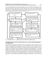
Fig. 3. Number of independent samples to be exploited for each target to get a standard
deviation of the estimate of the subsidence velocity of 5-7-9 mm/year. Frequencies from L to
X band have been exploited.
As a further example, the HCRB allowed us to compute the performances at different fre-
quencies. The number of independent samples to be used to get σ
v
= 5, 7 and 9 mm/year is
plotted in Fig. (3).In computing the HCRB, the temporal decorrelation constant has been up-
dated with the square of the wavelength according to the Markov model in (13), and the APS
phase standard deviation has been updated inversely to the wavelength, the APS delay being
frequency-independent. As a result, the performances drops at the lower frequencies (the L
band), due to the scarce sensitivity of phase to displacements, hence the poor SNR. Likewise,
there is a drop at the high frequencies due to both the temporal and the APS noises. However,
the behavior is flat in the frequencies between S and C band.
4.4.4 Single baseline interferometry
In case of single baseline interferometry, N=2 and there is no way to distinguish between
temporal decorrelation and long term stability. Moreover the phase to be estimated is now a
scalar. Expression (29) leads to the well known CRB (15):
σ
2
φ
=
1 − γ
2
2Lγ
2
4.5 Conclusions
In this chapter a bound for the parametric estimation of the LDF through InSAR has been
discussed. This bound was derived by formulating the problem in such a way as to be han-
dled by the HCRB. This methodology allows for a unified treatment of source decorrelation
(target changes, thermal noise, volumetric effect, etc.) and APS under a consistent statistical
approach. By introducing some reasonable assumptions, we could obtain some closed form
solutions of practical use in InSAR applications. These solutions provide a quick performance
assessment of an InSAR system as a function of its configuration (wavelength, resolution,
SNR), the intrinsic scene decorrelation, and the APS variance. Although some limitations
may arise at higher wavelengths, due to phase wrapping, the result may still be useful for the
design and tuning of the overall system.
5. Phase Linking
The scope of this section is to introduce an algorithm to estimate the set of the interferometric
phases, ϕ
n
, comprehensive of the APS contribution. As discussed in previous chapter, assum-
ing such model is equivalent to retaining phase triangularity, namely ϕ
nm
= ϕ
n
− ϕ
m
. In other
words, we are forcing the problem to be structured in such a way as to explain the phases of
the data covariance matrix simply through N
− 1 real numbers, instead than N(N − 1)/2.
For this reason, the estimated phases will be referred to as Linked Phases, meaning that these
terms are the result of the joint processing of all the N
(N − 1)/2 interferograms. Accordingly,
the algorithm to be described in this section will be referred to as Phase Linking (PL).
An overview of the algorithm is given in the block diagram of Fig. 4. The algorithm is made
of two steps, the first is the phase linking, where the set of N linked phases are optimally
estimated by exploiting the N
(N − 1)/2 interferograms. These phases corresponds to the
optical path, hence ata second step, the APS, the DEM (the target heights) and the deformation
parameters are retrieved.
ML estimate
(linking of Nx(N-1)
interferograms
)
N images
( )
( )
( )
N
j
j
j
φ
φ
φ
exp
exp
exp
ˆ
2
1
=
==
=Φ
ΦΦ
Φ
N-1 estimated phases
APS
& LDF
DEM estimate
& Unwrapping
(
)
( )
( )
N
j
j
j
φ
φ
φ
exp
exp
exp
ˆ
2
1
=
==
=Φ
ΦΦ
Φ
N-1 estimated phases
DEM
APS
LDF
Standard PS-like processor
Fig. 4. Block diagram of the two step algorithm for estimating topography and subsidences.
Before going into details, it is important to note that phase triangularity is automatically sat-
isfied if the data covariance matrix is estimated through a single sample of the data, since
∠
(
y
n
y
∗
m
)
= ∠
(
y
n
)
− ∠
(
y
m
)
. It follows that a necessary condition for the PL algorithm to be
effective is that a suitable estimation window is exploited.
Since the interferometric phases affect the data covariance matrix only through their differ-
ences, one phase (say, n
= 0) will be conventionally used as the reference, in such a way
GeoscienceandRemoteSensing,NewAchievements344
as to estimate the N − 1 phase differences with respect to such reference. Notice that this is
equivalent to estimating N phases under the constraint that ϕ
0
= 0. Therefore, not to add
any further notation, in the following the N
− 1 phase differences will be denoted through
{
ϕ
n
}
N−1
1
. From (7), the log-likelihood function (times −1) is proportional to:
f
ϕ
1
, ϕ
N−1
∝
L
∑
l=1
y
H
(
r
l
, x
l
)
φΓ
−1
φ
H
y
(
r
l
, x
l
)
(37)
∝ trace
φΓ
−1
φ
H
R
where
R is the sample estimate of R or, in other words, it is the matrix of all the available
interferograms averaged over Ω. Rewriting (37), it turns out that the log-likelihood function
may be posed as the following form:
f
ϕ
1
, ϕ
N−1
∝ ξ
H
Γ
−1
◦
R
ξ (38)
where ξ
H
=
1 exp
(
jϕ
1
)
exp
jϕ
N−1
. Hence, the ML estimation of the phases
{
ϕ
n
}
N−1
1
is equivalent to the minimization of the quadratic form of the matrix Γ
−1
◦
R under
the constraint that ξ is a vector of complex exponentials. Unfortunately, we could not find any
closed form solution to this problem, and thus we resorted to an iterative minimization with
respect to each phase, which can be done quite efficiently in closed form:
ϕ
(
k
)
p
= ∠
N
∑
n=p
Γ
−1
np
R
np
exp
j
ϕ
(
k−1
)
n
(39)
where k is the iteration step. The starting point of the iteration was assumed as the phase of
the vector minimizing the quadratic form in (38) under the constraint ξ
0
= 1.
Figures (5 - 7) show the behavior of the variance of the estimates of the N
− 1 phases
{
ϕ
n
}
N−1
1
achieved by running Monte-Carlo simulations with three different scenarios, represented by
the matrices Γ. In order to prove the effectiveness of the PL algorithm, we considered two
phase estimators commonly used in literature. The trivial solution, consisting in evaluating
the phase of the corresponding L-pixel averaged interferograms formed with respect to the
first (n
= 0) image, namely
ϕ
n
= ∠
R
0n
(40)
is named PS-like. The estimator referred to as AR(1) is obtained by evaluating the phases of
the interferograms formed by consecutive acquisitions (i.e. n and n
− 1) and integrating the
result. In formula:
ζ
n
= ∠
R
n,n−1
;
ϕ
n
=
n
∑
k=1
ζ
n
(41)
The name AR(1) was chosen for this phase estimator because it yields the global minimizer
of (38) in the case where the sources decorrelate as an AR(1) process, namely γ
nm
= ρ
|
n−m
|
,
where ρ
∈
(
0, 1
)
. This statement may be easily proved by noticing that if
{
Γ
}
nm
= ρ
|
n−m
|
,
then Γ
−1
is tridiagonal, and thus
ζ
n
, in (41), represents the optimal estimator of the phase
difference ϕ
n
− ϕ
n−1
. In literature this solution has been applied to compensate for temporal
decorrelation in (7), (8), (6), even though in all of these works such choice was made after
heuristical considerations. Finally, the CRB for the phase estimates has been computed by
zeroing the variance of the APSs. In all the simulations it has been exploited an estimation
window as large as 5 independent samples.
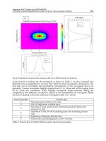
In Fig. (5) it has been assumed a coherence matrix determined by exponential decorrelation.
As stated above, in this case the AR(1) estimator yields the global minimizers of (38), and so
does the PL algorithm, which defaults to this simple solution. The PS-like estimator, instead,
yields significantly worse estimates, due to the progressive loss of coherence induced by the
exponential decorrelation. In Fig. (6) it is considered the case of a constant decorrelation
throughout all of the interferograms. The result provided by the AR(1) estimator is clearly
unacceptable, due to the propagation of the errors caused by the integration step. Conversely,
both the PS-like and the PL estimators produce a stationary phase noise, which is consistent
with the kind of decorrelation used for this simulation. Furthermore, it is interesting to note
that the Linked Phases are less dispersed, proving the effectiveness of the algorithm also in
this simple scenario. Finally, a complex scenario is simulated in Fig. (7) by randomly choosing
the coherence matrix, under the sole constraints that
{
Γ
}
nm
> 0 ∀ n, m and that Γ is positive
definite. As expected, none of the AR(1) and the PS-like estimators is able to handle this
scenario properly, either due to error propagation and coherence losses. In this case, only
through the joint processing of all the interferograms it is possible to retrieve reliable phase
estimates.
Coherence Matrix
0
0.2
0.4
0.6
0.8
1
1 2 3 4 5 6 7 8 9
0
0.5
1
1.5
2
2.5
n
Phase Variance [rad
2
]
PS-like
AR(1)
Phase Linking
CRB
Fig. 5. Variance of the phase estimates. Coherence model:
{
Γ
}
nm
= ρ
|
n−m
|
; ρ = 0.8.
5.1 Phase unwrapping
As stated above, the splitting of the MLE into two steps is advantageous provided that the
two resulting sub-problems are actually easier to solve than the original problem. Despite
we could not find a closed form solution to the PL problem, it must be highlighted that the
algorithm does not require the exploration of the parameter space, thus granting an inter-
esting computational advantage over the one step MLE, especially in the case of a complex
initial parametrization. Instead, difficulties may arise when dealing with the estimation of the
original parameters from the linked phases, since the PL algorithm does not solve for the 2π
ambiguity. As a consequence, a Phase Unwrapping (PU) step is required prior to the moving
to the estimation of the parameters of interest. However, the discussion of a PU technique is
out of the scope of this chapter, we just observe that, once a set of liked phases phases
ϕ
n
has
Methodsandperformancesformulti-passSARInterferometry 345
as to estimate the N − 1 phase differences with respect to such reference. Notice that this is
equivalent to estimating N phases under the constraint that ϕ
0
= 0. Therefore, not to add
any further notation, in the following the N
− 1 phase differences will be denoted through
{
ϕ
n
}
N−1
1
. From (7), the log-likelihood function (times −1) is proportional to:
f
ϕ
1
, ϕ
N−1
∝
L
∑
l=1
y
H
(
r
l
, x
l
)
φΓ
−1
φ
H
y
(
r
l
, x
l
)
(37)
∝ trace
φΓ
−1
φ
H
R
where
R is the sample estimate of R or, in other words, it is the matrix of all the available
interferograms averaged over Ω. Rewriting (37), it turns out that the log-likelihood function
may be posed as the following form:
f
ϕ
1
, ϕ
N−1
∝ ξ
H
Γ
−1
◦
R
ξ (38)
where ξ
H
=
1 exp
(
jϕ
1
)
exp
jϕ
N−1
. Hence, the ML estimation of the phases
{
ϕ
n
}
N−1
1
is equivalent to the minimization of the quadratic form of the matrix Γ
−1
◦
R under
the constraint that ξ is a vector of complex exponentials. Unfortunately, we could not find any
closed form solution to this problem, and thus we resorted to an iterative minimization with
respect to each phase, which can be done quite efficiently in closed form:
ϕ
(
k
)
p
= ∠
N
∑
n=p
Γ
−1
np
R
np
exp
j
ϕ
(
k−1
)
n
(39)
where k is the iteration step. The starting point of the iteration was assumed as the phase of
the vector minimizing the quadratic form in (38) under the constraint ξ
0
= 1.
Figures (5 - 7) show the behavior of the variance of the estimates of the N
− 1 phases
{
ϕ
n
}
N−1
1
achieved by running Monte-Carlo simulations with three different scenarios, represented by
the matrices Γ. In order to prove the effectiveness of the PL algorithm, we considered two
phase estimators commonly used in literature. The trivial solution, consisting in evaluating
the phase of the corresponding L-pixel averaged interferograms formed with respect to the
first (n
= 0) image, namely
ϕ
n
= ∠
R
0n
(40)
is named PS-like. The estimator referred to as AR(1) is obtained by evaluating the phases of
the interferograms formed by consecutive acquisitions (i.e. n and n
− 1) and integrating the
result. In formula:
ζ
n
= ∠
R
n,n−1
;
ϕ
n
=
n
∑
k=1
ζ
n
(41)
The name AR(1) was chosen for this phase estimator because it yields the global minimizer
of (38) in the case where the sources decorrelate as an AR(1) process, namely γ
nm
= ρ
|
n−m
|
,
where ρ
∈
(
0, 1
)
. This statement may be easily proved by noticing that if
{
Γ
}
nm
= ρ
|
n−m
|
,
then Γ
−1
is tridiagonal, and thus
ζ
n
, in (41), represents the optimal estimator of the phase
difference ϕ
n
− ϕ
n−1
. In literature this solution has been applied to compensate for temporal
decorrelation in (7), (8), (6), even though in all of these works such choice was made after
heuristical considerations. Finally, the CRB for the phase estimates has been computed by
zeroing the variance of the APSs. In all the simulations it has been exploited an estimation
window as large as 5 independent samples.
In Fig. (5) it has been assumed a coherence matrix determined by exponential decorrelation.
As stated above, in this case the AR(1) estimator yields the global minimizers of (38), and so
does the PL algorithm, which defaults to this simple solution. The PS-like estimator, instead,
yields significantly worse estimates, due to the progressive loss of coherence induced by the
exponential decorrelation. In Fig. (6) it is considered the case of a constant decorrelation
throughout all of the interferograms. The result provided by the AR(1) estimator is clearly
unacceptable, due to the propagation of the errors caused by the integration step. Conversely,
both the PS-like and the PL estimators produce a stationary phase noise, which is consistent
with the kind of decorrelation used for this simulation. Furthermore, it is interesting to note
that the Linked Phases are less dispersed, proving the effectiveness of the algorithm also in
this simple scenario. Finally, a complex scenario is simulated in Fig. (7) by randomly choosing
the coherence matrix, under the sole constraints that
{
Γ
}
nm
> 0 ∀ n, m and that Γ is positive
definite. As expected, none of the AR(1) and the PS-like estimators is able to handle this
scenario properly, either due to error propagation and coherence losses. In this case, only
through the joint processing of all the interferograms it is possible to retrieve reliable phase
estimates.
Coherence Matrix
0
0.2
0.4
0.6
0.8
1
1 2 3 4 5 6 7 8 9
0
0.5
1
1.5
2
2.5
n
Phase Variance [rad
2
]
PS-like
AR(1)
Phase Linking
CRB
Fig. 5. Variance of the phase estimates. Coherence model:
{
Γ
}
nm
= ρ
|
n−m
|
; ρ = 0.8.
5.1 Phase unwrapping
As stated above, the splitting of the MLE into two steps is advantageous provided that the
two resulting sub-problems are actually easier to solve than the original problem. Despite
we could not find a closed form solution to the PL problem, it must be highlighted that the
algorithm does not require the exploration of the parameter space, thus granting an inter-
esting computational advantage over the one step MLE, especially in the case of a complex
initial parametrization. Instead, difficulties may arise when dealing with the estimation of the
original parameters from the linked phases, since the PL algorithm does not solve for the 2π
ambiguity. As a consequence, a Phase Unwrapping (PU) step is required prior to the moving
to the estimation of the parameters of interest. However, the discussion of a PU technique is
out of the scope of this chapter, we just observe that, once a set of liked phases phases
ϕ
n
has
GeoscienceandRemoteSensing,NewAchievements346
Coherence Matrix
0
0.2
0.4
0.6
0.8
1
n
PS-like
AR(1)
Phase Linking
CRB
Phase Variance [rad
2
]
1 2 3 4 5 6 7 8 9
0
0.2
0.4
0.6
0.8
1
Fig. 6. Variance of the phase estimates. Coherence model:
{
Γ
}
nm
= γ
0
+
(
1 − γ
0
)
δ
n−m
;
γ
0
= 0.6.
been estimated, we just approach PU as in conventional PS processing, that is quite simple
and well tested (1), (5).
6. Parameter estimation
Once the 2π ambiguity has been solved, the linked phases may be expressed in a simple
fashion by modifying the phase model in (3) in such a way as to include the estimate error
committed in the first step. In formula:
ϕ
= ψ
(
θ
)
+
α + υ (42)
where υ represents the estimate error committed by the PL algorithm or, in other words, the
phase noise due to target decorrelation. After the properties of the MLE, υ is asymptotically
distributed as a zero-mean multivariate normal process, with the same covariance matrix as
the one predicted by the CRB (30). In the case of InSAR, the term "asymptotically" is to be
understood to mean that either the estimation window is large or there is a sufficient number
of high coherence interferometric pairs. If these conditions are met, then it sensible to model
the pdf of υ as:
υ
∼ N
0, lim
ε→0
(
X + εI
N
)
−1
(43)
where the covariance matrix of υ has been determined after (23), by zeroing the contribution
of the APSs. Notice that the limit operation could be easily removed by considering a proper
transformation of the linked phases in (42), as discussed in section 4.2. Nevertheless, we
regard that dealing with non transformed phases provides a more natural exposition of how
parameter estimation is performed, and thus we will retain the phase model in (42).
After the discussion in the previous chapter, the APS may be modeled as a zero-mean stochas-
tic process, highly correlated over space, uncorrelated from one acquisition to the other and,
as a first approximation, normally distributed. This leads to expressing the pdf of the linked
phases in as
ϕ
∼ N
ψ
(
θ
)
, lim
ε→0
(
W
ε
)
Coherence Matrix
0
0.2
0.4
0.6
0.8
1
n
PS-like
AR(1)
Phase Linking
CRB
Phase Variance [rad
2
]
1 2 3 4 5 6 7 8 9
0
0.5
1
1.5
2
2.5
Fig. 7. Variance of the phase estimates. Coherence model: random.
where W
ε
is the covariance matrix of the total phase noise,
W
ε
=
(
X + εI
N
)
−1
+ σ
2
α
I
N
, (44)
and σ
2
α
is the variance of the APS.
In order to provide a closed form solution for the estimation of θ from the linked phase, ϕ,
we will focus on the case where the relation between the terms ψ
(
θ
)
and θ is linear, namely
ψ
(
θ
)
=
Θθ. This passage does not involve any loss of generality, as long as that θ is inter-
preted as the set of weights which represent ψ
(
θ
)
in some basis (such as a polynomial basis).
At this point, the MLE of θ from ϕ may be easily derived by minimizing with respect to θ the
quadratic form:
(
ϕ − Θθ
)
T
W
−1
ε
(
ϕ − Θθ
)
, (45)
which yields the linear estimator
θ
= Qϕ, (46)
where
Q
= lim
ε→0
Θ
T
W
−1
ε
Θ
−1
Θ
T
W
−1
ε
(47)
Therefore, the MLE of θ from ϕ is implemented through a weighted L2 norm fit of the model
ψ
(
θ
)
=
Θθ, and W
−1
ε
may be interpreted as the set of weights which allows to fit the model
accounting for target decorrelation and the APSs. It can be shown that the condition that
Θ
T
XΘ is full rank is sufficient to ensure the finiteness of the matrix Q.
By plugging (47) into (46) it turns out that
θ is an unbiased estimator of θ and that the covari-
ance matrix of the estimates is given by:
E
θ
− θ
θ
− θ
T
= QW
ε
Q
T
(48)
= lim
ε→0
Θ
T
(
X + εI
)
−1
+ σ
2
α
I
−1
Θ
−1
Methodsandperformancesformulti-passSARInterferometry 347
Coherence Matrix
0
0.2
0.4
0.6
0.8
1
n
PS-like
AR(1)
Phase Linking
CRB
Phase Variance [rad
2
]
1 2 3 4 5 6 7 8 9
0
0.2
0.4
0.6
0.8
1
Fig. 6. Variance of the phase estimates. Coherence model:
{
Γ
}
nm
= γ
0
+
(
1 − γ
0
)
δ
n−m
;
γ
0
= 0.6.
been estimated, we just approach PU as in conventional PS processing, that is quite simple
and well tested (1), (5).
6. Parameter estimation
Once the 2π ambiguity has been solved, the linked phases may be expressed in a simple
fashion by modifying the phase model in (3) in such a way as to include the estimate error
committed in the first step. In formula:
ϕ
= ψ
(
θ
)
+
α + υ (42)
where υ represents the estimate error committed by the PL algorithm or, in other words, the
phase noise due to target decorrelation. After the properties of the MLE, υ is asymptotically
distributed as a zero-mean multivariate normal process, with the same covariance matrix as
the one predicted by the CRB (30). In the case of InSAR, the term "asymptotically" is to be
understood to mean that either the estimation window is large or there is a sufficient number
of high coherence interferometric pairs. If these conditions are met, then it sensible to model
the pdf of υ as:
υ
∼ N
0, lim
ε→0
(
X + εI
N
)
−1
(43)
where the covariance matrix of υ has been determined after (23), by zeroing the contribution
of the APSs. Notice that the limit operation could be easily removed by considering a proper
transformation of the linked phases in (42), as discussed in section 4.2. Nevertheless, we
regard that dealing with non transformed phases provides a more natural exposition of how
parameter estimation is performed, and thus we will retain the phase model in (42).
After the discussion in the previous chapter, the APS may be modeled as a zero-mean stochas-
tic process, highly correlated over space, uncorrelated from one acquisition to the other and,
as a first approximation, normally distributed. This leads to expressing the pdf of the linked
phases in as
ϕ
∼ N
ψ
(
θ
)
, lim
ε→0
(
W
ε
)
Coherence Matrix
0
0.2
0.4
0.6
0.8
1
n
PS-like
AR(1)
Phase Linking
CRB
Phase Variance [rad
2
]
1 2 3 4 5 6 7 8 9
0
0.5
1
1.5
2
2.5
Fig. 7. Variance of the phase estimates. Coherence model: random.
where W
ε
is the covariance matrix of the total phase noise,
W
ε
=
(
X + εI
N
)
−1
+ σ
2
α
I
N
, (44)
and σ
2
α
is the variance of the APS.
In order to provide a closed form solution for the estimation of θ from the linked phase, ϕ,
we will focus on the case where the relation between the terms ψ
(
θ
)
and θ is linear, namely
ψ
(
θ
)
=
Θθ. This passage does not involve any loss of generality, as long as that θ is inter-
preted as the set of weights which represent ψ
(
θ
)
in some basis (such as a polynomial basis).
At this point, the MLE of θ from ϕ may be easily derived by minimizing with respect to θ the
quadratic form:
(
ϕ − Θθ
)
T
W
−1
ε
(
ϕ − Θθ
)
, (45)
which yields the linear estimator
θ
= Qϕ, (46)
where
Q
= lim
ε→0
Θ
T
W
−1
ε
Θ
−1
Θ
T
W
−1
ε
(47)
Therefore, the MLE of θ from ϕ is implemented through a weighted L2 norm fit of the model
ψ
(
θ
)
=
Θθ, and W
−1
ε
may be interpreted as the set of weights which allows to fit the model
accounting for target decorrelation and the APSs. It can be shown that the condition that
Θ
T
XΘ is full rank is sufficient to ensure the finiteness of the matrix Q.
By plugging (47) into (46) it turns out that
θ is an unbiased estimator of θ and that the covari-
ance matrix of the estimates is given by:
E
θ
− θ
θ
− θ
T
= QW
ε
Q
T
(48)
= lim
ε→0
Θ
T
(
X + εI
)
−1
+ σ
2
α
I
−1
Θ
−1
GeoscienceandRemoteSensing,NewAchievements348
which is the same as (23). The equivalence between (23) and (48) shows that the two step
procedure herein described is asymptotically consistent with the HCRB, and thus it may be
regarded as an optimal solution at sufficiently large signal-to-noise ratios, or when the data
space is large.
It is important to note that the peculiarity of the phase model (42), on which parameter estima-
tion has been based, is constituted by the inclusion of phase noise due to target decorrelation,
represented by υ.In the case where this term is dominated by the APS noise, model (42) would
tends to default to the standard model exploited in PS processing. Accordingly, in this case the
weighted fit carried out by (47) substantially provides the same results as an unweighted fit.
In the framework of InSAR, this is the case where the LDF is to be investigated over distances
larger than the spatial correlation length of the APS. Therefore, the usage of a proper weight-
ing matrix W
−1
ε
is expected to prove its effectiveness in cases where not only the average
displacement of an area is under analysis, but also the local strains.
7. Conditions for the validity of the HCRB for InSAR applications
The equivalence between (23) and (48) provides an alternative methodology to compute the
lower bounds for InSAR performance, through which it is possible to achieve further insights
on the mechanisms that rule the InSAR estimate accuracy. In particular, (48) has been derived
under two hypotheses:
1. the accuracy of the linked phases is close to the CRB;
2. the linked phases can be correctly unwrapped.
As previously discussed, the condition for the validity of hypothesis 1) is that either the esti-
mation window is large or there is a sufficient number of high coherence interferometric pairs.
Approximately, this hypothesis may be considered valid provided that the CRB standard de-
viation of each of the linked phases is much lower than π. Provided that hypothesis 1) is
satisfied, a correct phase unwrapping can be performed provided that both the displacement
field and the APSs are sufficiently smooth functions of the slant range, azimuth coordinates
(15), (31). Accordingly, as far as InSAR applications are concerned, the results predicted by
the HCRB in are meaningful as long as phase unwrapping is not a concern.
8. An experiment on real data
This section is reports an example of application of the two step MLE so far developed. The
data-set available is given by 18 SAR images acquired by ENVISAT
1
over a 4.5 × 4 Km
2
(slant
range, azimuth) area near Las Vegas, US. The scene is characterized by elevations up 600 me-
ters and strong lay-over areas. The normal and temporal baseline spans are about 1400 meters
and 912 days, respectively. The scene is supposed to exhibit a high temporal stability. There-
fore, both temporal decorrelation and the LDF are expected to be negligible. However, many
image pairs are affected by a severe baseline decorrelation. Fig. (8) shows the interferometric
coherence for three image pairs, computed after removing the topographical contributions to
the phase. The first and the third panels (high normal baseline) are characterized by very low
coherence values throughout the whole scene, but for areas in backslope, corresponding to the
bottom right portion of each panel. These panels fully confirm the hypothesis that the scene
1
The SAR sensor aboard ENVISAT operates in C-Band (λ = 5.6 cm) with a resolution of about 9 × 6 m
2
(slant range - azimuth) in the Image mode.
Δt = 79 days
Δb = 1394 m
Δt = 912 days
Δb = 18 m
Δt = 449 days
Δb = 530 m
azimuth [Km]
slant range [Km]
0 1 2 3 4
0
1
2
3
4
azimuth [Km]
0 1 2 3 4
azimuth [Km]
0 1 2 3 4
0
0.2
0.4
0.6
0.8
1
Fig. 8. Scene coherence computed for three image pairs. The coherences have been computed
by exploiting a 3
× 9 pixel window. The topographical contributions to phase have been com-
pensated for by exploiting the estimated DEM.
is to be characterized as being constituted by distributed targets, affected by spatial decorre-
lation. On the other side, the high coherence values in the middle panel (low normal baseline,
high temporal baseline) confirms the hypothesis of a high temporal stability. The aim of this
section is to show the effectiveness of the two step MLE previously depicted by performing a
pixel by pixel estimation of the local topography and the LDF, accounting for the target decor-
relation affecting the data. There are two reasons why the choice of such a data-set is suited
to this goal:
• an a priori information about target statistics, represented by the matrix Γ, is easily
available by using an SRTM DEM;
• the absence of a relevant LDF in the imaged scene represents the best condition to assess
the accuracy.
8.1 Phase Linking and topography estimation
Prior to running the PL algorithm, each SAR image have been demodulated by the interfer-
ometric phase due to topographic contributions, computed by exploiting the SRTM DEM. In
order to avoid problems due to spectral aliasing, each image have been oversampled by a fac-
tor 2 in both the slant range and the azimuth directions. Then the sample covariance matrix
has been computed by averaging all the interferograms over the estimation window, namely:
R
nm
= y
H
n
y
m
(49)
where y
n
is a vector corresponding to the pixels of the n − th image within the estimation
window. The size of the estimation window has been fixed in 3
× 9 pixels (slant range, az-
imuth), corresponding to about 5 independent samples and an imaged area as large as 12
× 20
m
2
in the slant range, azimuth plane.
Methodsandperformancesformulti-passSARInterferometry 349
which is the same as (23). The equivalence between (23) and (48) shows that the two step
procedure herein described is asymptotically consistent with the HCRB, and thus it may be
regarded as an optimal solution at sufficiently large signal-to-noise ratios, or when the data
space is large.
It is important to note that the peculiarity of the phase model (42), on which parameter estima-
tion has been based, is constituted by the inclusion of phase noise due to target decorrelation,
represented by υ.In the case where this term is dominated by the APS noise, model (42) would
tends to default to the standard model exploited in PS processing. Accordingly, in this case the
weighted fit carried out by (47) substantially provides the same results as an unweighted fit.
In the framework of InSAR, this is the case where the LDF is to be investigated over distances
larger than the spatial correlation length of the APS. Therefore, the usage of a proper weight-
ing matrix W
−1
ε
is expected to prove its effectiveness in cases where not only the average
displacement of an area is under analysis, but also the local strains.
7. Conditions for the validity of the HCRB for InSAR applications
The equivalence between (23) and (48) provides an alternative methodology to compute the
lower bounds for InSAR performance, through which it is possible to achieve further insights
on the mechanisms that rule the InSAR estimate accuracy. In particular, (48) has been derived
under two hypotheses:
1. the accuracy of the linked phases is close to the CRB;
2. the linked phases can be correctly unwrapped.
As previously discussed, the condition for the validity of hypothesis 1) is that either the esti-
mation window is large or there is a sufficient number of high coherence interferometric pairs.
Approximately, this hypothesis may be considered valid provided that the CRB standard de-
viation of each of the linked phases is much lower than π. Provided that hypothesis 1) is
satisfied, a correct phase unwrapping can be performed provided that both the displacement
field and the APSs are sufficiently smooth functions of the slant range, azimuth coordinates
(15), (31). Accordingly, as far as InSAR applications are concerned, the results predicted by
the HCRB in are meaningful as long as phase unwrapping is not a concern.
8. An experiment on real data
This section is reports an example of application of the two step MLE so far developed. The
data-set available is given by 18 SAR images acquired by ENVISAT
1
over a 4.5 × 4 Km
2
(slant
range, azimuth) area near Las Vegas, US. The scene is characterized by elevations up 600 me-
ters and strong lay-over areas. The normal and temporal baseline spans are about 1400 meters
and 912 days, respectively. The scene is supposed to exhibit a high temporal stability. There-
fore, both temporal decorrelation and the LDF are expected to be negligible. However, many
image pairs are affected by a severe baseline decorrelation. Fig. (8) shows the interferometric
coherence for three image pairs, computed after removing the topographical contributions to
the phase. The first and the third panels (high normal baseline) are characterized by very low
coherence values throughout the whole scene, but for areas in backslope, corresponding to the
bottom right portion of each panel. These panels fully confirm the hypothesis that the scene
1
The SAR sensor aboard ENVISAT operates in C-Band (λ = 5.6 cm) with a resolution of about 9 × 6 m
2
(slant range - azimuth) in the Image mode.
Δt = 79 days
Δb = 1394 m
Δt = 912 days
Δb = 18 m
Δt = 449 days
Δb = 530 m
azimuth [Km]
slant range [Km]
0 1 2 3 4
0
1
2
3
4
azimuth [Km]
0 1 2 3 4
azimuth [Km]
0 1 2 3 4
0
0.2
0.4
0.6
0.8
1
Fig. 8. Scene coherence computed for three image pairs. The coherences have been computed
by exploiting a 3
× 9 pixel window. The topographical contributions to phase have been com-
pensated for by exploiting the estimated DEM.
is to be characterized as being constituted by distributed targets, affected by spatial decorre-
lation. On the other side, the high coherence values in the middle panel (low normal baseline,
high temporal baseline) confirms the hypothesis of a high temporal stability. The aim of this
section is to show the effectiveness of the two step MLE previously depicted by performing a
pixel by pixel estimation of the local topography and the LDF, accounting for the target decor-
relation affecting the data. There are two reasons why the choice of such a data-set is suited
to this goal:
• an a priori information about target statistics, represented by the matrix Γ, is easily
available by using an SRTM DEM;
• the absence of a relevant LDF in the imaged scene represents the best condition to assess
the accuracy.
8.1 Phase Linking and topography estimation
Prior to running the PL algorithm, each SAR image have been demodulated by the interfer-
ometric phase due to topographic contributions, computed by exploiting the SRTM DEM. In
order to avoid problems due to spectral aliasing, each image have been oversampled by a fac-
tor 2 in both the slant range and the azimuth directions. Then the sample covariance matrix
has been computed by averaging all the interferograms over the estimation window, namely:
R
nm
= y
H
n
y
m
(49)
where y
n
is a vector corresponding to the pixels of the n − th image within the estimation
window. The size of the estimation window has been fixed in 3
× 9 pixels (slant range, az-
imuth), corresponding to about 5 independent samples and an imaged area as large as 12
× 20
m
2
in the slant range, azimuth plane.
GeoscienceandRemoteSensing,NewAchievements350
The PL algorithm has been implemented as shown by equations (38), (39), where the matrix
Γ has been computed at every slant range, azimuth location as a linear combination between
the sample estimate within the estimation window and the a priori information provided by
the SRTM DEM. Then, all the interferograms have been normalized in amplitude, flattened
by the linked phases, and added up, in such a way as to define an index to assess the phase
stability at each slant range, azimuth location. In formula:
Υ
=
∑
nm
y
H
n
y
m
y
n
y
m
exp
(
j
(
ϕ
m
−
ϕ
n
))
(50)
The precise topography has been estimated by plugging the phase stability index defined
in (50) and the linked phases,
ϕ
n
, into a standard PS processors. More explicitly, the phase
stability index has been used as a figure of merit for sampling the phase estimates on a sparse
grid of reliable points, to be used for APS estimation and removal. After removal of the APS,
the residual topography has been estimated on the full grid by means of a Fourier Transform
(1), (5), namely:
q
= arg max
q
∑
n
exp
(
j
(
ϕ
n
− k
z
(
n
)
q
))
(51)
where
q is the topographic error with respect to the SRTM DEM and k
z
(
n
)
is the height to
phase conversion factor for the n
− th image.
The resulting elevation map shows a remarkable improvement in the planimetric and altimet-
ric resolution, see Fig. (9). In order to test the DEM accuracy, the interferograms for three
different image pairs have been formed and compensated for the precise DEM and the APS,
as shown in Fig. (10, top row). Notice that the interferograms decorrelate as the baseline
increases, but for the areas in backslope. In these areas, it is possible to appreciate that the
phases are rather good, showing no relevant residual fringes.
The effectiveness of the Phase Linking algorithm in compensating for spatial decorrelation
phenomena is visible in Fig. (10, bottom row), where the three panels represent the phases
of the same three interferograms as in the top row obtained by computing the (wrapped)
differences among the LPs:
ϕ
nm
=
ϕ
n
−
ϕ
m
. It may be noticed that the estimated phases
exhibit the same fringe patterns as the original interferogram phases, but the phase noise is
significantly reduced, whatever the slope.
This is remarked in Fig. 11, where the histogram of the residual phases of the 1394 m inter-
ferogram (continuous line) is compared to the histogram of the estimated phases of the same
interferogram (dashed line). The width of the central peak may be assessed in about 1 rad,
corresponding to a standard deviation of the elevation of about 1 m.
Finally, Fig. 12 reports the error with respect to the SRTM DEM as estimated by the approach
depicted above (left) and by a conventional PS analysis (right). More precisely, the result in
the right panel has been achieved by substituting the linked phases with the interferogram
phases in (51). Note that APS estimation and removal has been based in both cases on the
linked phases, in such a way as to eliminate the problem of the PS candidate selection in the
PS algorithm. The reason for the discrepancy in the results provided by the Phase Linking
and the PS algorithms is that the data is affected by a severe spatial decorrelation, causing the
Permanent Scatterer model to break down for a large portion of pixels.
Fig. 9. Absolute height map in slant range - azimuth coordinates. Left: elevation map pro-
vided by the SRTM DEM. Right: estimated elevation map
8.2 LDF estimation
A first analysis of the residual fringes (see Fig. 10, middle panels) shows that, as expected,
no relevant displacement occurred during the temporal span of 912 days under analysis. This
result confirms that the residual phases may be mostly attributed to decorrelation noise and to
the residual APSs. Thereafter, all the N
− 1 estimated residual phases have been unwrapped,
in order to estimate the LDF as depicted in section 6. For sake of simplicity, we assumed a
linear subsidence model for each pixel, that is
Θ
=
4π
λ
∆t
1
∆t
2
· · · ∆t
N
T
(52)
being λ the wavelength and ∆t
n
the acquisition time of the n − th image with respect to the
reference image. The weights of the estimator (47) have been derived from the estimates of Γ,
according to (44). As pointed up in section 6, the weighted estimator (47) is expected to prove
its effectiveness over a standard fit (in this case, a linear fitting) in the estimation of local scale
displacements, for which the major source of phase noise is due to target decorrelation. To
this aim, the estimated phases have been selectively high-pass filtered along the slant range,
azimuth plane, in such a way as to remove most of the APS contributions and deal only with
local deformations.
Figure (13) shows the histograms of the estimated LOS velocities obtained by the weighted es-
timator (47) and the standard linear fitting. As expected, the scene does not show any relevant
subsidence and the weighted estimator achieves a lower dispersion of the estimates than the
standard linear fitting. The standard deviation of the estimates of the LOS velocity produced
by the weighted estimator (47) may be quantified in about 0.5 mm/year, whereas the HCRB
standard deviation for the estimate of the LOS velocity is 0.36 mm/year, basing on the average
scene coherence.
The reliability of the LOS velocity estimates has been assessed by computing the mean square
error between the phase history and the fitted model at every slant range, azimuth location,
see Fig. (14). It is worth noting that among the points exhibiting high reliability, few also
exhibit a velocity value significantly higher that the estimate dispersion.
Methodsandperformancesformulti-passSARInterferometry 351
The PL algorithm has been implemented as shown by equations (38), (39), where the matrix
Γ has been computed at every slant range, azimuth location as a linear combination between
the sample estimate within the estimation window and the a priori information provided by
the SRTM DEM. Then, all the interferograms have been normalized in amplitude, flattened
by the linked phases, and added up, in such a way as to define an index to assess the phase
stability at each slant range, azimuth location. In formula:
Υ
=
∑
nm
y
H
n
y
m
y
n
y
m
exp
(
j
(
ϕ
m
−
ϕ
n
))
(50)
The precise topography has been estimated by plugging the phase stability index defined
in (50) and the linked phases,
ϕ
n
, into a standard PS processors. More explicitly, the phase
stability index has been used as a figure of merit for sampling the phase estimates on a sparse
grid of reliable points, to be used for APS estimation and removal. After removal of the APS,
the residual topography has been estimated on the full grid by means of a Fourier Transform
(1), (5), namely:
q
= arg max
q
∑
n
exp
(
j
(
ϕ
n
− k
z
(
n
)
q
))
(51)
where
q is the topographic error with respect to the SRTM DEM and k
z
(
n
)
is the height to
phase conversion factor for the n
− th image.
The resulting elevation map shows a remarkable improvement in the planimetric and altimet-
ric resolution, see Fig. (9). In order to test the DEM accuracy, the interferograms for three
different image pairs have been formed and compensated for the precise DEM and the APS,
as shown in Fig. (10, top row). Notice that the interferograms decorrelate as the baseline
increases, but for the areas in backslope. In these areas, it is possible to appreciate that the
phases are rather good, showing no relevant residual fringes.
The effectiveness of the Phase Linking algorithm in compensating for spatial decorrelation
phenomena is visible in Fig. (10, bottom row), where the three panels represent the phases
of the same three interferograms as in the top row obtained by computing the (wrapped)
differences among the LPs:
ϕ
nm
=
ϕ
n
−
ϕ
m
. It may be noticed that the estimated phases
exhibit the same fringe patterns as the original interferogram phases, but the phase noise is
significantly reduced, whatever the slope.
This is remarked in Fig. 11, where the histogram of the residual phases of the 1394 m inter-
ferogram (continuous line) is compared to the histogram of the estimated phases of the same
interferogram (dashed line). The width of the central peak may be assessed in about 1 rad,
corresponding to a standard deviation of the elevation of about 1 m.
Finally, Fig. 12 reports the error with respect to the SRTM DEM as estimated by the approach
depicted above (left) and by a conventional PS analysis (right). More precisely, the result in
the right panel has been achieved by substituting the linked phases with the interferogram
phases in (51). Note that APS estimation and removal has been based in both cases on the
linked phases, in such a way as to eliminate the problem of the PS candidate selection in the
PS algorithm. The reason for the discrepancy in the results provided by the Phase Linking
and the PS algorithms is that the data is affected by a severe spatial decorrelation, causing the
Permanent Scatterer model to break down for a large portion of pixels.
Fig. 9. Absolute height map in slant range - azimuth coordinates. Left: elevation map pro-
vided by the SRTM DEM. Right: estimated elevation map
8.2 LDF estimation
A first analysis of the residual fringes (see Fig. 10, middle panels) shows that, as expected,
no relevant displacement occurred during the temporal span of 912 days under analysis. This
result confirms that the residual phases may be mostly attributed to decorrelation noise and to
the residual APSs. Thereafter, all the N
− 1 estimated residual phases have been unwrapped,
in order to estimate the LDF as depicted in section 6. For sake of simplicity, we assumed a
linear subsidence model for each pixel, that is
Θ
=
4π
λ
∆t
1
∆t
2
· · · ∆t
N
T
(52)
being λ the wavelength and ∆t
n
the acquisition time of the n − th image with respect to the
reference image. The weights of the estimator (47) have been derived from the estimates of Γ,
according to (44). As pointed up in section 6, the weighted estimator (47) is expected to prove
its effectiveness over a standard fit (in this case, a linear fitting) in the estimation of local scale
displacements, for which the major source of phase noise is due to target decorrelation. To
this aim, the estimated phases have been selectively high-pass filtered along the slant range,
azimuth plane, in such a way as to remove most of the APS contributions and deal only with
local deformations.
Figure (13) shows the histograms of the estimated LOS velocities obtained by the weighted es-
timator (47) and the standard linear fitting. As expected, the scene does not show any relevant
subsidence and the weighted estimator achieves a lower dispersion of the estimates than the
standard linear fitting. The standard deviation of the estimates of the LOS velocity produced
by the weighted estimator (47) may be quantified in about 0.5 mm/year, whereas the HCRB
standard deviation for the estimate of the LOS velocity is 0.36 mm/year, basing on the average
scene coherence.
The reliability of the LOS velocity estimates has been assessed by computing the mean square
error between the phase history and the fitted model at every slant range, azimuth location,
see Fig. (14). It is worth noting that among the points exhibiting high reliability, few also
exhibit a velocity value significantly higher that the estimate dispersion.
GeoscienceandRemoteSensing,NewAchievements352
Δt = 79 days
Δb = 1394 m
slant range [Km]
0
1
2
3
4
azimuth [Km]
slant range [Km]
0 1 2 3 4
0
1
2
3
4
Δt = 912 days
Δb = 18 m
azimuth [Km]
0 1 2 3 4
Δt = 449 days
Δb = 530 m
Interferogram
Phases
azimuth [Km]
Linked
Phases
0 1 2 3 4
Fig. 10. Top row: wrapped phases of three interferograms after subtracting the estimated
topographical and APS contributions. Each panel has been filtered, in order yield the same
spatial resolution as the estimated interferometric phases (3
× 9 pixel). Bottom row: wrapped
phases of the same three interferograms obtained as the differences of the corresponding LPs,
after subtracting the estimated topographical and APS contributions.
9. Conclusions
This section has provided an analysis of the problems that may arise when performing in-
terferometric analysis over scenes characterized by decorrelating scatterers. This analysis has
been performed mainly from a statistical point of view, in order to design algorithms yield-
ing the lowest variance of the estimates. The PL algorithm has been proposed as a MLE of
the (wrapped) interferometric phases directly from the focused SAR images, capable of com-
-3 -2 -1 0 1 2 3
0
5000
10000
15000
phase [rad]
Histogram
Interferogram Phase
Linked Phase
Fig. 11. Histograms of the phase residuals shown in the top and bottom left panels of Fig. 10,
corresponding to a normal baseline of 1394 m.
0 2 4
0
1
2
3
4
0 2 4
azimuth [Km]
slant range [Km]
azimuth [Km]
-30
-20
-10
0
10
20
30
Topography estimated
from the linked phases
Topography estimated
according to the PS
processing
Fig. 12. Left: topography estimated from the linked phases. Right; topography estimated
according to the PS processing. The color scale ranges from
−30 to 30 meters.
-3 -2 -1 0 1 2 3
0
2
4
6
8
10
x 10
4
LOS velocity [mm/year]
Histogram
standard linear fitting
weighted linear fitting
Fig. 13. Histograms of the estimates of the LOS velocity obtained by a standard linear fitting
and the weighted estimator (47).
pensating the loss of information due to target decorrelation by combining all the available
interferograms. This technique has been proven to be very effective in the case where the
target statistics are at least approximately known, getting close to the CRB even for highly
decorrelated sources. Basing on the asymptotic properties of the statistics of the phase esti-
mates, a second MLE has been proposed to optimally fit an arbitrary LDF model from the
unwrapped estimated phases, taking into account both the phase noise due target decorrela-
tion and the presence of the APSs. The estimates have been to shown to be asymptotically
unbiased and minimum variance.
The concepts presented in this chapter have been experimentally tested on an 18 image data-
set spanning a temporal interval of about 30 months and a total normal baseline of about 1400
m. As a result, a DEM of the scene has been produced with 12
× 20 m
2
spatial resolution and
an elevation dispersion of about 1 m. The dispersion of the LOS subsidence velocity estimate
has been assessed to be about 0.5 mm/year.
Methodsandperformancesformulti-passSARInterferometry 353
Δt = 79 days
Δb = 1394 m
slant range [Km]
0
1
2
3
4
azimuth [Km]
slant range [Km]
0 1 2 3 4
0
1
2
3
4
Δt = 912 days
Δb = 18 m
azimuth [Km]
0 1 2 3 4
Δt = 449 days
Δb = 530 m
Interferogram
Phases
azimuth [Km]
Linked
Phases
0 1 2 3 4
Fig. 10. Top row: wrapped phases of three interferograms after subtracting the estimated
topographical and APS contributions. Each panel has been filtered, in order yield the same
spatial resolution as the estimated interferometric phases (3
× 9 pixel). Bottom row: wrapped
phases of the same three interferograms obtained as the differences of the corresponding LPs,
after subtracting the estimated topographical and APS contributions.
9. Conclusions
This section has provided an analysis of the problems that may arise when performing in-
terferometric analysis over scenes characterized by decorrelating scatterers. This analysis has
been performed mainly from a statistical point of view, in order to design algorithms yield-
ing the lowest variance of the estimates. The PL algorithm has been proposed as a MLE of
the (wrapped) interferometric phases directly from the focused SAR images, capable of com-
-3 -2 -1 0 1 2 3
0
5000
10000
15000
phase [rad]
Histogram
Interferogram Phase
Linked Phase
Fig. 11. Histograms of the phase residuals shown in the top and bottom left panels of Fig. 10,
corresponding to a normal baseline of 1394 m.
0 2 4
0
1
2
3
4
0 2 4
azimuth [Km]
slant range [Km]
azimuth [Km]
-30
-20
-10
0
10
20
30
Topography estimated
from the linked phases
Topography estimated
according to the PS
processing
Fig. 12. Left: topography estimated from the linked phases. Right; topography estimated
according to the PS processing. The color scale ranges from
−30 to 30 meters.
-3 -2 -1 0 1 2 3
0
2
4
6
8
10
x 10
4
LOS velocity [mm/year]
Histogram
standard linear fitting
weighted linear fitting
Fig. 13. Histograms of the estimates of the LOS velocity obtained by a standard linear fitting
and the weighted estimator (47).
pensating the loss of information due to target decorrelation by combining all the available
interferograms. This technique has been proven to be very effective in the case where the
target statistics are at least approximately known, getting close to the CRB even for highly
decorrelated sources. Basing on the asymptotic properties of the statistics of the phase esti-
mates, a second MLE has been proposed to optimally fit an arbitrary LDF model from the
unwrapped estimated phases, taking into account both the phase noise due target decorrela-
tion and the presence of the APSs. The estimates have been to shown to be asymptotically
unbiased and minimum variance.
The concepts presented in this chapter have been experimentally tested on an 18 image data-
set spanning a temporal interval of about 30 months and a total normal baseline of about 1400
m. As a result, a DEM of the scene has been produced with 12
× 20 m
2
spatial resolution and
an elevation dispersion of about 1 m. The dispersion of the LOS subsidence velocity estimate
has been assessed to be about 0.5 mm/year.
GeoscienceandRemoteSensing,NewAchievements354
Mean Square Error [rad
2
]
-600 -400 -200 0 200
-1
0
1
v = -1.07 MSE = 0.08
phase [rad]
Acquisition times [days]
LOS velocity
Mean Square Error
2D histogram
0 5 10
-2
0
2
0
1
60
1000
0
0.5
1
1.5
2
2.5
3
3.5
4
4.5
5
Fig. 14. Right: map of the Mean Square Errors. Top left: 2D histogram of LOS velocities
estimated through weighted linear fitting and Mean Square Errors. Bottom left: phase history
of a selected point (continuous line) and the correspondent fitted LDF model (dashed line).
The location of this point is indicated by a red circle in the right panel.
One critical issue of this approach, common to any ML estimation technique, is the need for
a reliable estimate of the scene coherence for every interferometric pair, required to drive the
algorithms. In the case where target decorrelation is mainly determined by the target spatial
distribution, it has been shown that a viable solution is to exploit the availability of a DEM in
order to provide an initial estimate of the coherences. The case where temporal decorrelation
is dominant is clearly more critical, due to the intrinsic difficulty in foreseeing the temporal
behavior of the targets. Solving this problem requires the exploitation of either a very large
estimation window or, which would be better, of a proper physical modeling of temporal
decorrelation, accounting for Brownian Motion, seasonality effects, and other phenomena.
10. References
[1] A. Ferretti, C. Prati, and F. Rocca, “Permanent scatterers in SAR interferometry,” in Inter-
national Geoscience and Remote Sensing Symposium, Hamburg, Germany, 28 June–2 July 1999,
1999, pp. 1–3.
[2] ——, “Permanent scatterers in SAR interferometry,” IEEE Transactions on Geoscience and
Remote Sensing, vol. 39, no. 1, pp. 8–20, Jan. 2001.
[3] N. Adam, B. M. Kampes, M. Eineder, J. Worawattanamateekul, and M. Kircher, “The de-
velopment of a scientific permanent scatterer system,” in ISPRS Workshop High Resolution
Mapping from Space, Hannover, Germany, 2003, 2003, p. 6 pp.
[4] C. Werner, U. Wegmuller, T. Strozzi, and A. Wiesmann, “Interferometric point target anal-
ysis for deformation mapping,” in International Geoscience and Remote Sensing Symposium,
Toulouse, France, 21–25 July 2003, 2003, pp. 3 pages, cdrom.
[5] A. Ferretti, C. Prati, and F. Rocca, “Nonlinear subsidence rate estimation using perma-
nent scatterers in differential SAR interferometry,” IEEE Transactions on Geoscience and
Remote Sensing, vol. 38, no. 5, pp. 2202–2212, Sep. 2000.
[6] A. Hooper, H. Zebker, P. Segall, and B. Kampes, “A new method for measuring defor-
mation on volcanoes and other non-urban areas using InSAR persistent scatterers,” Geo-
physical Research Letters, vol. 31, pp. L23 611, doi:10.1029/2004GL021 737, Dec. 2004.
[7] R. Hanssen, D. Moisseev, and S. Businger, “Resolving the acquisition ambiguity for at-
mospheric monitoring in multi-pass radar interferometry,” in International Geoscience and
Remote Sensing Symposium, Toulouse, France, 21–25 July 2003, 2003, pp. cdrom, 4 pages.
[8] Y. Fialko, “Interseismic strain accumulation and the earthquake potential on the southern
San Andreas fault system,” Nature, vol. 441, pp. 968–971, Jun. 2006.
[9] P. Berardino, G. Fornaro, R. Lanari, and E. Sansosti, “A new algorithm for surface de-
formation monitoring based on small baseline differential SAR interferograms,” IEEE
Transactions on Geoscience and Remote Sensing, vol. 40, no. 11, pp. 2375–2383, 2002.
[10] P. Berardino, F. Casu, G. Fornaro, R. Lanari, M. Manunta, M. Manzo, and E. Sansosti, “A
quantitative analysis of the SBAS algorithm performance,” International Geoscience and
Remote Sensing Symposium, Anchorage, Alaska, 20–24 September 2004, pp. 3321–3324, 2004.
[11] G. Fornaro, A. Monti Guarnieri, A. Pauciullo, and F. De-Zan, “Maximum liklehood multi-
baseline sar interferometry,” Radar, Sonar and Navigation, IEE Proceedings -, vol. 153, no. 3,
pp. 279–288, June 2006.
[12] A. Ferretti, F. Novali, D. Z. F, C. Prati, and F. Rocca, “Moving from ps to slowly decor-
relating targets: a prospective view„” in European Conference on Synthetic Aperture Radar,
Friedrichshafen, Germany, 2–5 June 2008, 2008, pp. 1–4.
[13] F. Rocca, “Modeling interferogram stacks,” Geoscience and Remote Sensing, IEEE Transac-
tions on, vol. 45, no. 10, pp. 3289–3299, Oct. 2007.
[14] A. Monti Guarnieri and S. Tebaldini, “On the exploitation of target statistics for sar in-
terferometry applications,” Geoscience and Remote Sensing, IEEE Transactions on, vol. 46,
no. 11, pp. 3436–3443, Nov. 2008.
[15] R. Bamler and P. Hartl, “Synthetic aperture radar interferometry,” Inverse Problems,
vol. 14, pp. R1–R54, 1998.
[16] G. Franceschetti and G. Fornaro, “Synthetic aperture radar interferometry,” in Synthetic
Aperture Radar processing, G. Franceschetti and R. Lanari, Eds. CRC Press, 1999, ch. 4,
pp. 167–223.
[17] P. Rosen, S. Hensley, I. R. Joughin, F. K. Li, S. Madsen, E. Rodríguez, and R. Goldstein,
“Synthetic aperture radar interferometry,” Proceedings of the IEEE, vol. 88, no. 3, pp. 333–
382, Mar. 2000.
[18] A. Ferretti, A. Monti Guarnieri, C. Prati, F. Rocca, and D. Massonnet, InSAR Principles:
Guidelines for SAR Interferometry Processing and Interpretation, esa tm-19 feb 2007 ed. ESA,
2007.
[19] R. F. Hanssen, Radar Interferometry: Data Interpretation and Error Analysis. Dordrecht:
Kluwer Academic Publishers, 2001.
Methodsandperformancesformulti-passSARInterferometry 355
Mean Square Error [rad
2
]
-600 -400 -200 0 200
-1
0
1
v = -1.07 MSE = 0.08
phase [rad]
Acquisition times [days]
LOS velocity
Mean Square Error
2D histogram
0 5 10
-2
0
2
0
1
60
1000
0
0.5
1
1.5
2
2.5
3
3.5
4
4.5
5
Fig. 14. Right: map of the Mean Square Errors. Top left: 2D histogram of LOS velocities
estimated through weighted linear fitting and Mean Square Errors. Bottom left: phase history
of a selected point (continuous line) and the correspondent fitted LDF model (dashed line).
The location of this point is indicated by a red circle in the right panel.
One critical issue of this approach, common to any ML estimation technique, is the need for
a reliable estimate of the scene coherence for every interferometric pair, required to drive the
algorithms. In the case where target decorrelation is mainly determined by the target spatial
distribution, it has been shown that a viable solution is to exploit the availability of a DEM in
order to provide an initial estimate of the coherences. The case where temporal decorrelation
is dominant is clearly more critical, due to the intrinsic difficulty in foreseeing the temporal
behavior of the targets. Solving this problem requires the exploitation of either a very large
estimation window or, which would be better, of a proper physical modeling of temporal
decorrelation, accounting for Brownian Motion, seasonality effects, and other phenomena.
10. References
[1] A. Ferretti, C. Prati, and F. Rocca, “Permanent scatterers in SAR interferometry,” in Inter-
national Geoscience and Remote Sensing Symposium, Hamburg, Germany, 28 June–2 July 1999,
1999, pp. 1–3.
[2] ——, “Permanent scatterers in SAR interferometry,” IEEE Transactions on Geoscience and
Remote Sensing, vol. 39, no. 1, pp. 8–20, Jan. 2001.
[3] N. Adam, B. M. Kampes, M. Eineder, J. Worawattanamateekul, and M. Kircher, “The de-
velopment of a scientific permanent scatterer system,” in ISPRS Workshop High Resolution
Mapping from Space, Hannover, Germany, 2003, 2003, p. 6 pp.
[4] C. Werner, U. Wegmuller, T. Strozzi, and A. Wiesmann, “Interferometric point target anal-
ysis for deformation mapping,” in International Geoscience and Remote Sensing Symposium,
Toulouse, France, 21–25 July 2003, 2003, pp. 3 pages, cdrom.
[5] A. Ferretti, C. Prati, and F. Rocca, “Nonlinear subsidence rate estimation using perma-
nent scatterers in differential SAR interferometry,” IEEE Transactions on Geoscience and
Remote Sensing, vol. 38, no. 5, pp. 2202–2212, Sep. 2000.
[6] A. Hooper, H. Zebker, P. Segall, and B. Kampes, “A new method for measuring defor-
mation on volcanoes and other non-urban areas using InSAR persistent scatterers,” Geo-
physical Research Letters, vol. 31, pp. L23 611, doi:10.1029/2004GL021 737, Dec. 2004.
[7] R. Hanssen, D. Moisseev, and S. Businger, “Resolving the acquisition ambiguity for at-
mospheric monitoring in multi-pass radar interferometry,” in International Geoscience and
Remote Sensing Symposium, Toulouse, France, 21–25 July 2003, 2003, pp. cdrom, 4 pages.
[8] Y. Fialko, “Interseismic strain accumulation and the earthquake potential on the southern
San Andreas fault system,” Nature, vol. 441, pp. 968–971, Jun. 2006.
[9] P. Berardino, G. Fornaro, R. Lanari, and E. Sansosti, “A new algorithm for surface de-
formation monitoring based on small baseline differential SAR interferograms,” IEEE
Transactions on Geoscience and Remote Sensing, vol. 40, no. 11, pp. 2375–2383, 2002.
[10] P. Berardino, F. Casu, G. Fornaro, R. Lanari, M. Manunta, M. Manzo, and E. Sansosti, “A
quantitative analysis of the SBAS algorithm performance,” International Geoscience and
Remote Sensing Symposium, Anchorage, Alaska, 20–24 September 2004, pp. 3321–3324, 2004.
[11] G. Fornaro, A. Monti Guarnieri, A. Pauciullo, and F. De-Zan, “Maximum liklehood multi-
baseline sar interferometry,” Radar, Sonar and Navigation, IEE Proceedings -, vol. 153, no. 3,
pp. 279–288, June 2006.
[12] A. Ferretti, F. Novali, D. Z. F, C. Prati, and F. Rocca, “Moving from ps to slowly decor-
relating targets: a prospective view„” in European Conference on Synthetic Aperture Radar,
Friedrichshafen, Germany, 2–5 June 2008, 2008, pp. 1–4.
[13] F. Rocca, “Modeling interferogram stacks,” Geoscience and Remote Sensing, IEEE Transac-
tions on, vol. 45, no. 10, pp. 3289–3299, Oct. 2007.
[14] A. Monti Guarnieri and S. Tebaldini, “On the exploitation of target statistics for sar in-
terferometry applications,” Geoscience and Remote Sensing, IEEE Transactions on, vol. 46,
no. 11, pp. 3436–3443, Nov. 2008.
[15] R. Bamler and P. Hartl, “Synthetic aperture radar interferometry,” Inverse Problems,
vol. 14, pp. R1–R54, 1998.
[16] G. Franceschetti and G. Fornaro, “Synthetic aperture radar interferometry,” in Synthetic
Aperture Radar processing, G. Franceschetti and R. Lanari, Eds. CRC Press, 1999, ch. 4,
pp. 167–223.
[17] P. Rosen, S. Hensley, I. R. Joughin, F. K. Li, S. Madsen, E. Rodríguez, and R. Goldstein,
“Synthetic aperture radar interferometry,” Proceedings of the IEEE, vol. 88, no. 3, pp. 333–
382, Mar. 2000.
[18] A. Ferretti, A. Monti Guarnieri, C. Prati, F. Rocca, and D. Massonnet, InSAR Principles:
Guidelines for SAR Interferometry Processing and Interpretation, esa tm-19 feb 2007 ed. ESA,
2007.
[19] R. F. Hanssen, Radar Interferometry: Data Interpretation and Error Analysis. Dordrecht:
Kluwer Academic Publishers, 2001.
GeoscienceandRemoteSensing,NewAchievements356
[20] ——, Radar Interferometry: Data Interpretation and Error Analysis, 2nd ed. Heidelberg:
Springer Verlag, 2005, in preparation.
[21] J. Muñoz Sabater, R. Hanssen, B. M. Kampes, A. Fusco, and N. Adam, “Physical analysis
of atmospheric delay signal observed in stacked radar interferometric data,” in Interna-
tional Geoscience and Remote Sensing Symposium, Toulouse, France, 21–25 July 2003, 2003,
pp. cdrom, 4 pages.
[22] H. A. Zebker and J. Villasenor, “Decorrelation in interferometric radar echoes,” IEEE
Transactions on Geoscience and Remote Sensing, vol. 30, no. 5, pp. 950–959, Sep. 1992.
[23] V. Pascazio and G. Schirinzi, “Multifrequency insar height reconstruction through max-
imum likelihood estimation of local planes parameters,” Image Processing, IEEE Transac-
tions on, vol. 11, no. 12, pp. 1478–1489, Dec 2002.
[24] F. Gini, F. Lombardini, and M. Montanari, “Layover solution in multibaseline sar in-
terferometry,” Aerospace and Electronic Systems, IEEE Transactions on, vol. 38, no. 4, pp.
1344–1356, Oct 2002.
[25] S. Monti Guarnieri, A; Tebaldini, “Hybrid cramÉr
˝
Urao bounds for crustal displacement
field estimators in sar interferometry,” Signal Processing Letters, IEEE, vol. 14, no. 12, pp.
1012–1015, Dec. 2007.
[26] Y. Rockah and P. Schultheiss, “Array shape calibration using sources in unknown
locations–part ii: Near-field sources and estimator implementation,” Acoustics, Speech
and Signal Processing, IEEE Transactions on, vol. 35, no. 6, pp. 724–735, Jun 1987.
[27] I. Reuven and H. Messer, “A barankin-type lower bound on the estimation error of a
hybrid parameter vector,” IEEE Transactions on Information Theory, vol. 43, no. 3, pp. 1084–
1093, May 1997.
[28] H. L. Van Trees, Optimum array processing, W. Interscience, Ed. New York: John Wiley &
Sons, 2002.
[29] F. Rocca, “Synthetic aperture radar: A new application for wave equation techniques,”
Stanford Exploration Project Report, vol. SEP-56, pp. 167–189, 1987.
[30] A. Papoulis, Probability, Random variables, and stochastic processes, ser. McGraw-Hill series
in Electrical Engineering. New York: McGraw-Hill, 1991.
[31] D. C. Ghiglia and M. D. Pritt, Two-dimensional phase unwrapping: theory, algorithms, and
software. New York: John Wiley & Sons, Inc, 1998.
Integrationofhigh-resolution,ActiveandPassiveRemote
SensinginsupporttoTsunamiPreparednessandContingencyPlanning 357
Integration of high-resolution, Active and Passive Remote Sensing in
supporttoTsunamiPreparednessandContingencyPlanning
FabrizioFerrucci
X
Integration of high-resolution, Active and
Passive Remote Sensing in support to Tsunami
Preparedness and Contingency Planning
Fabrizio Ferrucci
Università della Calabria Italy
1. Introduction
Known from time immemorial to the inhabitants of the Pacific region, tsunamis became
worldwide known with the great Indian Ocean disaster of December 26, 2004, and its toll of
about 234'000 deaths, 14'000 missing and over 2,000,000 displaced persons. Beyond
triggering the international help in managing the immediate post-event, and sustaining
eventual rehabilitation of about 10'000 km
2
of hit coastal areas, the disaster scenario was
intensively focused on by spaceborne remote sensing. The latter, was the only fast and
appropriate mean of collecting updated information in as much as 14 hit countries,
stretching from Indonesia to South Africa across the Indian Ocean.
Short-term, institutional satellite observation response was mostly centered on the
International Charter on Space and Major Disasters, a joint endeavor of 17 public and
private satellite owners worldwide (including the three founding agencies: ESA-European
Space Agency, CNES-Centre National d'Etudes Spatiales, and CCRS-Canadian Center for
Remote Sensing) that provided emergency spaceborne imaging and rapid mapping support
(www.disasterscharter.org/web/charter/activations).
In disaster response, remote sensing information needs are usually restrained to damage
assessment, thus have limited duration. This implies that information must be timely and
timely useable, and be provided with high-to-very high spatial resolution.
Conversely, high temporal resolution - useful in repeated damage assessment across
moderate or long lasting events, as for example storm sequences, earthquake swarms and
volcanic unrests - is generally unnecessary in the tsunami case, where damage presents
large amplitude but is assessed once and for all after the main wavetrain has struck.
A much wider community of institutional and private users of remote sensing information,
in form of special cartography products, and much longer lasting benefits are experienced if
information is used for tsunami flooding risk mapping, impact scenario building and the
inherent contingency planning.
Benefits are intimately connected to the characteristics of tsunamis that occur seldom,
propagate at top speeds close to 200 m/s on deep ocean floors, and can hit in a few hours
areas distant thousands of kilometers from the source. On account of these parameters,
tsunami impact mitigation cannot simply rely upon response.
19
GeoscienceandRemoteSensing,NewAchievements358
In 2004, once the earthquake originating the tsunami was felt, it would have been possible to
give a 2-hour advance impact notice in distant countries as India, Sri Lanka and Maldives.
This did not happen, because a monitoring-and-alert system as the current PTWC-Pacific
Tsunami Warning Center managed by NOAA-National Ocean and Atmosphere
Administration (www.prh.noaa.gov/ptwc/) did not exist yet in the Indian Ocean.
However, since slowest velocities of tsunami waves are much larger than humans can run
for escaping them, in lack of efficient emergency plans to enact immediately, it is clear that
the alert system alone would not have solved the problem.
We can conclude that the risk can be mitigated acting principally on early warnings and
preparedness. The latter is by far the leading issue, as preparedness measures can be
effective even without early warning, whereas early warning is useless without
accompanying measures.
Here, we discuss how a multi-technique, integrated remote sensing approach provides the
essential information to satisfy prevention and response needs in a tsunami prone area,
located in the heart of the theater of the great 2004 Indian Ocean tsunami.
2. Tsunamis and Storm Surges
Tsunamis are liquid gravitational waves that are triggered by sudden displacement of water
bodies by co-seismic seafloor dislocation or underwater landslide mass push/pull. The
speed (celerity) of tsunami waves is
V= tanh 2
2
g
d
(1)
with g the gravity acceleration, d the thickness of the water layer in meters and the
wavelength. If the argument of the hyperbolic tangent is large with d >/2, equation (1)
reduces to
max
V
2
g
(2)
whereas in shallow waters and d </20, equation (1) becomes
min
V
g
d
(3)
On account of the steadily large ratio between wavelength and thickness of the water layer,
the shallow water approximation of equation (3) applies generally.
The main parameter that discriminates tsunamis from swell, is wavelength: wind generated
waves present near-constant wavelengths up to a few hundred meters, and periods between
seconds and tens of seconds.
Conversely, a tsunami wave as in equation (2) travelling in a 4000m thick ocean water layer,
locally reaches 200m/s with periods of 100-120 minutes (or wavelenghts of several hundred
kilometers) and unnoticeable amplitude with respect to wavelength. When approaching the
shore ('shoaling') with velocity dropping below 20 m/s, wavelengths shorten to kilometers,
and wave amplitudes increase (run-up) before penetrating coastal areas.
Outstanding wave heights are obtained as a combination of steep seafloor topographic
gradient, and a short distance from the source. The worst documented such case occurred in
the near field of a M
W
=8.0 earthquake in 1946 at Unimak Island, Alaska, where the Scotch
Cap lighthouse was flushed away by a 35-meter high wave.
Reportedly, wave heights for the great Indian Ocean tsunami of 26
th
December 2004, may
have exceeded 15 m along northern Sumatra coasts (Geist et al., 2007). In Sri Lanka, about
2000 km away from the epicentre of the M
W
=9.2±0.1 earthquake, largest wave heights may
have exceeded 10 m in the East, whereas at least 5000 lives were taken by wavetrains not
higher than 4 m, in the South and the Southwest of the island.
YEAR DAMAGE AREA (SOURCE AREA) SOURCE TYPE CASUALTIES
(approx.)
2004 Eastern and Central Indian Ocean (Sumatra) Earthquake 240000
1991 Bangladesh, Chittagong (category-5 tropical cyclone) Storm surge 138000
1970 Bangladesh (Bhola category-4 tropical cyclone) Storm surge 500000
1908 southern Italy, Messina and Reggio Calabria Earthquake 100000
1896 Honshu (off-Sanriku, Japan) Earthquake 27000
1883 Indonesia, Sunda strait (Krakatau) Volcanic eruption
35000
1868 South America Pacific coasts (Peru-Chile, Arica) Earthquake 70000
1771 Japan, Ryukyu Islands Earthquake 13000
1755 Portugal, Lisbon (Alentejo fault and Carrincho bank) Earthquake 60000
1741 Japan, Oshima and Hokkaido (controversial amplitude) Volcano landslide
2000-15000
Table 1. Top-10 deadly seawater floodings worldwide in the last three Centuries, in inverse
temporal order. Most frequent tsunami triggers relate to earthquakes, either directly (co-
seismic displacement) or indirectly (submarine landslides; Tinti et al., 2005): in terms of
ground floor dislocation alone, earthquake Magnitudes M
w
<7 are not believed to trigger
tsunamis. In tropical areas of strong cyclogenetic activity as the Bay of Bengal and the Gulf
of Mexico, the combination of strong tropical storms and low topographic gradient of
coastal areas, may lead to massive inland penetration of sea waters called 'storm surge'.
With little modifications, the above concepts may consistently apply to storm driven water
surges, or 'storm surges', a threat provided with much higher repeat frequency (yearly) than
tsunamis. Storm surges, typically associated to tropical cyclones, are a near-permanent
elevation of the sealevel for the duration of the event, arising from the combination of
extreme atmospheric pressure drop and push of the associated strong winds. Storm surges
are common in tropical areas worldwide. Storm surges were responsible of the largest, flood
related, mass casualty ever scored (in Bangladesh, Bengal Bay, 1970; ca. 500’000, see Table 1).
In economic terms, the costliest tropical storm surge was that associated to hurricane
Katrina, August 2005, with over 100 Billion USD of direct and indirect losses.
3. Rationale
As stated earlier, operational effectiveness in tsunami impact mitigation requires taking
major preparedness measures to allow exposed populations moving fast to the closest safe
area nearby. This solution may allow avoiding blanket evacuation of tsunami jeopardized
Integrationofhigh-resolution,ActiveandPassiveRemote
SensinginsupporttoTsunamiPreparednessandContingencyPlanning 359
In 2004, once the earthquake originating the tsunami was felt, it would have been possible to
give a 2-hour advance impact notice in distant countries as India, Sri Lanka and Maldives.
This did not happen, because a monitoring-and-alert system as the current PTWC-Pacific
Tsunami Warning Center managed by NOAA-National Ocean and Atmosphere
Administration (www.prh.noaa.gov/ptwc/) did not exist yet in the Indian Ocean.
However, since slowest velocities of tsunami waves are much larger than humans can run
for escaping them, in lack of efficient emergency plans to enact immediately, it is clear that
the alert system alone would not have solved the problem.
We can conclude that the risk can be mitigated acting principally on early warnings and
preparedness. The latter is by far the leading issue, as preparedness measures can be
effective even without early warning, whereas early warning is useless without
accompanying measures.
Here, we discuss how a multi-technique, integrated remote sensing approach provides the
essential information to satisfy prevention and response needs in a tsunami prone area,
located in the heart of the theater of the great 2004 Indian Ocean tsunami.
2. Tsunamis and Storm Surges
Tsunamis are liquid gravitational waves that are triggered by sudden displacement of water
bodies by co-seismic seafloor dislocation or underwater landslide mass push/pull. The
speed (celerity) of tsunami waves is
V= tanh 2
2
g
d
(1)
with g the gravity acceleration, d the thickness of the water layer in meters and the
wavelength. If the argument of the hyperbolic tangent is large with d >/2, equation (1)
reduces to
max
V
2
g
(2)
whereas in shallow waters and d </20, equation (1) becomes
min
V
g
d
(3)
On account of the steadily large ratio between wavelength and thickness of the water layer,
the shallow water approximation of equation (3) applies generally.
The main parameter that discriminates tsunamis from swell, is wavelength: wind generated
waves present near-constant wavelengths up to a few hundred meters, and periods between
seconds and tens of seconds.
Conversely, a tsunami wave as in equation (2) travelling in a 4000m thick ocean water layer,
locally reaches 200m/s with periods of 100-120 minutes (or wavelenghts of several hundred
kilometers) and unnoticeable amplitude with respect to wavelength. When approaching the
shore ('shoaling') with velocity dropping below 20 m/s, wavelengths shorten to kilometers,
and wave amplitudes increase (run-up) before penetrating coastal areas.
Outstanding wave heights are obtained as a combination of steep seafloor topographic
gradient, and a short distance from the source. The worst documented such case occurred in
the near field of a M
W
=8.0 earthquake in 1946 at Unimak Island, Alaska, where the Scotch
Cap lighthouse was flushed away by a 35-meter high wave.
Reportedly, wave heights for the great Indian Ocean tsunami of 26
th
December 2004, may
have exceeded 15 m along northern Sumatra coasts (Geist et al., 2007). In Sri Lanka, about
2000 km away from the epicentre of the M
W
=9.2±0.1 earthquake, largest wave heights may
have exceeded 10 m in the East, whereas at least 5000 lives were taken by wavetrains not
higher than 4 m, in the South and the Southwest of the island.
YEAR DAMAGE AREA (SOURCE AREA) SOURCE TYPE CASUALTIES
(approx.)
2004 Eastern and Central Indian Ocean (Sumatra) Earthquake 240000
1991 Bangladesh, Chittagong (category-5 tropical cyclone) Storm surge 138000
1970 Bangladesh (Bhola category-4 tropical cyclone) Storm surge 500000
1908 southern Italy, Messina and Reggio Calabria Earthquake 100000
1896 Honshu (off-Sanriku, Japan) Earthquake 27000
1883 Indonesia, Sunda strait (Krakatau) Volcanic eruption
35000
1868 South America Pacific coasts (Peru-Chile, Arica) Earthquake 70000
1771 Japan, Ryukyu Islands Earthquake 13000
1755 Portugal, Lisbon (Alentejo fault and Carrincho bank) Earthquake 60000
1741 Japan, Oshima and Hokkaido (controversial amplitude) Volcano landslide
2000-15000
Table 1. Top-10 deadly seawater floodings worldwide in the last three Centuries, in inverse
temporal order. Most frequent tsunami triggers relate to earthquakes, either directly (co-
seismic displacement) or indirectly (submarine landslides; Tinti et al., 2005): in terms of
ground floor dislocation alone, earthquake Magnitudes M
w
<7 are not believed to trigger
tsunamis. In tropical areas of strong cyclogenetic activity as the Bay of Bengal and the Gulf
of Mexico, the combination of strong tropical storms and low topographic gradient of
coastal areas, may lead to massive inland penetration of sea waters called 'storm surge'.
With little modifications, the above concepts may consistently apply to storm driven water
surges, or 'storm surges', a threat provided with much higher repeat frequency (yearly) than
tsunamis. Storm surges, typically associated to tropical cyclones, are a near-permanent
elevation of the sealevel for the duration of the event, arising from the combination of
extreme atmospheric pressure drop and push of the associated strong winds. Storm surges
are common in tropical areas worldwide. Storm surges were responsible of the largest, flood
related, mass casualty ever scored (in Bangladesh, Bengal Bay, 1970; ca. 500’000, see Table 1).
In economic terms, the costliest tropical storm surge was that associated to hurricane
Katrina, August 2005, with over 100 Billion USD of direct and indirect losses.
3. Rationale
As stated earlier, operational effectiveness in tsunami impact mitigation requires taking
major preparedness measures to allow exposed populations moving fast to the closest safe
area nearby. This solution may allow avoiding blanket evacuation of tsunami jeopardized
GeoscienceandRemoteSensing,NewAchievements360
areas, that may imply permanent activity banning in large, critical portions of the territory,
especially if the topografic gradient is very low (as in Sri Lanka and Bangladesh, e.g.) and
small increase of water levels lead to deep inland flooding.
In terms of preparedness, this means that escape way solutions must be addressed well in
advance. Considering that unnoticeably elevated areas close to the shoreline can be good,
and sometimes unexpected escape places to single out, map and include in emergency
plans, protection against tsunamis and timeliness of response require the advance drawing
of quantitative impact scenarios.
Emergency cartography must be frequently updated to mirror the modifications with time
in location and value of vulnerable elements (inhabitants, buildings and infrastructures).
This calls for the use of fast, synoptic and high-to-very high resolution mapping
technologies: a need that can be satisfied by airborne and spaceborne remote sensing only.
These concepts drove the design and the carrying out in 2006 - upon request of the
Government of Sri Lanka to the Italian Government - of a thorough field investigation
aimed to ease, provide with quantitative grounds and speed-up the national emergency
planning in tsunami-prone areas. The request addressed the need of drawing a realistic set
of flooding scenarios for most of the coastal areas of the island, with special emphasis on
settlements and infrastructures in the reach of a model tsunami or a model storm surge. The
basic criteria of investigation were broadly inspired by the format of early risk assessment
and scenario simulation in the reference cases of Northwest USA (Mendocino and
Humboldt in northern California, Tacoma in Washington, e.g.).
This portion of the Pacific coast is subjected to frequent tsunami impact from local seismic
sources in the unresting, undersea Mendocino fault zone (Oppenheimer et al., 1993), and is
focused on by the US National Tsunami Hazard Mitigation Program (Lander et al., 1993;
Eisner et al., 2001; Priest et al., 2001; Venturato et al., 2007).
Downstream to US NTHMP, US Geological Survey provided dissemination of impact maps,
portraying different scenarios based on possible tsunami impacts heights, and listing the
number of people that would be affected by tsunamis of 5m, 10m, and 15m height
respectively, with elevation data based on the SRTM (Shuttle Radar Topography Mission)
Digital Elevation Model. The latter, is available worldwide. It displays planimetric
resolution of 90 meters and absolute vertical accuracy of 9.6m (mission specifications). In the
case of Sri Lanka, these parameters were considered not sufficient for reaching the required
level of horizontal and vertical resolution compatible with a terrain heterogeneous at all
scales, densely vegetated, provided with scattered manufacts eventually hidden or partly
covered by tropical vegetation, and displaying negligible topographic gradients as low as 1-
2% over much of the coastal zones of interest.
The drawing of quantitative flooding scenarios required collecting the information needed
for completing the following steps, at the suitable scale:
i) model tsunami (at sea, before impact): requires detailed 3D knowledge of the seabed,
aimed to model and forecast, spot by spot, the wavetrain pattern, the energy distribution
and the run-up before impact. On account of the expected wavelengths to deal with, the
ideal working scale for accurate modelling was considered to lie between 1/10000 and
1/20000 within at least 10 km from the shoreline. In lack of such information, and on
account of unfavorable time and cost implications of an ad-hoc campaign, it was decided to
rely upon the existing, loose seafloor cartographies by NOAA and British Admiralty, and
the few wave heights observed in December 2004 (Liu et al., 2005).
ii) Model flooding (on land, after impact): requires very high-resolution 3-D terrain model,
to simulate the hydraulic behavior of flooded zones at scales of 1/5000 or better, and to
draw the limits of the impact zone, the expected severity of the areal impacts and, if
appropriate, the energy absorption on impacted manufacts. In brief, the risk model and the
scenarios, to permit emergency deciders to plan evacuation and safety measures, and urban
planners to adopt structural measures finalized to ease citizens' escape in case of alert.
According to urban planners, this target requires ground resolutions in the order of 1 m, and
elevation precisions in the order of 0.2+0.3 m to be achieved uniformly over large areas.
Since the 2004 tsunami losses concentrated in ocean-bound strips of variable width, up to
observed maxima of as much as 8 km in the East of the island (Batticaloa), the width of
coastal areas to map and model was fixed at 3 km in average.
This pointed to an expected 1800 km
2
to map in 3D, in very short times (maximum one
month), and with the resolutions/precisions as above: such target - clearly out of reach for
standard topography missions - could be achieved only with use of State-of-the-Art active
and passive remote sensing techniques.
It was chosen to combine airborne LiDAR and Hyperspectral - for top 3D resolution and
simultaneous confidence qualification of elevation data - and spaceborne RaDAR (Prati et
al., 1994) with multispectral mapping (Hirn & Ferrucci, 2005, 2006), aimed to extend Digital
Elevation Model building and thematic mapping, to the whole of the areas requested by the
Sri Lankan Government via the Disaster Management Center in Colombo. As a good
balance between high resolution needs and feasibility issues, operational costs and security
issues, the inter-Government agreement converged on mapping in 3D and at high-to-very
high resolution, a portion of the coastal areas hosting at least two-thirds of damage and
casualties observed in 2004.
Overall, the island had suffered 34'000 casualties and has experienced - for various reasons -
over 1'100'000 displaced persons, ca. 500'000 of of which directly related to the tsunami
destruction. The percentage of tsunami affected coastal populations ranged from 35% in the
northern coastal districts of Kilinochi, to 80% in the eastern districts of Mullaitivu and 78%
in Ampara, whereas the southern districts of Galle, Matara, and Hambantota displayed
about 20% impact, albeit with scattered pockets of severe damage. The location map and the
survey plan are shown in Figure 1.
4. The HyperDEM campaign
Following establishment of the inter-Government agreement five months after the 2004
tsunami, the operational project "'HyperDEM - The precise Digital Elevation Model of the
coastal areas of Sri Lanka", was launched early in September 2005.
The work was completed in summer 2006 after acquisition of an overall data volume of 2.7
TeraBytes. Upon completion of the work, the End Users - the Disaster Management Center
and the Ministry of Disaster Management and Humanitarian Affairs - were provided with
ca. 2'500 km
2
of Digital Elevation Models of the coastal areas (location maps in Figure 1)
Integrationofhigh-resolution,ActiveandPassiveRemote
SensinginsupporttoTsunamiPreparednessandContingencyPlanning 361
areas, that may imply permanent activity banning in large, critical portions of the territory,
especially if the topografic gradient is very low (as in Sri Lanka and Bangladesh, e.g.) and
small increase of water levels lead to deep inland flooding.
In terms of preparedness, this means that escape way solutions must be addressed well in
advance. Considering that unnoticeably elevated areas close to the shoreline can be good,
and sometimes unexpected escape places to single out, map and include in emergency
plans, protection against tsunamis and timeliness of response require the advance drawing
of quantitative impact scenarios.
Emergency cartography must be frequently updated to mirror the modifications with time
in location and value of vulnerable elements (inhabitants, buildings and infrastructures).
This calls for the use of fast, synoptic and high-to-very high resolution mapping
technologies: a need that can be satisfied by airborne and spaceborne remote sensing only.
These concepts drove the design and the carrying out in 2006 - upon request of the
Government of Sri Lanka to the Italian Government - of a thorough field investigation
aimed to ease, provide with quantitative grounds and speed-up the national emergency
planning in tsunami-prone areas. The request addressed the need of drawing a realistic set
of flooding scenarios for most of the coastal areas of the island, with special emphasis on
settlements and infrastructures in the reach of a model tsunami or a model storm surge. The
basic criteria of investigation were broadly inspired by the format of early risk assessment
and scenario simulation in the reference cases of Northwest USA (Mendocino and
Humboldt in northern California, Tacoma in Washington, e.g.).
This portion of the Pacific coast is subjected to frequent tsunami impact from local seismic
sources in the unresting, undersea Mendocino fault zone (Oppenheimer et al., 1993), and is
focused on by the US National Tsunami Hazard Mitigation Program (Lander et al., 1993;
Eisner et al., 2001; Priest et al., 2001; Venturato et al., 2007).
Downstream to US NTHMP, US Geological Survey provided dissemination of impact maps,
portraying different scenarios based on possible tsunami impacts heights, and listing the
number of people that would be affected by tsunamis of 5m, 10m, and 15m height
respectively, with elevation data based on the SRTM (Shuttle Radar Topography Mission)
Digital Elevation Model. The latter, is available worldwide. It displays planimetric
resolution of 90 meters and absolute vertical accuracy of 9.6m (mission specifications). In the
case of Sri Lanka, these parameters were considered not sufficient for reaching the required
level of horizontal and vertical resolution compatible with a terrain heterogeneous at all
scales, densely vegetated, provided with scattered manufacts eventually hidden or partly
covered by tropical vegetation, and displaying negligible topographic gradients as low as 1-
2% over much of the coastal zones of interest.
The drawing of quantitative flooding scenarios required collecting the information needed
for completing the following steps, at the suitable scale:
i) model tsunami (at sea, before impact): requires detailed 3D knowledge of the seabed,
aimed to model and forecast, spot by spot, the wavetrain pattern, the energy distribution
and the run-up before impact. On account of the expected wavelengths to deal with, the
ideal working scale for accurate modelling was considered to lie between 1/10000 and
1/20000 within at least 10 km from the shoreline. In lack of such information, and on
account of unfavorable time and cost implications of an ad-hoc campaign, it was decided to
rely upon the existing, loose seafloor cartographies by NOAA and British Admiralty, and
the few wave heights observed in December 2004 (Liu et al., 2005).
ii) Model flooding (on land, after impact): requires very high-resolution 3-D terrain model,
to simulate the hydraulic behavior of flooded zones at scales of 1/5000 or better, and to
draw the limits of the impact zone, the expected severity of the areal impacts and, if
appropriate, the energy absorption on impacted manufacts. In brief, the risk model and the
scenarios, to permit emergency deciders to plan evacuation and safety measures, and urban
planners to adopt structural measures finalized to ease citizens' escape in case of alert.
According to urban planners, this target requires ground resolutions in the order of 1 m, and
elevation precisions in the order of 0.2+0.3 m to be achieved uniformly over large areas.
Since the 2004 tsunami losses concentrated in ocean-bound strips of variable width, up to
observed maxima of as much as 8 km in the East of the island (Batticaloa), the width of
coastal areas to map and model was fixed at 3 km in average.
This pointed to an expected 1800 km
2
to map in 3D, in very short times (maximum one
month), and with the resolutions/precisions as above: such target - clearly out of reach for
standard topography missions - could be achieved only with use of State-of-the-Art active
and passive remote sensing techniques.
It was chosen to combine airborne LiDAR and Hyperspectral - for top 3D resolution and
simultaneous confidence qualification of elevation data - and spaceborne RaDAR (Prati et
al., 1994) with multispectral mapping (Hirn & Ferrucci, 2005, 2006), aimed to extend Digital
Elevation Model building and thematic mapping, to the whole of the areas requested by the
Sri Lankan Government via the Disaster Management Center in Colombo. As a good
balance between high resolution needs and feasibility issues, operational costs and security
issues, the inter-Government agreement converged on mapping in 3D and at high-to-very
high resolution, a portion of the coastal areas hosting at least two-thirds of damage and
casualties observed in 2004.
Overall, the island had suffered 34'000 casualties and has experienced - for various reasons -
over 1'100'000 displaced persons, ca. 500'000 of of which directly related to the tsunami
destruction. The percentage of tsunami affected coastal populations ranged from 35% in the
northern coastal districts of Kilinochi, to 80% in the eastern districts of Mullaitivu and 78%
in Ampara, whereas the southern districts of Galle, Matara, and Hambantota displayed
about 20% impact, albeit with scattered pockets of severe damage. The location map and the
survey plan are shown in Figure 1.
4. The HyperDEM campaign
Following establishment of the inter-Government agreement five months after the 2004
tsunami, the operational project "'HyperDEM - The precise Digital Elevation Model of the
coastal areas of Sri Lanka", was launched early in September 2005.
The work was completed in summer 2006 after acquisition of an overall data volume of 2.7
TeraBytes. Upon completion of the work, the End Users - the Disaster Management Center
and the Ministry of Disaster Management and Humanitarian Affairs - were provided with
ca. 2'500 km
2
of Digital Elevation Models of the coastal areas (location maps in Figure 1)
GeoscienceandRemoteSensing,NewAchievements362
Fig. 1. (Left) Location map of areas surveyed by airborne LiDAR, hyperspectral and aerial
photo (red squares) and spaceborne RaDAR (blue open squares). In the former, both Digital
Elevation and Digital Surface Models were obtained at 1m resolution; in the latter, only
DSM, at 30m resolution. (Right) Location of Landsat-7/ETM+ (green) and ERS-1 /ERS-
2/ENVISAT (violet) satellite frames used in HyperDEM. ASTER and QuickBird imagery
was also used for satisfying interpretation needs eventually arisen during processing of the
2.7 TeraByte dataset.
4.1 Airborne campaign
The airborne campaign and the related technical activities, were set up and carried out by
the Istituto Nazionale di Oceanografia e Geofisica Sperimentale-OGS of Trieste, Italy. The
survey, planned for integrated operation and combined acquisition of active and passive
instruments at once, was designed on target ground resolutions of 1 m
2
for LiDAR (Figure 2),
and 4 m
2
for hyperspectral (Figures 3, 4).
Fig. 2. Example of 3D rendering of combined LiDAR (1m planimetric resolution, 0.3 m
precision in elevation on steady reflectors) and digital camera aerial scenery (resolution of
0.2 m). Picture taken over the artificial lake of Angunakolapelessa, north of Hambantota,
south Sri Lanka.
After a long waiting because of a long lasting Autumn Monsoon, the survey was finally
carried out in about one month after move-in of instruments to Colombo, early on February,
2006.
About 1'780 km
2
were LiDAR mapped airborne, at the planimetric resolution of 1 meter and
the elevation precision of 0.3 metres (
Figure 1, left), with the following payloads installed on
the airborne platform, a De Havilland DHC-3 single-propeller "Otter" operated by the Sri
Lankan private operator Air Taxi :
a LiDAR system Optech ALTM 3033. The instrument consisted of a Near Infrared
(A=1064 nm) Laser beam with pulse repetition rate of 33KHz. A scanning mirror directs
the Laser optical pulses across the flight path, providing coverage to either sides of the
flight direction. The forward motion of the aircraft provides coverage in the direction of
flight.
ALTM 3033 incorporates a GPS receiver and an Inertial Measurement Unit (IMU), that
acquires flight attitude data at the frequency of 200 Hz.
Integrationofhigh-resolution,ActiveandPassiveRemote
SensinginsupporttoTsunamiPreparednessandContingencyPlanning 363
Fig. 1. (Left) Location map of areas surveyed by airborne LiDAR, hyperspectral and aerial
photo (red squares) and spaceborne RaDAR (blue open squares). In the former, both Digital
Elevation and Digital Surface Models were obtained at 1m resolution; in the latter, only
DSM, at 30m resolution. (Right) Location of Landsat-7/ETM+ (green) and ERS-1 /ERS-
2/ENVISAT (violet) satellite frames used in HyperDEM. ASTER and QuickBird imagery
was also used for satisfying interpretation needs eventually arisen during processing of the
2.7 TeraByte dataset.
4.1 Airborne campaign
The airborne campaign and the related technical activities, were set up and carried out by
the Istituto Nazionale di Oceanografia e Geofisica Sperimentale-OGS of Trieste, Italy. The
survey, planned for integrated operation and combined acquisition of active and passive
instruments at once, was designed on target ground resolutions of 1 m
2
for LiDAR (Figure 2),
and 4 m
2
for hyperspectral (Figures 3, 4).
Fig. 2. Example of 3D rendering of combined LiDAR (1m planimetric resolution, 0.3 m
precision in elevation on steady reflectors) and digital camera aerial scenery (resolution of
0.2 m). Picture taken over the artificial lake of Angunakolapelessa, north of Hambantota,
south Sri Lanka.
After a long waiting because of a long lasting Autumn Monsoon, the survey was finally
carried out in about one month after move-in of instruments to Colombo, early on February,
2006.
About 1'780 km
2
were LiDAR mapped airborne, at the planimetric resolution of 1 meter and
the elevation precision of 0.3 metres (
Figure 1, left), with the following payloads installed on
the airborne platform, a De Havilland DHC-3 single-propeller "Otter" operated by the Sri
Lankan private operator Air Taxi :
a LiDAR system Optech ALTM 3033. The instrument consisted of a Near Infrared
(A=1064 nm) Laser beam with pulse repetition rate of 33KHz. A scanning mirror directs
the Laser optical pulses across the flight path, providing coverage to either sides of the
flight direction. The forward motion of the aircraft provides coverage in the direction of
flight.
ALTM 3033 incorporates a GPS receiver and an Inertial Measurement Unit (IMU), that
acquires flight attitude data at the frequency of 200 Hz.
GeoscienceandRemoteSensing,NewAchievements364
A hyperspectral radiometer AISA Eagle 1K by the Finnish firm SPECIM. It is a
pushbroom scanner made up of a V-NIR hyperspectral sensor, a GPS/INS Applanix
sensor, and a laptop implemented data acquisition unit.
AISA Eagle 1K operates at wavelengths between 400-970 nm; it is able to record up to 244
bands (with spectral sampling of 2.3 nm/pixel) and 1024 spatial pixels. The system is
flexible enough to allow acquiring data in almost every band combination, simultaneously
acting on the number of bands and the bandwidth by use of a computer assisted procedure.
We operated the system with 42-channel configuration, aimed at improving the signal-noise
ratio in individual spectral bands.
A semi-metric digital camera ROLLEI 6008 db45, with digital back Phase-One, model
H2O. The camera presented a pixel spacing of 9 micrometers, in a scene composed of
4080 x 5440 pixel with 48-bit dynamics. Acquisition is assisted by a camera
compensation system to adjust the roll and pitch variations due to aircraft position and
flight attitude.
The decision to operate simultaneously the semi-metric digital camera with typical footprint
in the order of 0.2 m (when operated at the same flight level useful in obtaining the nominal
LiDAR resolution of 1 m) for assisting in the interpretation of ambiguous elevation features
in the very-high resolution LiDAR and hyperspectral datasets.
In cartography applications, indeed, LiDAR raw elevation data are systematically purged of
false or misleading information as those due to lateral backscattering, multiple scattering,
returns from strongly reflecting physical surfaces, and so forth (Baltsavias, 1999; Kraus &
Pfeifer, 1998).
Such information-cleaning process is performed through a classification process that allows
assigning physical meaning to scatterers provided with variable signal/noise ratios. First
pulses are typically associated to strongly reflecting objects, like trees, wires, roofs and
bridges, whereas later (and weaker) pulses are attributed to returns from "ground" (Kraus &
Pfeifer, 1998).
As stated earlier, the average inland extension of prospected area is about 3 km, with an
isolated maximum of over 10 km in the sensitive area of the artificial basin and the dam of
Angunakolapelessa (Figures 1-left and 2), immediate north of Hambantota in the south.
Airborne LiDAR, orthophotos and hyperspectral data were acquired from February 11
th
and
21
st
, in two legs, separated by a four-day interval (17
th
to 20
th
February) devoted to process
acquired data, assess the dataset completeness and plan eventual recoveries. The flight zone
(Figure 1, left) spanned between Puttalam, in the West, and Pottuvil, in the Southeast. For
security reasons, authorized flight plans did not include the capital, Colombo, nor some
specific damaged coastal zones in the East (Trincomalee, Batticaloa, Ampara). Instead,
eastern areas (Figure 1) were covered by spaceborne RaDAR, and qualified by high
resolution spaceborne multispectral observation (Figure 1, right). Flight heights ranged
between 900-2700 metres, as a function of the desired ground resolution, the morphology
and land-cover of surveyed areas, and the meteorological conditions.
Flight paths were computed in real time by DGPS (differential kinematic GPS), using data
simultaneously acquired by one GPS receiver onboard the aircraft and two, twin-frequency
geodetic GPS receivers Ashtech (mod. Z-Extreme) at the fixed rate of one measurement per
second. Twin-frequency GPS receivers were operated only on the benchmarks of an ad-hoc
geodetic frame created by OGS, starting from a re-calculated benchmark of the Sri Lanka
Survey Department, at the Katunayake International airport, north of Colombo.
Fig. 3. Automated identification and contouring of 4x4 m
2
pixels unprovided with
vegetation, done on AISA hyperspectral V-NIR data by use of a patented method, mutuated
by burn scar analysis (Ferrucci & Hirn, 2005). Processing was conducted on raw data (left),
aimed to prepare and carry out future operations in real-time. In contoured pixels (center),
LiDAR elevation measurement are expected to be precise within the error estimate (±0.15m
averaged over buildings and bare soils). Unlike vegetation, bare rocks, soils and buildings
are the essential constituents of DSMs (see Figure 5) for flooding and tsunami impact
simulation. The Level-2 classification (right) was used for pixel-by-pixel elevation quality
assessment (Figure 4).
All benchmarks of the new geodetic frame were calculated and located on ellipsoids WGS84
and Everest 1830 in the Transverse Mercator projection. Upon completion of the campaign,
the Sri Lanka Survey Dept. was provided with the monographs of newly established
benchmarks.
The best estimate aircraft trajectory (SBET), made up of fixes spaced 0.15 cm in average,
presented rms residual errors < 0.3m, that are compatible with the required precision in
Integrationofhigh-resolution,ActiveandPassiveRemote
SensinginsupporttoTsunamiPreparednessandContingencyPlanning 365
A hyperspectral radiometer AISA Eagle 1K by the Finnish firm SPECIM. It is a
pushbroom scanner made up of a V-NIR hyperspectral sensor, a GPS/INS Applanix
sensor, and a laptop implemented data acquisition unit.
AISA Eagle 1K operates at wavelengths between 400-970 nm; it is able to record up to 244
bands (with spectral sampling of 2.3 nm/pixel) and 1024 spatial pixels. The system is
flexible enough to allow acquiring data in almost every band combination, simultaneously
acting on the number of bands and the bandwidth by use of a computer assisted procedure.
We operated the system with 42-channel configuration, aimed at improving the signal-noise
ratio in individual spectral bands.
A semi-metric digital camera ROLLEI 6008 db45, with digital back Phase-One, model
H2O. The camera presented a pixel spacing of 9 micrometers, in a scene composed of
4080 x 5440 pixel with 48-bit dynamics. Acquisition is assisted by a camera
compensation system to adjust the roll and pitch variations due to aircraft position and
flight attitude.
The decision to operate simultaneously the semi-metric digital camera with typical footprint
in the order of 0.2 m (when operated at the same flight level useful in obtaining the nominal
LiDAR resolution of 1 m) for assisting in the interpretation of ambiguous elevation features
in the very-high resolution LiDAR and hyperspectral datasets.
In cartography applications, indeed, LiDAR raw elevation data are systematically purged of
false or misleading information as those due to lateral backscattering, multiple scattering,
returns from strongly reflecting physical surfaces, and so forth (Baltsavias, 1999; Kraus &
Pfeifer, 1998).
Such information-cleaning process is performed through a classification process that allows
assigning physical meaning to scatterers provided with variable signal/noise ratios. First
pulses are typically associated to strongly reflecting objects, like trees, wires, roofs and
bridges, whereas later (and weaker) pulses are attributed to returns from "ground" (Kraus &
Pfeifer, 1998).
As stated earlier, the average inland extension of prospected area is about 3 km, with an
isolated maximum of over 10 km in the sensitive area of the artificial basin and the dam of
Angunakolapelessa (Figures 1-left and 2), immediate north of Hambantota in the south.
Airborne LiDAR, orthophotos and hyperspectral data were acquired from February 11
th
and
21
st
, in two legs, separated by a four-day interval (17
th
to 20
th
February) devoted to process
acquired data, assess the dataset completeness and plan eventual recoveries. The flight zone
(Figure 1, left) spanned between Puttalam, in the West, and Pottuvil, in the Southeast. For
security reasons, authorized flight plans did not include the capital, Colombo, nor some
specific damaged coastal zones in the East (Trincomalee, Batticaloa, Ampara). Instead,
eastern areas (Figure 1) were covered by spaceborne RaDAR, and qualified by high
resolution spaceborne multispectral observation (Figure 1, right). Flight heights ranged
between 900-2700 metres, as a function of the desired ground resolution, the morphology
and land-cover of surveyed areas, and the meteorological conditions.
Flight paths were computed in real time by DGPS (differential kinematic GPS), using data
simultaneously acquired by one GPS receiver onboard the aircraft and two, twin-frequency
geodetic GPS receivers Ashtech (mod. Z-Extreme) at the fixed rate of one measurement per
second. Twin-frequency GPS receivers were operated only on the benchmarks of an ad-hoc
geodetic frame created by OGS, starting from a re-calculated benchmark of the Sri Lanka
Survey Department, at the Katunayake International airport, north of Colombo.
Fig. 3. Automated identification and contouring of 4x4 m
2
pixels unprovided with
vegetation, done on AISA hyperspectral V-NIR data by use of a patented method, mutuated
by burn scar analysis (Ferrucci & Hirn, 2005). Processing was conducted on raw data (left),
aimed to prepare and carry out future operations in real-time. In contoured pixels (center),
LiDAR elevation measurement are expected to be precise within the error estimate (±0.15m
averaged over buildings and bare soils). Unlike vegetation, bare rocks, soils and buildings
are the essential constituents of DSMs (see Figure 5) for flooding and tsunami impact
simulation. The Level-2 classification (right) was used for pixel-by-pixel elevation quality
assessment (Figure 4).
All benchmarks of the new geodetic frame were calculated and located on ellipsoids WGS84
and Everest 1830 in the Transverse Mercator projection. Upon completion of the campaign,
the Sri Lanka Survey Dept. was provided with the monographs of newly established
benchmarks.
The best estimate aircraft trajectory (SBET), made up of fixes spaced 0.15 cm in average,
presented rms residual errors < 0.3m, that are compatible with the required precision in
GeoscienceandRemoteSensing,NewAchievements366
elevation. Range data were geo-referenced by use of spatial and orientation parameters;
basic products are vectors of points, including the information on position, GPS time and
backscattered LiDAR amplitude. All products were delivered in UTM-44N projection,
WGS84 datum.
Fig. 4. Sample output of the automated identification and contouring process of buildings
and vegetation, done on 56-channel AISA hyperspectral VNIR data by use of a patented
method, mutuated by burn scar analysis (Ferrucci & Hirn, 2005). In these pixels, LiDAR
elevation measurement are expected to be precise within the error estimate (0.15m
averaged over buildings and bare soils).
Finally, bare pixels (without vegetation) were weighted 1, vegetated pixels weighted 0, and
vegetated pixels for which two LiDAR returns are available (an early reflection from the top
of canopy, and a late reflection from the underlying ground) were marked 0.5. This
procedure allowed creating automatically (i) a mask including all points whose elevation is
fully reliable within the nominal error range (Figure 4), and (ii) a three-dimensional, Level-2
land-cover of subsets weighted 0.5 and 1.
The information was completed by carrying out same bare soil classification on
multispectral, very high-resolution, pre-/post-tsunami QuickBird data. In spite of the
comparable pixel footprint, however, the 4-band Visible/Near-Infrared spectral content of
QuickBird provided much poorer information than the airborne 56-band Hyperspectral
airborne radiometer.
LiDAR data were also corrected by use of a geodic model derived from the EGM96 model.
In particular, Digital Elevation Models obtained by airborne LiDAR, were associated to co-
registered airborne Hyperspectral data that underwent unsupervised, Level-2 classification
for automatically discriminating bare soil from vegetation.
Fig. 5. LiDAR-derived Digital Surface Model (DSM, left) and Digital Ground Model (DGM,
right). In the DGM, thick walls are emphasized by removal of most of buildings and
vegetation. Because of such removal, DGMs are suited to standard cartography, but they are
not to tsunami or storm surge flood modelling since they do not contain anymore relevant
obstacles and vulnerable structures. The example relates to the 17
th
Century Dutch fort in
Galle, southern Sri Lanka.
4.2 Spaceborne campaign
The spaceborne campaign was conducted synergetically by the Department of Electronics
and Information of the Politecnico di Milano, that manufactured products in Synthetic
Aperture Radar interferometry with the proprietary procedure PS-InSAR
TM
(Prati et al.,
1994; Ferretti et al., 1999, 2001), and the University of Calabria, that manufactured
multispectral and cartography products exploiting the proprietary procedure MyME2 (Hirn
& Ferrucci, 2005; Ferrucci & Hirn, 2005).
The overall process relied upon same strategy as in the air campaign, with elevation data
founded upon interferometric Synthetic Aperture RaDAR techniques, and pixel
qualification carried out on Infra-Red multispectral satellite scenery.
Pixel qualification was based on the automated discrimination of bare soils, buildings and
infrastructures from vegetation. These classes return highest confidence weight to RaDAR
measured elevation values in the same pixel, whereas dense canopy returns lower or zero
values. Overall, the space dataset was composed of 67 images, both RaDAR and
multispectral, with resolutions ranging from metric (QuickBird) to decametric (ASTER,
Landsat-7, ERS-1, ERS-2, Envisat). To fit the requirements of HyperDEM, repeat-pass
interferometry was carried out to provide for two different products: Permanent Scatterers
Integrationofhigh-resolution,ActiveandPassiveRemote
SensinginsupporttoTsunamiPreparednessandContingencyPlanning 367
elevation. Range data were geo-referenced by use of spatial and orientation parameters;
basic products are vectors of points, including the information on position, GPS time and
backscattered LiDAR amplitude. All products were delivered in UTM-44N projection,
WGS84 datum.
Fig. 4. Sample output of the automated identification and contouring process of buildings
and vegetation, done on 56-channel AISA hyperspectral VNIR data by use of a patented
method, mutuated by burn scar analysis (Ferrucci & Hirn, 2005). In these pixels, LiDAR
elevation measurement are expected to be precise within the error estimate (0.15m
averaged over buildings and bare soils).
Finally, bare pixels (without vegetation) were weighted 1, vegetated pixels weighted 0, and
vegetated pixels for which two LiDAR returns are available (an early reflection from the top
of canopy, and a late reflection from the underlying ground) were marked 0.5. This
procedure allowed creating automatically (i) a mask including all points whose elevation is
fully reliable within the nominal error range (Figure 4), and (ii) a three-dimensional, Level-2
land-cover of subsets weighted 0.5 and 1.
The information was completed by carrying out same bare soil classification on
multispectral, very high-resolution, pre-/post-tsunami QuickBird data. In spite of the
comparable pixel footprint, however, the 4-band Visible/Near-Infrared spectral content of
QuickBird provided much poorer information than the airborne 56-band Hyperspectral
airborne radiometer.
LiDAR data were also corrected by use of a geodic model derived from the EGM96 model.
In particular, Digital Elevation Models obtained by airborne LiDAR, were associated to co-
registered airborne Hyperspectral data that underwent unsupervised, Level-2 classification
for automatically discriminating bare soil from vegetation.
Fig. 5. LiDAR-derived Digital Surface Model (DSM, left) and Digital Ground Model (DGM,
right). In the DGM, thick walls are emphasized by removal of most of buildings and
vegetation. Because of such removal, DGMs are suited to standard cartography, but they are
not to tsunami or storm surge flood modelling since they do not contain anymore relevant
obstacles and vulnerable structures. The example relates to the 17
th
Century Dutch fort in
Galle, southern Sri Lanka.
4.2 Spaceborne campaign
The spaceborne campaign was conducted synergetically by the Department of Electronics
and Information of the Politecnico di Milano, that manufactured products in Synthetic
Aperture Radar interferometry with the proprietary procedure PS-InSAR
TM
(Prati et al.,
1994; Ferretti et al., 1999, 2001), and the University of Calabria, that manufactured
multispectral and cartography products exploiting the proprietary procedure MyME2 (Hirn
& Ferrucci, 2005; Ferrucci & Hirn, 2005).
The overall process relied upon same strategy as in the air campaign, with elevation data
founded upon interferometric Synthetic Aperture RaDAR techniques, and pixel
qualification carried out on Infra-Red multispectral satellite scenery.
Pixel qualification was based on the automated discrimination of bare soils, buildings and
infrastructures from vegetation. These classes return highest confidence weight to RaDAR
measured elevation values in the same pixel, whereas dense canopy returns lower or zero
values. Overall, the space dataset was composed of 67 images, both RaDAR and
multispectral, with resolutions ranging from metric (QuickBird) to decametric (ASTER,
Landsat-7, ERS-1, ERS-2, Envisat). To fit the requirements of HyperDEM, repeat-pass
interferometry was carried out to provide for two different products: Permanent Scatterers