Mobile and wireless communications physical layer development and implementation Part 2 pptx

Bạn đang xem bản rút gọn của tài liệu. Xem và tải ngay bản đầy đủ của tài liệu tại đây (750.54 KB, 20 trang )

WirelessTransmissioninTunnels 11

0
tan ( / 2) /
y y s
k h k h jk h Y (22)

This is an equation for the y-wavenumber and its solution leads to a set of eigenvalues k
yn
,
n=1,2… Now we consider the side walls at x=+w/2. The boundary conditions at these two
walls are

0y s z
E Z H

  (23)

0 y s z
H Y E

  (24)

Using (19) and (21) in (23) leads to a modal equation for k
x
.

0
tan( / 2) /
x

x s
k w k w jk w Z (25)

So (25) is an equation for k
x
whose solution leads to a set of eigenvalues k
xm
. This completes
the modal solution except that we have not satisfied boundary condition (24). Fortunately
however, H
y
is of second order smallness for the lower order modes, hence this boundary
condition can be safely neglected.
Approximate solutions of (22) and (25) for k
yn
and k
xm
in the high frequency regime,
(
0 0
,
s
s
k h Y k w Z  ) are:

0
0
[1 2 / ]
[1 2 / ]
yn s

xm s
k h n j Y k h
k w m j Z k w


 
 
, (26)

where m and n =1,3…are odd integers for the even modes considered. The corresponding
mode attenuation rate is easily obtained as:

2 2 2 3 2 2 2 3
VPmn 0 0
2 Re( ) / 2 Re( ) /
s s
n Y k h m Z k w
  
  Neper/m (27)

The attenuation rate of the corresponding horizontally polarized mode may be obtained
from (27) by exchanging w and h. So:

2 2 2 3 2 2 2 3
0 0
2 Re( ) / 2 Re( ) /
HPmn s s
n Y k w m Z k h
  
  Neper/m (28)

These formulas agree with those derived by Emslie et al (1975). It is worth noting that like
the circular tunnel, the attenuation of the dominant modes is inversely proportional to the
frequency squared and the linear dimensions cubed. Comparing (27) and (28), we infer that
the vertically polarized mode suffers higher attenuation than the horizontally polarized
mode for w>h. Thus, for a rectangular tunnel with w>h, the first horizontally polarized
mode; TM
x11
is the lowest attenuated mode.
Exercise 5: Use (26) to derive (27). In doing so, note that
2 2 2 1/ 2 2 2
0 0
Im[( ) ] (1/ 2 ) Im[ ]
x
m yn xm yn
k k k k k k

      . This, of course, is valid only for low order
modes such that
0
/ w and / are <<m n h k
 
. Compute the attenuation rate of the TM
y11
and
TM
x11
modes in a tunnel having w=2h=4.3 meters at 1 GHz. Take 
r
=10 and =0. [13.27 and

2.95 dB/100m]

We can infer from the above discussion that the attenuation caused by the walls which are
perpendicular to the major electric field is much higher than that contributed by the walls
parallel to the electric field.

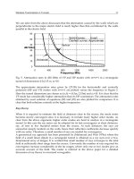
Fig. 5. Attenuation rates in dB/100m of VP and HP modes with m=n=1 in a rectangular
tunnel of dimensions 4.3x2.15 m.

r
=10.

The approximate attenuation rates given by (27-28) for the horizontally and vertically
polarized (HP and VP) modes with m=n=1 are plotted versus the frequency in Figure 5.
Here the tunnel dimensions are chosen as (w,h) = (4.3m, 2.15m) and 
r

=10. It is clear that the
VP mode has considerably higher attenuation than its HP counterpart. The attenuation rates
obtained by exact solution of equations (22) and (25) are also plotted for comparison. It is
clear that both solutions coincide at the higher frequencies.

Ray theory:

When it is required to estimate the field at distances close to the source, the mode series
becomes slowly convergent since it is necessary to include many higher order modes. As
clear from the above argument, higher order modes are hard to analyze in a rectangular
tunnel. In this case the ray series can be adopted for its fast convergence at short distances,
say, of tens to few hundred meters from the source. At such distances, the rays are
somewhat steeply incident on the walls, hence their reflection coefficients decrease quickly
with ray order. Therefore, a small number of rays are needed for convergence.
A geometrical ray approach has been presented by (Mahmoud and Wait 1974a) where the
field of a small linear dipole in a rectangular tunnel is obtained as a ray sum over a two-
dimensional array of images. It is verified that small number of rays converges to the total
field at sufficiently short range from the source. Conversely the number of rays required for
convergence increase considerably in the far ranges, where only one or two modes give an
accurate account of the field. The reader is referred to the above paper for a detailed
discussion of ray theory in oversized waveguides.
0
10
20
30
40
50
60
0 400 800 1200 1600 2000
dB/100m

Frequency MHz
Horizontal
Vertical
Solid Curves: Exact
Dashed curves: Approximate
MobileandWirelessCommunications:Physicallayerdevelopmentandimplementation12

5. Arched Tunnel

So far we have been studying tunnels with regular cross sections having either circular or
rectangular shape. These shapes are amenable to analytical analysis that lead to full
characterization of their main modes of propagation. However, most existing tunnels do not
have regular cross sections and their study may require exhaustive numerical methods
(Pingenot et al., 2006). In this section we consider cylindrical tunnels whose cross-section
comprise a circular arch with a flat base as depicted in Figure 6. This can be considered as a
circular tunnel whose shape is perturbed into a flat-based tunnel. So, we use the
perturbation theory to predict attenuation and phase velocity of the dominant modes from
those in a perfectly circular tunnel.

Fig. 6. An arched tunnel with radius a and flat base L.

5.1. Perturbation Analysis
We consider a cylindrical circular tunnel of radius ‘a’ and cross section S
0
surrounded by a
homogeneous earth of relative permittivity

r
. Let us denote the vector fields of a given
mode by
0 0 0
( , )exp( )E H z


 
where
0

is the longitudinal (along +z) propagation constant.
Similarly, let
( , )exp( )
E
H z


 
be the vector fields of the corresponding mode in the perturbed
tunnel of of area S (Figure 7). Note, however, that the mode is a backward mode; travelling

in the (-z) direction. Both circular and perturbed tunnels have the same wall constant
impedance Z and admittance Y. Now, we use Maxwell’s equations that must be satisfied by
both modal fields to get the reciprocity relation
0 0
.( ) 0E H E H    

  
. Integrating over the
infinitesimal volume between z and z+dz in the perturbed tunnel, we get, after some
manipulations,
L
x

y

Fig. 7. A circular tunnel and a perturbed circular tunnel with a flat base. The walls are
characterized by constant Z and Y.

0 0 1
1
0
0 0
ˆ
( ).
ˆ
( ).
n

C
z
S
E
xH ExH a dC
E
xH ExH a dS
 
 
 




  
   
(29)

where C
1
is the flat part of the cross- section contour,
ˆ
n
a
is a unit vector along the outward
normal to the wall (=-
ˆ
y
a
) and

ˆ
z
a is a unit axial vector. The integration in the denominator is
taken over the cross section of the perturbed tunnel. In order to evaluate the numerator of
(2), we use the constant wall impedance and admittance satisfied by the perturbed fields on
the flat surface:
and
x
s z x s z
E
Z H H Y E   . Z
s
and Y
s
are given in (1-2). Using these relations,
(29) reduces to:

/ 2
0 0 0 0
0
0
0 0
2
ˆ
( ).
L
x z z x s z z s z z
x
z
S

E H E H Y E E Z H H dx
E xH ExH a dS
 

   




 



   
(30)

The integration in the numerator is taken over the flat surface of the perturbed tunnel. So
far, the above result is rigorous, but cannot be used as such since the perturbed fields are not
known. As a first approximation we can equate these fields to the backward mode fields in
the un-perturbed (circular) tunnel. So we set:
0 0
,
z
z z z
H H E E

  in the numerator. In the
denominator, the fields involved are the transverse fields (to z). So we use the
approximations:
0 0

ˆ ˆ ˆ ˆ
x x x x
z z z z
E a E a and H a H a  

  
. Therefore (30) is approximated by:

/ 2
2 2
0 0 0 0 0 0
0
0
0 0
ˆ
( x ).
L
x z z x s z s z
x
z
S
E H E H Y E Z H dx
E H a dS
 



  



 


 
(31)

Thus, for a given mode in the circular tunnel, (31) can be used to get the propagation
constant of the perturbed mode in the corresponding perturbed tunnel. Of particular
S

C
1

C
2

S
0

Z,Y

WirelessTransmissioninTunnels 13

5. Arched Tunnel

So far we have been studying tunnels with regular cross sections having either circular or
rectangular shape. These shapes are amenable to analytical analysis that lead to full
characterization of their main modes of propagation. However, most existing tunnels do not

have regular cross sections and their study may require exhaustive numerical methods
(Pingenot et al., 2006). In this section we consider cylindrical tunnels whose cross-section
comprise a circular arch with a flat base as depicted in Figure 6. This can be considered as a
circular tunnel whose shape is perturbed into a flat-based tunnel. So, we use the
perturbation theory to predict attenuation and phase velocity of the dominant modes from
those in a perfectly circular tunnel.

Fig. 6. An arched tunnel with radius a and flat base L.

5.1. Perturbation Analysis
We consider a cylindrical circular tunnel of radius ‘a’ and cross section S
0
surrounded by a
homogeneous earth of relative permittivity

r
. Let us denote the vector fields of a given
mode by

0 0 0
( , )exp( )E H z


 
where
0

is the longitudinal (along +z) propagation constant.
Similarly, let
( , )exp( )
E
H z


 
be the vector fields of the corresponding mode in the perturbed
tunnel of of area S (Figure 7). Note, however, that the mode is a backward mode; travelling
in the (-z) direction. Both circular and perturbed tunnels have the same wall constant
impedance Z and admittance Y. Now, we use Maxwell’s equations that must be satisfied by
both modal fields to get the reciprocity relation
0 0
.( ) 0E H E H

   

  
. Integrating over the
infinitesimal volume between z and z+dz in the perturbed tunnel, we get, after some
manipulations,

L
x

y

Fig. 7. A circular tunnel and a perturbed circular tunnel with a flat base. The walls are
characterized by constant Z and Y.

0 0 1
1
0
0 0
ˆ
( ).
ˆ
( ).
n
C
z
S
E
xH ExH a dC
E
xH ExH a dS
 
 
 





  
   
(29)

where C
1
is the flat part of the cross- section contour,
ˆ
n
a
is a unit vector along the outward
normal to the wall (=-
ˆ
y
a
) and
ˆ
z
a is a unit axial vector. The integration in the denominator is
taken over the cross section of the perturbed tunnel. In order to evaluate the numerator of
(2), we use the constant wall impedance and admittance satisfied by the perturbed fields on
the flat surface:
and
x
s z x s z
E

Z H H Y E   . Z
s
and Y
s
are given in (1-2). Using these relations,
(29) reduces to:

/ 2
0 0 0 0
0
0
0 0
2
ˆ
( ).
L
x z z x s z z s z z
x
z
S
E H E H Y E E Z H H dx
E xH ExH a dS
 

   
 
 
 




   
(30)

The integration in the numerator is taken over the flat surface of the perturbed tunnel. So
far, the above result is rigorous, but cannot be used as such since the perturbed fields are not
known. As a first approximation we can equate these fields to the backward mode fields in
the un-perturbed (circular) tunnel. So we set:
0 0
,
z
z z z
H H E E   in the numerator. In the
denominator, the fields involved are the transverse fields (to z). So we use the
approximations:
0 0
ˆ ˆ ˆ ˆ
x x x x
z z z z
E a E a and H a H a  

  
. Therefore (30) is approximated by:

/ 2
2 2
0 0 0 0 0 0
0

0
0 0
ˆ
( x ).
L
x z z x s z s z
x
z
S
E H E H Y E Z H dx
E H a dS
 

 
  
 
 


 
(31)

Thus, for a given mode in the circular tunnel, (31) can be used to get the propagation
constant of the perturbed mode in the corresponding perturbed tunnel. Of particular
S

C
1

C

2

S
0

Z,Y

MobileandWirelessCommunications:Physicallayerdevelopmentandimplementation14
interest is the attenuation factor of the various modes. As a numerical example, we consider
an arched tunnel of radius a=2meters with a flat base of width L. The surrounding earth has
a relative permittivity

r
=6. For an applied frequency f =500MHz, the modal attenuation
factor, computed by (31), is plotted in Figure 8 for the perturbed TE
01
and HE
11
modes as a
function of the L/a. Note that L/a=0 corresponds to a full circle and L/a=2 corresponds to a
half circle. Generally the attenuation increases with L/a. The HE
11
mode has two versions
depending whether the polarization is horizontal (along x) or vertical (along y). Obviously
the two modes are degenerate in a perfectly circular tunnel (L=0). However as L/a increases,
this degeneracy breaks down in the perturbed tunnel. It is remarkable to see that the
attenuation of the horizontally polarized HE
11
mode becomes less than that of the vertically
polarized mode in the perturbed tunnel. This agrees with measurements made by Molina et

al. (2008).
It is interesting to study the effect of changing the frequency or the wall permittivity on the
mode attenuation in the perturbed flat based tunnel. Further numerical results (not shown)
indicate that the percentage increase of the attenuation relative to that in the circular tunnel
is fairly weak on f and

r
. Since the attenuation in an electrically large circular tunnel is
inversely proportional to f
2
, so will be the attenuation in the perturbed flat based tunnel.

Fig. 8. Attenuation of the perturbed TE

01
and HE
11
modes in a flat based tunnel versus L/a.
Note the difference between the attenuation of the VP and the HP versions of the HE
11

mode.

5.2. An equivalent rectangular tunnel
As seen in Figure 8, the attenuation of the perturbed HE
11
mode in the arched tunnel (with
flat base) depends on the mode polarization; namely the vertically polarized HE
11
mode is
more attenuated than the horizontally polarized mode. The same observation is true for the
HE
11
mode in a rectangular tunnel whose height ‘h’ is less than its width ‘w’. This raises the
question whether we can model the flat based tunnel of Figure 6 by a rectangular tunnel.
We will investigate this possibility in this section. To this end, let us start by comparing the
0
5
10
15
20
0 0,5 1 1,5 2
Mode Atten. dB/100m
L/a

TE10
HE11,
H-pol
HE11,
V-
p
ol
a=2m
f=500 MHz

r
=6
attenuation of the HE
nm
mode in tunnels with circular and a square cross sections. For the
circular tunnel we have from (15)

2
0 0
1,
2 3
0
/
|
2
s s
HEnm n m
Z Y
x

k a
 








(32)

Where
1,n m
x

is the mth zero of the Bessel function J
n-1
(x). This formula is based on the
condition:
0 1,n m
k a x


. For the rectangular tunnel with width ‘w’ and height ‘h’ the
attenuation of the HE
nm
mode (with vertical polarization) is given by (27) which is repeated
here

2 2
2
0 0
2 3 3
0
/
2
|
s s
HEnm
m Z n Y
k w h






 






(33)

This is valid for electrically large tunnel, or when
0
/ and /k m w n h



 . Specializing this
result for the HE
11
mode in a square tunnel (w=h and m=n=1) , we get:

2
11 0 0
2 3
0
2
| /
HE s s
Z Y
k w


 
 




(34)

Now compare the circular tunnel with the square tunnel for the HE
11
mode. From (32) and

(33), an equal attenuation occurs when

 
1/3
2 2
w 4 / 2.4048 1.897a a

 
(33)

which means that the area of the equivalent square tunnel is equal to 1.145 times the area of
the circular tunnel. This contrasts the work of (Dudley et.al, 2007) who adopted an equal
area of tunnels. It is important to note that this equivalence is valid only for the HE
11
mode
in both tunnels; for other modes the attenuation in the circular and the square tunnels are
generally not equal.
Now let us turn attention to the arched tunnel with flat base (Figure 6) for which we attempt
to find an equivalent rectangular tunnel. We base this equivalence on equal attenuation of
the HE
11
mode in both tunnels. Let us maintain the ratio of areas as obtained from the
square and circular tunnels; namely we fix the ratio of the equivalent rectangular area to the
arched tunnel area to 1.145. Meanwhile we choose the ratio h/w equal to the arched tunnel
height to its diameter. So, we write:

2
1.145[( ) ( / 2)cos ], and
/ (1 cos ) / 2

wh a La
h w
  

  
 
(34)

where
Arcsin( / 2 )L a


is equal to half the angle subtended by the flat base L at the center
of the circle.
WirelessTransmissioninTunnels 15
interest is the attenuation factor of the various modes. As a numerical example, we consider
an arched tunnel of radius a=2meters with a flat base of width L. The surrounding earth has
a relative permittivity

r
=6. For an applied frequency f =500MHz, the modal attenuation
factor, computed by (31), is plotted in Figure 8 for the perturbed TE
01
and HE
11
modes as a
function of the L/a. Note that L/a=0 corresponds to a full circle and L/a=2 corresponds to a
half circle. Generally the attenuation increases with L/a. The HE
11
mode has two versions

depending whether the polarization is horizontal (along x) or vertical (along y). Obviously
the two modes are degenerate in a perfectly circular tunnel (L=0). However as L/a increases,
this degeneracy breaks down in the perturbed tunnel. It is remarkable to see that the
attenuation of the horizontally polarized HE
11
mode becomes less than that of the vertically
polarized mode in the perturbed tunnel. This agrees with measurements made by Molina et
al. (2008).
It is interesting to study the effect of changing the frequency or the wall permittivity on the
mode attenuation in the perturbed flat based tunnel. Further numerical results (not shown)
indicate that the percentage increase of the attenuation relative to that in the circular tunnel
is fairly weak on f and

r
. Since the attenuation in an electrically large circular tunnel is
inversely proportional to f
2
, so will be the attenuation in the perturbed flat based tunnel.

Fig. 8. Attenuation of the perturbed TE
01
and HE
11
modes in a flat based tunnel versus L/a.
Note the difference between the attenuation of the VP and the HP versions of the HE
11

mode.

5.2. An equivalent rectangular tunnel
As seen in Figure 8, the attenuation of the perturbed HE
11
mode in the arched tunnel (with
flat base) depends on the mode polarization; namely the vertically polarized HE
11
mode is
more attenuated than the horizontally polarized mode. The same observation is true for the
HE
11
mode in a rectangular tunnel whose height ‘h’ is less than its width ‘w’. This raises the
question whether we can model the flat based tunnel of Figure 6 by a rectangular tunnel.
We will investigate this possibility in this section. To this end, let us start by comparing the
0

5
10
15
20
0 0,5 1 1,5 2
Mode Atten. dB/100m
L/a
TE10
HE11,
H-pol
HE11,
V-
p
ol
a=2m
f=500 MHz

r
=6
attenuation of the HE
nm
mode in tunnels with circular and a square cross sections. For the
circular tunnel we have from (15)

2
0 0
1,
2 3
0

/
|
2
s s
HEnm n m
Z Y
x
k a
 



 

 
(32)

Where
1,n m
x

is the mth zero of the Bessel function J
n-1
(x). This formula is based on the
condition:
0 1,n m
k a x


. For the rectangular tunnel with width ‘w’ and height ‘h’ the

attenuation of the HE
nm
mode (with vertical polarization) is given by (27) which is repeated
here

2 2
2
0 0
2 3 3
0
/
2
|
s s
HEnm
m Z n Y
k w h




 
 
 
 
 
(33)

This is valid for electrically large tunnel, or when
0

/ and /k m w n h


 . Specializing this
result for the HE
11
mode in a square tunnel (w=h and m=n=1) , we get:

2
11 0 0
2 3
0
2
| /
HE s s
Z Y
k w


 
 
 
 
(34)

Now compare the circular tunnel with the square tunnel for the HE
11
mode. From (32) and
(33), an equal attenuation occurs when

 
1/3
2 2
w 4 / 2.4048 1.897a a

 
(33)

which means that the area of the equivalent square tunnel is equal to 1.145 times the area of
the circular tunnel. This contrasts the work of (Dudley et.al, 2007) who adopted an equal
area of tunnels. It is important to note that this equivalence is valid only for the HE
11
mode
in both tunnels; for other modes the attenuation in the circular and the square tunnels are
generally not equal.
Now let us turn attention to the arched tunnel with flat base (Figure 6) for which we attempt
to find an equivalent rectangular tunnel. We base this equivalence on equal attenuation of
the HE
11
mode in both tunnels. Let us maintain the ratio of areas as obtained from the
square and circular tunnels; namely we fix the ratio of the equivalent rectangular area to the
arched tunnel area to 1.145. Meanwhile we choose the ratio h/w equal to the arched tunnel
height to its diameter. So, we write:

2
1.145[( ) ( / 2)cos ], and
/ (1 cos ) / 2
wh a La

h w
  

  
 
(34)

where
Arcsin( / 2 )L a


is equal to half the angle subtended by the flat base L at the center
of the circle.
MobileandWirelessCommunications:Physicallayerdevelopmentandimplementation16

Fig. 9. Attenuation of the HE

11
mode in the arched tunnel of Figure 6 using perturbation
analysis and rectangular equivalent tunnel

Equation (34) defines the rectangular tunnel that is equivalent to the perturbed circular
tunnel regarding the HE
11
mode. In order to check the validity of this equivalence, we
compare the estimated attenuation of the HE
11
mode in the perturbed circular tunnel as
obtained by perturbation analysis and by the equivalent rectangular tunnel in Figure 9.
There is a reasonably close agreement between both methods of estimation for values of L/a
between zero and ~1.82.

6. Curved Tunnel

Modal propagation in a curved rectangular tunnel has been considered by Mahmoud and
Wait (1974b) and more recently by Mahmoud (2005). The model used is shown in Figure 10
where the curved surfaces coincide with

=R-w/2 and

=R+w/2 in a cylindrical frame (

,z )
with z parallel to the side walls. The tunnel is curved in the horizontal plane with assumed
gentle curvature so that the mean radius of curvature R is >>w. The analysis is made in the
high frequency regime so that k
0

w >>1. The modes are nearly TE or TM to z with horizontal
or vertical polarization respectively. The modal equations for the lower order TE
z
and TM
z

modes are derived in terms of the Airy functions and solved numerically for the
propagation constant along the
- direction. Numerical results are given in (Mahmoud,
2005) and are reproduced here in figures 11 and 12 for the dominant mode with vertical and
horizontal polarization respectively. It is seen that wall curvature causes drastic increase of
the attenuation especially for the horizontally polarized mode.
This can be explained by noting that the horizontal electric field is perpendicular to the
curved walls, causing more attenuation to incur for this polarization.

Further study of the modal fields shows that these fields cling towards the outer curved
wall casing increased losses in the wall. Besides, the mode velocity slows down.

0
5
10
15
20
0 0,5 1 1,5 2
Mode Atten. dB/100m
L/a
HE11,
HE11,
V-pol

____
perturbation
analysis
Rect. Model
a=2m
f=500
MHz

Fig. 10. A curved rectangular tunnel

Fig. 11. Attenuation of TM
y11
( VP) mode in a curved tunnel

Fig. 12. Attenuation of TM
x11
(HP) mode in a curved tunnel
Radius R

w

h
z


0.1
1
10
100
200 600 1000 1400 1800
Frequency (MHz)
Attenuation in dB/100m
Straight Tunnel
R=20w
w
h
E
w=2h=4.26m
0.1
1
10
100
200 600 1000 1400 1800
Frequency (MHz)
Attenuation in dB/100m
Straight Tunnel
R=50 a
R=10 a
w=2h=4.26
E
w

h
WirelessTransmissioninTunnels 17

Fig. 9. Attenuation of the HE
11
mode in the arched tunnel of Figure 6 using perturbation
analysis and rectangular equivalent tunnel

Equation (34) defines the rectangular tunnel that is equivalent to the perturbed circular
tunnel regarding the HE
11
mode. In order to check the validity of this equivalence, we
compare the estimated attenuation of the HE
11
mode in the perturbed circular tunnel as
obtained by perturbation analysis and by the equivalent rectangular tunnel in Figure 9.

There is a reasonably close agreement between both methods of estimation for values of L/a
between zero and ~1.82.

6. Curved Tunnel

Modal propagation in a curved rectangular tunnel has been considered by Mahmoud and
Wait (1974b) and more recently by Mahmoud (2005). The model used is shown in Figure 10
where the curved surfaces coincide with

=R-w/2 and

=R+w/2 in a cylindrical frame (

,z )
with z parallel to the side walls. The tunnel is curved in the horizontal plane with assumed
gentle curvature so that the mean radius of curvature R is >>w. The analysis is made in the
high frequency regime so that k
0
w >>1. The modes are nearly TE or TM to z with horizontal
or vertical polarization respectively. The modal equations for the lower order TE
z
and TM
z

modes are derived in terms of the Airy functions and solved numerically for the
propagation constant along the
- direction. Numerical results are given in (Mahmoud,
2005) and are reproduced here in figures 11 and 12 for the dominant mode with vertical and
horizontal polarization respectively. It is seen that wall curvature causes drastic increase of
the attenuation especially for the horizontally polarized mode.

This can be explained by noting that the horizontal electric field is perpendicular to the
curved walls, causing more attenuation to incur for this polarization.

Further study of the modal fields shows that these fields cling towards the outer curved
wall casing increased losses in the wall. Besides, the mode velocity slows down.

0
5
10
15
20
0 0,5 1 1,5 2
Mode Atten. dB/100m
L/a
HE11,
HE11,
V-pol
____
perturbation
analysis
Rect. Model
a=2m
f=500
MHz

Fig. 10. A curved rectangular tunnel

Fig. 11. Attenuation of TM
y11
( VP) mode in a curved tunnel

Fig. 12. Attenuation of TM
x11
(HP) mode in a curved tunnel
Radius R

w
h
z

0.1
1
10
100
200 600 1000 1400 1800
Frequency (MHz)
Attenuation in dB/100m
Straight Tunnel
R=20w

w
h
E
w=2h=4.26m
0.1
1
10
100
200 600 1000 1400 1800
Frequency (MHz)
Attenuation in dB/100m
Straight Tunnel
R=50 a
R=10 a
w=2h=4.26
E
w
h
MobileandWirelessCommunications:Physicallayerdevelopmentandimplementation18
7. Experimental work

Measurements of attenuation of the dominant mode in a straight rectangular mine tunnel
were given by Goddard (1973). The tunnel cross section was 14x7 feet (or 4.26x2.13m) and
the external medium had

r
=10 and the attenuation was measured at 200, 450 and 1000
MHz. Emslie et al [25] compared these measurements with their theoretical values for the
dominant horizontally polarized mode. Good agreement was observed at the first two
frequencies, but the experimental values were considerably higher than the theoretical

attenuation at the 1000 MHz. Similar trend has also been reported more recently by Lienard
and Degauque (2000). The difference between the measured and theoretical attenuation at
the 1000 MHz was attributed by Emslie et al.(1975) to slight tilt of the tunnel walls. Namely,
by using a rather simple theory, it was shown that the increase of attenuation of the
dominant mode due to wall tilt is proportional to the frequency and the square of the tilt
angle. As a result, it was deduced that the high frequency attenuation of the dominant mode
in a rectangular tunnel is governed mainly by the wall tilt.
Goddard (1973) has also measured the signal level around a corner and inside a crossed
tunnel. The attenuation rate was very high for a short distance after which the attenuation
approaches that of the dominant horizontally polarized mode. Emslie et al. (1975) have
explained such behavior as follows. They argue that the crossed tunnel is excited by the
higher order modes (or diffused waves in their terms) in the main tunnel. The modes
excited in the crossed tunnel are mostly higher order modes with a small component of the
dominant mode. These high order modes exhibit very high attenuation for a short distance
after which the dominant mode becomes the sole propagating mode. So the signal level
starts with a large attenuation rate which gradually decreases towards the attenuation rate
of the dominant mode. The theory presented accordingly shows good agreement with
measurements. More recently, Lee and Bertoni (2003) evaluated the modal coupling for
tunnels or streets with L, T or cross junctions using hybrid ray-mode conversion. They argue
that coupling occurs by rays diffracted at the corners into the side tunnels. It is found that
the coupling loss is greatest at L-bends and least for cross junctions.
Chiba et.al (1975) have provided field measurements in one of the National Japanese
Railway tunnels located in Tohoku. The tunnel cross section is an arch with a flat base as
that depicted in Figure 6. The radius a=4.8 m, L=8.8m (L/a=1.83), the wall

r
=5.5 and = 0.03
S/m. Field measurements were taken down the tunnel for different frequencies and
polarizations. The attenuation of the dominant HE
11

mode was then measured for both
horizontal and vertical polarization at the frequencies 150, 470, 900, 1700, and 4000 MHz. We
plot the predicted attenuation of the horizontally polarized HE
11
mode in this same tunnel
using both the perturbation analysis and the rectangular tunnel model in Figure 13. On top
of these curves, the measured attenuation is shown as discrete dots at the above selected
frequencies. The predicted attenuation shows the expected inverse frequency squared
dependence. The measured attenuation follows the predicted attenuation except at the
highest two frequencies (1700 and 4000 MHz) whence it is higher than predicted. This can
be explained on account of wall roughness or micro-bending of the tunnel walls that affect
the higher frequencies in particular.

Fig. 13. Attenuation of the HE
11
mode in the Japanese National Ralway tunnel by the
perturbation analysis and the rectangular tunnel model versus measured values (as
reported in (Chiba et al., 1973).

Measurements of the electric field down the Massif Central road tunnel south Central
France have been taken by the research group in Lille University and the results are
reported by Dudley et.al. (2007). The Massif Central tunnel has a flat based circular arch
shape as in Figure 6 with radius a= 4.3 m and L=7.8 m; that is L/a= 1.81. The relative
permittivity of the wall

r
=5 and the conductivity = 0.01 S/m. The transmit and receive
antennas were vertically polarized and the field measured down the tunnel at the
frequencies 450 and 900 MHz are given in Figure 14. For the lower frequency, the field
shows fast oscillatory behavior in the near zone, but at far distances from the source (greater
than ~1800m), the field exhibits almost a constant rate of attenuation, which is that of the
dominant HE
11
(like) mode. We estimate the attenuation of this mode as 27.2 dB/km. At the
900 MHz frequency, there are two interfering modes that are observed in the range of 1500-
2500m. One of these two modes must be the dominant HE
11
mode. Some analysis is needed
in this range that lead to an estimation of the attenuation of the HE
11

mode, which we find
as 6.8 dB/km.
0.1
1
10
100
1000
0.1 1 10
Frequency (GHz)
Attenuation dB/km
Solid Line: Perturbation analysis
Dashed Line :Rectangular Model
Dots: Experimental (Chiba et al.,
1973)

r=5.5

=
0.03 S/m
WirelessTransmissioninTunnels 19
7. Experimental work

Measurements of attenuation of the dominant mode in a straight rectangular mine tunnel
were given by Goddard (1973). The tunnel cross section was 14x7 feet (or 4.26x2.13m) and
the external medium had

r
=10 and the attenuation was measured at 200, 450 and 1000
MHz. Emslie et al [25] compared these measurements with their theoretical values for the
dominant horizontally polarized mode. Good agreement was observed at the first two

frequencies, but the experimental values were considerably higher than the theoretical
attenuation at the 1000 MHz. Similar trend has also been reported more recently by Lienard
and Degauque (2000). The difference between the measured and theoretical attenuation at
the 1000 MHz was attributed by Emslie et al.(1975) to slight tilt of the tunnel walls. Namely,
by using a rather simple theory, it was shown that the increase of attenuation of the
dominant mode due to wall tilt is proportional to the frequency and the square of the tilt
angle. As a result, it was deduced that the high frequency attenuation of the dominant mode
in a rectangular tunnel is governed mainly by the wall tilt.
Goddard (1973) has also measured the signal level around a corner and inside a crossed
tunnel. The attenuation rate was very high for a short distance after which the attenuation
approaches that of the dominant horizontally polarized mode. Emslie et al. (1975) have
explained such behavior as follows. They argue that the crossed tunnel is excited by the
higher order modes (or diffused waves in their terms) in the main tunnel. The modes
excited in the crossed tunnel are mostly higher order modes with a small component of the
dominant mode. These high order modes exhibit very high attenuation for a short distance
after which the dominant mode becomes the sole propagating mode. So the signal level
starts with a large attenuation rate which gradually decreases towards the attenuation rate
of the dominant mode. The theory presented accordingly shows good agreement with
measurements. More recently, Lee and Bertoni (2003) evaluated the modal coupling for
tunnels or streets with L, T or cross junctions using hybrid ray-mode conversion. They argue
that coupling occurs by rays diffracted at the corners into the side tunnels. It is found that
the coupling loss is greatest at L-bends and least for cross junctions.
Chiba et.al (1975) have provided field measurements in one of the National Japanese
Railway tunnels located in Tohoku. The tunnel cross section is an arch with a flat base as
that depicted in Figure 6. The radius a=4.8 m, L=8.8m (L/a=1.83), the wall

r
=5.5 and = 0.03
S/m. Field measurements were taken down the tunnel for different frequencies and
polarizations. The attenuation of the dominant HE

11
mode was then measured for both
horizontal and vertical polarization at the frequencies 150, 470, 900, 1700, and 4000 MHz. We
plot the predicted attenuation of the horizontally polarized HE
11
mode in this same tunnel
using both the perturbation analysis and the rectangular tunnel model in Figure 13. On top
of these curves, the measured attenuation is shown as discrete dots at the above selected
frequencies. The predicted attenuation shows the expected inverse frequency squared
dependence. The measured attenuation follows the predicted attenuation except at the
highest two frequencies (1700 and 4000 MHz) whence it is higher than predicted. This can
be explained on account of wall roughness or micro-bending of the tunnel walls that affect
the higher frequencies in particular.

11
mode, which we find
as 6.8 dB/km.
0.1
1
10
100
1000
0.1 1 10
Frequency (GHz)
Attenuation dB/km
Solid Line: Perturbation analysis
Dashed Line :Rectangular Model
Dots: Experimental (Chiba et al.,
1973)

r=5.5

=
0.03 S/m
MobileandWirelessCommunications:Physicallayerdevelopmentandimplementation20
5 0 0 1 0 0 0 1 5 0 0 2 0 0 0 2 5 0 0
- 1 1 0
- 1 0 0
- 9 0
- 8 0
- 7 0
- 6 0
- 5 0
- 4 0

- 3 0
- 2 0
- 1 0
P u i s s a n c e r e ç u e ( d B m )
d i s t a n c e ( m )
9 0 0 M H z
4 5 0 M H z

Fig. 14. Measured field down the Massif Central Tunnel in South France (Dudley et al., 2007)
at 450 and 900 MHz.

A comparison between these measured attenuation rates and those predicted by the
perturbation analysis or the equivalent rectangular tunnel (given in section 5) is made in
Table 2. Good agreement is seen between predicted and measured attenuation although the
measured values are slightly higher. This can be attributed to wall roughness and
microbending.

Perturbation
Analysis (dB/km)
Equivalent
Rectangular model
Measured
Attenuation
f =450 MHz 22.0 24.1 27.2
f =900 MHz 5.52 6.03 6.8
Table 2. Measured versus predicted attenuation rates of the HE
11
mode in the Massif Central

Road Tunnel, South France.

8. Concluding discussion

We have presented an account of wireless transmission of electromagnetic waves in mine and
road tunnels. Such tunnels act as oversized waveguides to UHF and the upper VHF waves.
The theory of mode propagation in straight tunnels of circular, rectangular and arched cross
sections has been covered and it is demonstrated that the dominant modes attenuate with
rates that decrease with the applied frequency squared. We have also studied the increase of
mode attenuation caused by tunnel curvature. Comparison of the theory with existing
experimental measurements in real tunnels show good agreement except at the higher
frequencies at which wall roughness, and microbending can increase signal loss over that
predicted by the theory. While the higher order modes are highly attenuated and therefore
contribute to signal loss, they can be beneficial in allowing the use of Multiple Input - Multiple
Output (MIMO) technique to increase the channel capacity of tunnels. A detailed account of
this important topic is found in (Lienard et al, 2003) and (Molina et al., 2008).

9. References

Andersen, J.B.; Berntsen, S. & Dalsgaard, P. (1975). Propagation in rectangular waveguides
with arbitrary internal and external media, IEEE Transaction on Microwave Theory
and Technique, MTT-23, No. 7, pp. 555-560.
Chiba, J.; Sato, J.R.; Inaba, T; Kuwamoto, Y.; Banno, O. & Sato, R. “ Radio communication in
tunnels”, IEEE Transaction on Microwave Theory and Technique, MTT-26, No. 6,
June 1978.
Dudley, D.G. (2004). Wireless Propagation in Circular Tunnels, IEEE Transaction on Antennas
and Propagation, Vol. 53, n0.1, pp. 435-441.
Dudley, D.G. & Mahmoud, S.F. (2006). Linear source in a circular tunnel, IEEE Transaction on
Antennas and Propagation, Vol. 54, n0.7, pp. 2034-2048.
Dudley, D.G., Martine Lienard, Samir F. Mahmoud and Pierre Degauque, (2007) “Wireless

Propagation in Tunnels”, IEEE Antenna and Propagation magazine, Vol. 49, no. 2, pp.
11-26, April 2007.
Emslie, A.G.; Lagace, R.L. & Strong, P.F. (1973). Theory of the propagation of UHF radio
waves in coal mine tunnels, Proc. Through the Earth Electromagnetics Workshop,
Colorado School of mines, Golden, Colorado, Aug. 15-17.
Emslie, A.G.; Lagace R.L. & Strong, P.F. (1975). Theory of the propagation of UHF radio
waves in coal mine tunnels, IEEE Transaction on Antenn. Propagat., Vol. AP-23, No.
2, pp. 192-205.
Glaser, J.I. (1967). Low loss waves in hollow dielectric tubes, Ph.D. Thesis, M.I.T.
Glaser, J.I. (1969). Attenuation and guidance of modes in hollow dielectric waveguides, IEEE
Trans. Microwave Theory and Tech, Vol. MTT-17, pp.173-174.
Goddard, A.E. (1973). Radio propagation measurements in coal mines at UHF and VHF,
Proc. Through the Earth Electromagnetics Workshop, Colorado School of mines,
Golden, Colorado, Aug. 15-17.
Lee, J. & Bertoni, H.L. (2003). Coupling at cross, T and L junction in tunnels and urban street
canyons, IEEE Transaction on Antenn. Propagat., Vol. AP-51, No. 5, pp. 192-205,
pp.926-935.
Lienard, M. & Degauque, P. (2000). Natural wave propagation in mine environment, IEEE
Transaction on Antennas & propagate, Vol-AP-48, No.9, pp.1326-1339.
Lienard, M.; Degauque, P.; Baudet, J. & Degardin, D. (2003). Investigation on MIMO
Channels in Subway Tunnels, IEEE Journal on Selected Areas in Communication,
Vol. 21, No. 3, pp.332-339.
Mahmoud, S.F. & Wait, J.R. (1974a). Geometrical optical approach for electromagnetic wave
propagation in rectangular mine tunnels, Radio Science , Vol. 9, no. 12, pp. 1147-
1158.
WirelessTransmissioninTunnels 21
5 0 0 1 0 0 0 1 5 0 0 2 0 0 0 2 5 0 0
- 1 1 0
- 1 0 0
- 9 0

- 8 0
- 7 0
- 6 0
- 5 0
- 4 0
- 3 0
- 2 0
- 1 0
P u i s s a n c e r e ç u e ( d B m )
d i s t a n c e ( m )
9 0 0 M H z
4 5 0 M H z

Fig. 14. Measured field down the Massif Central Tunnel in South France (Dudley et al., 2007)
at 450 and 900 MHz.

A comparison between these measured attenuation rates and those predicted by the
perturbation analysis or the equivalent rectangular tunnel (given in section 5) is made in
Table 2. Good agreement is seen between predicted and measured attenuation although the
measured values are slightly higher. This can be attributed to wall roughness and
microbending.

Perturbation
Analysis (dB/km)
Equivalent
Rectangular model
Measured
Attenuation

f =450 MHz 22.0 24.1 27.2
f =900 MHz 5.52 6.03 6.8
Table 2. Measured versus predicted attenuation rates of the HE
11
mode in the Massif Central
Road Tunnel, South France.

8. Concluding discussion

We have presented an account of wireless transmission of electromagnetic waves in mine and
road tunnels. Such tunnels act as oversized waveguides to UHF and the upper VHF waves.
The theory of mode propagation in straight tunnels of circular, rectangular and arched cross
sections has been covered and it is demonstrated that the dominant modes attenuate with
rates that decrease with the applied frequency squared. We have also studied the increase of
mode attenuation caused by tunnel curvature. Comparison of the theory with existing
experimental measurements in real tunnels show good agreement except at the higher
frequencies at which wall roughness, and microbending can increase signal loss over that
predicted by the theory. While the higher order modes are highly attenuated and therefore
contribute to signal loss, they can be beneficial in allowing the use of Multiple Input - Multiple
Output (MIMO) technique to increase the channel capacity of tunnels. A detailed account of
this important topic is found in (Lienard et al, 2003) and (Molina et al., 2008).

9. References

Andersen, J.B.; Berntsen, S. & Dalsgaard, P. (1975). Propagation in rectangular waveguides
with arbitrary internal and external media, IEEE Transaction on Microwave Theory
and Technique, MTT-23, No. 7, pp. 555-560.
Chiba, J.; Sato, J.R.; Inaba, T; Kuwamoto, Y.; Banno, O. & Sato, R. “ Radio communication in
tunnels”, IEEE Transaction on Microwave Theory and Technique, MTT-26, No. 6,
June 1978.

Dudley, D.G. (2004). Wireless Propagation in Circular Tunnels, IEEE Transaction on Antennas
and Propagation, Vol. 53, n0.1, pp. 435-441.
Dudley, D.G. & Mahmoud, S.F. (2006). Linear source in a circular tunnel, IEEE Transaction on
Antennas and Propagation, Vol. 54, n0.7, pp. 2034-2048.
Dudley, D.G., Martine Lienard, Samir F. Mahmoud and Pierre Degauque, (2007) “Wireless
Propagation in Tunnels”, IEEE Antenna and Propagation magazine, Vol. 49, no. 2, pp.
11-26, April 2007.
Emslie, A.G.; Lagace, R.L. & Strong, P.F. (1973). Theory of the propagation of UHF radio
waves in coal mine tunnels, Proc. Through the Earth Electromagnetics Workshop,
Colorado School of mines, Golden, Colorado, Aug. 15-17.
Emslie, A.G.; Lagace R.L. & Strong, P.F. (1975). Theory of the propagation of UHF radio
waves in coal mine tunnels, IEEE Transaction on Antenn. Propagat., Vol. AP-23, No.
2, pp. 192-205.
Glaser, J.I. (1967). Low loss waves in hollow dielectric tubes, Ph.D. Thesis, M.I.T.
Glaser, J.I. (1969). Attenuation and guidance of modes in hollow dielectric waveguides, IEEE
Trans. Microwave Theory and Tech, Vol. MTT-17, pp.173-174.
Goddard, A.E. (1973). Radio propagation measurements in coal mines at UHF and VHF,
Proc. Through the Earth Electromagnetics Workshop, Colorado School of mines,
Golden, Colorado, Aug. 15-17.
Lee, J. & Bertoni, H.L. (2003). Coupling at cross, T and L junction in tunnels and urban street
canyons, IEEE Transaction on Antenn. Propagat., Vol. AP-51, No. 5, pp. 192-205,
pp.926-935.
Lienard, M. & Degauque, P. (2000). Natural wave propagation in mine environment, IEEE
Transaction on Antennas & propagate, Vol-AP-48, No.9, pp.1326-1339.
Lienard, M.; Degauque, P.; Baudet, J. & Degardin, D. (2003). Investigation on MIMO
Channels in Subway Tunnels, IEEE Journal on Selected Areas in Communication,
Vol. 21, No. 3, pp.332-339.
Mahmoud, S.F. & Wait, J.R. (1974a). Geometrical optical approach for electromagnetic wave
propagation in rectangular mine tunnels, Radio Science , Vol. 9, no. 12, pp. 1147-
1158.

MobileandWirelessCommunications:Physicallayerdevelopmentandimplementation22
Mahmoud, S.F. & Wait, J.R. (1974a). Guided electromagnetic waves in a curved rectangular
mine tunnel, Radio Science, May 1974, pp. 567-572.
Mahmoud, S.F. (1991) Electromagnetic Waveguides; theory and applications, IEE electromagnetic
waves series 32, Peter peregrinus Ltd. on behalf of IEE.
Mahmoud, S.F. (2005). Modal propagation of high frequency e.m. waves in straight and
curved tunnels within the earth, Journal of electromagnetic wave applications
(JEMWA), Vol. 19, No. 12, pp. 1611-1627.
Marcatili, E.A.J. & Schmeltzer, R.A. (1964). Hollow metallic and dielectric waveguides for
long distsnce optical transmission and lasers, The Bell System Technical Journal, Vol.
43, pp. 1783-1809, July 1964.
Molina-Garcia-Padro, J.M.; Lienard, M. , Nasr, A. & Degauque, P. (2008). On the possibility
of interpreting field variations and polarization in arched tunnels using a model of
propagation in rectangular or circular tunnels, IEEE Transaction on Antenn.
Propagat., Vol. AP-56, No. 4, pp. 1206-1211.
Molina-Garcia-Pardo, J. M.; Liénard, M.; Degauque, P.; Dudley, D.G. & and Juan-Llacer,
M.(2008). MIMO Channel Characteristics in Rectangular Tunnels from Modal
Theory, IEEE Transactions on Vehicular Technology, Vol 57, No. 3, pp.1974-1979.
Pingenot, J.; Rieben, R.N.; White, D.A.; & Dudley, D.G. (2006). Full wave analysis of RF
signal attenuation in a lossy rough surface cave using high order Time Domain
vector Finite Element method, Journal of Electromagnetic Wave Applications, Vol.20,
no. 12, pp. 1695-1705.
Stratton, J.A. (1941). Electromagnetic Theory, McGraw Hill, New York.
Wait, J.R (1967). A fundamental difficulty in the analysis of cylindrical waveguides with
impedance walls, Electronic Letters, Vol. 3, No. 2, pp. 87-88.
Wait, J.R. (1980). Propagation in rectangular tunnel with imperfectly conducting walls,
Electronic Letters, Vol. 16, No. 13, pp. 521-522.

10. Appendix

The transverse fields of a hybrid mode in a circular tunnel are obtained from the axial fields
by (Mahmoud, 1991, p. 7):

0
2 2
0
2 2
ˆ
x
ˆ
z x
t t z t z
t t z t z
j
j
E E E z
k k
j
j
H H E
k k
 
 





   


   


(A1)
Where
t

is the transverse differential operator:
ˆ ˆ
( / ) ( / )
t
    
       .
Using the axial fields in (5) we get the explicit expressions:

0
0
0
0
( )
( / ) ( ) sin
( )
( / ) ( ) cos
n
j z
n
n
j z
n

nJ k
k
E k J k n e
k k
nJ k
k
E k J k n e
k k


 
 


 
 

  


  



 

  
 
 
 

 

  
 
 
 
(A2)

And

0
0 0
0
0 0
( )
( / ) ( ) cos
( )
( / ) ( ) sin
n
j z
n
n
j z
n
nJ k
k
H k J k n e
k k
nJ k
k

H k J k n e
k k


 
 


 
 

   


   



 

   
 
 
 
 

  
 
 
 

(A3)

It is useful to express the transverse field in terms of Cartesian coordinates (x,y). Using the
Bessel function identities:

1 1
1 1
( )/ ( ( ) ( ))/ 2
( ) ( ( ) ( )) / 2
n n n
n n n
nJ u u J u J u
J u J u J u
 
 
 

 
(A4)

we get:

0 1 0 1
0
0 1 0 1
0
2
[ / ] ( )sin( 1) [ / ] ( )sin( 1)
2

[ / ] ( ) cos( 1) [ / ] ( ) cos( 1)
x n n
y n n
k
E k J k n k J k n
k
k
E k J k n k J k n
k

 

 

    

    
 
 
        
       
(A5)

In the special case n=1, (A5) reduces to:

0 2
0
0 0 0 2
0
2

[ / ] ( )sin 2
2
[ / ] ( ) [ / ] ( ) cos2
x
y
k
E k J k
k
k
E k J k k J k
k



 
  

   
   
     
(A6)

This shows that for the HE
11
mode (~ +1), the field is almost y-polarized.
The corresponding magnetic field is

0 2
0
0 0 0 2

0
2
[ / 1] ( )sin 2
2
[ / 1] ( ) [ / 1] ( )cos 2
y
x
k
H k J k
k
k
H k J k k J k
k



 
  

   
  
      
(A7)

Equations (A6-A7) give the transverse fields of the HE
1m
modes.
WirelessTransmissioninTunnels 23
Mahmoud, S.F. & Wait, J.R. (1974a). Guided electromagnetic waves in a curved rectangular
mine tunnel, Radio Science, May 1974, pp. 567-572.

Mahmoud, S.F. (1991) Electromagnetic Waveguides; theory and applications, IEE electromagnetic
waves series 32, Peter peregrinus Ltd. on behalf of IEE.
Mahmoud, S.F. (2005). Modal propagation of high frequency e.m. waves in straight and
curved tunnels within the earth, Journal of electromagnetic wave applications
(JEMWA), Vol. 19, No. 12, pp. 1611-1627.
Marcatili, E.A.J. & Schmeltzer, R.A. (1964). Hollow metallic and dielectric waveguides for
long distsnce optical transmission and lasers, The Bell System Technical Journal, Vol.
43, pp. 1783-1809, July 1964.
Molina-Garcia-Padro, J.M.; Lienard, M. , Nasr, A. & Degauque, P. (2008). On the possibility
of interpreting field variations and polarization in arched tunnels using a model of
propagation in rectangular or circular tunnels, IEEE Transaction on Antenn.
Propagat., Vol. AP-56, No. 4, pp. 1206-1211.
Molina-Garcia-Pardo, J. M.; Liénard, M.; Degauque, P.; Dudley, D.G. & and Juan-Llacer,
M.(2008). MIMO Channel Characteristics in Rectangular Tunnels from Modal
Theory, IEEE Transactions on Vehicular Technology, Vol 57, No. 3, pp.1974-1979.
Pingenot, J.; Rieben, R.N.; White, D.A.; & Dudley, D.G. (2006). Full wave analysis of RF
signal attenuation in a lossy rough surface cave using high order Time Domain
vector Finite Element method, Journal of Electromagnetic Wave Applications, Vol.20,
no. 12, pp. 1695-1705.
Stratton, J.A. (1941). Electromagnetic Theory, McGraw Hill, New York.
Wait, J.R (1967). A fundamental difficulty in the analysis of cylindrical waveguides with
impedance walls, Electronic Letters, Vol. 3, No. 2, pp. 87-88.
Wait, J.R. (1980). Propagation in rectangular tunnel with imperfectly conducting walls,
Electronic Letters, Vol. 16, No. 13, pp. 521-522.

10. Appendix

The transverse fields of a hybrid mode in a circular tunnel are obtained from the axial fields
by (Mahmoud, 1991, p. 7):

0
2 2
0
2 2
ˆ
x
ˆ
z x
t t z t z
t t z t z
j
j
E E E z
k k
j
j
H H E
k k
 
 





   

   



(A1)
Where
t

is the transverse differential operator:
ˆ ˆ
( / ) ( / )
t

   
       .
Using the axial fields in (5) we get the explicit expressions:

0
0
0
0
( )
( / ) ( ) sin
( )
( / ) ( ) cos
n
j z
n
n
j z
n
nJ k
k

E k J k n e
k k
nJ k
k
E k J k n e
k k


 
 


 
 

  


  



 

  
 
 
 
 


  
 
 
 
(A2)

And

0
0 0
0
0 0
( )
( / ) ( ) cos
( )
( / ) ( ) sin
n
j z
n
n
j z
n
nJ k
k
H k J k n e
k k
nJ k
k
H k J k n e
k k



 
 


 
 

   


   



 

   
 
 
 
 

  
 
 
 
(A3)

It is useful to express the transverse field in terms of Cartesian coordinates (x,y). Using the
Bessel function identities:

1 1
1 1
( )/ ( ( ) ( ))/ 2
( ) ( ( ) ( )) / 2
n n n
n n n
nJ u u J u J u
J u J u J u
 
 
 

 
(A4)

we get:

0 1 0 1
0
0 1 0 1
0
2
[ / ] ( )sin( 1) [ / ] ( )sin( 1)
2
[ / ] ( ) cos( 1) [ / ] ( ) cos( 1)
x n n

y n n
k
E k J k n k J k n
k
k
E k J k n k J k n
k

 

 

    

    
 
 
        
       
(A5)

In the special case n=1, (A5) reduces to:

0 2
0
0 0 0 2
0
2
[ / ] ( )sin 2
2

[ / ] ( ) [ / ] ( ) cos2
x
y
k
E k J k
k
k
E k J k k J k
k



 
  

   
   
     
(A6)

This shows that for the HE
11
mode (~ +1), the field is almost y-polarized.
The corresponding magnetic field is

0 2
0
0 0 0 2
0
2

[ / 1] ( )sin 2
2
[ / 1] ( ) [ / 1] ( )cos 2
y
x
k
H k J k
k
k
H k J k k J k
k



 
  

   
  
      
(A7)

Equations (A6-A7) give the transverse fields of the HE
1m
modes.
MobileandWirelessCommunications:Physicallayerdevelopmentandimplementation24
WirelessCommunicationsandMultitaperAnalysis:
ApplicationstoChannelModellingandEstimation 25
Wireless Communications and Multitaper Analysis: Applications to
ChannelModellingandEstimation

SaharJavaherHaghighi,SergueiPrimak,ValeriKontorovichandErvinSejdić
0
Wireless Communications and Multitaper Analysis:
Applications to Channel Modelling and Estimation
Sahar Javaher Haghighi and Serguei Primak
Department of Electrical and Computer Engineering,
The University of Western Ontario
London, Ontario, Canada
Valeri Kontorovich
CINVESTAV
Mexico
Ervin Sejdi
´
c
Bloorview Research Institute
Institute of Biomaterials and Biomedical Engineering
University of Toronto
Toronto, Ontario, Canada
1. Introduction
The goal of this Chapter is to review the applications of the Thomson Multitaper analysis
(Percival and Walden; 1993b), (Thomson; 1982) for problems encountered in communications
(Thomson; 1998; Stoica and Sundin; 1999). In particular we will focus on issues related to
channel modelling, estimation and prediction.
Sum of Sinusoids (SoS) or Sum of Cisoids (SoC) simulators (Patzold; 2002; SCM Editors; 2006)
are popular ways of building channel simulators both in SISO and MIMO case. However,
this approach is not a very good option when features of communications systems such as
prediction and estimation are to be simulated. Indeed, representation of signals as a sum of
coherent components with large prediction horizon (Papoulis; 1991) leads to overly optimistic
results. In this Chapter we develop an approach which allows one to avoid this difﬁculty.
The proposed simulator combines a representation of the scattering environment advocated

in (SCM Editors; 2006; Almers et al.; 2006; Molisch et al.; 2006; Asplund et al.; 2006; Molish;
2004) and the approach for a single cluster environment used in (Fechtel; 1993; Alcocer et al.;
2005; Kontorovich et al.; 2008) with some important modiﬁcations (Yip and Ng; 1997; Xiao
et al.; 2005).
The problem of estimation and interpolation of a moderately fast fading Rayleigh/Rice chan-
nel is important in modern communications. The Wiener ﬁlter provides the optimum solution
when the channel characteristics are known (van Trees; 2001). However, in real-life applica-
tions basis expansions such as Fourier bases and discrete prolate spheroidal sequences (DPSS)
have been adopted for such problems (Zemen and Mecklenbr
¨
auker; 2005; Alcocer-Ochoa
et al.; 2006). If the bases and the channel under investigation occupy the same band, accurate
2
MobileandWirelessCommunications:Physicallayerdevelopmentandimplementation26
and sparse representations of channels are usually obtained (Zemen and Mecklenbr
¨
auker;
2005). However, a larger number of bases is required to approximate the channel with the
same accuracy when the bandwidth of the basis function is mismatched and larger than that
of the signal. A bank of bases with different bandwidths can be used to resolve this particu-
lar problem (Zemen et al.; 2005). However, such a representation again ignores the fact that
in some cases the band occupied by the channel is not necessarily centered around DC, but
rather at some frequency different from zero. Hence, a larger number of bases is again needed
for accurate and sparse representation. A need clearly exists for some type of overcomplete,
redundant bases which accounts for a variety of scenarios. A recently proposed overcomplete
set of bases called Modulated Discrete Prolate Spheroidal Sequences (MDPSS) (Sejdi
´
c et al.;
2008) resolves the aforementioned issues. The bases within the frame are obtained by modu-
lation and variation of the bandwidth of DPSSs in such a way as to reﬂect various scattering

scenarios.
2. Theoretical Background
2.1 Discrete Prolate Spheroidal Sequences
The technique used here was introduced ﬁrst in (Thomson; 1982) and further discussed in
(Percival and Walden; 1993b). We adopt notations used in the original paper (Thomson; 1982).
Let x
(n) be a ﬁnite duration segment of a stationary process, n = 0, ··· , N −1. It can be repre-
sented as
x
(n) =

1/2
−1/2
exp
(
j2π f [n −(N −1)/2]
)
dZ( f ) (1)
according to the Cramer theorem (Papoulis; 1991). It is emphasized in (Thomson; 1982) that
goal of the spectral analysis is to estimate moments of Z
( f ), in particular its ﬁrst and sec-
ond moments from a ﬁnite sample x
(n). However, spectral analysis is often reduced only to
considering the second centered moment
S
( f )d f = E

|dZ(f )|
2


(2)
well known as the spectrum (power spectral density). In the case of continuous spectrum the
ﬁrst moment of dZ
( f ) is zero and it is usually not considered. However, in the case of a line
or mixed spectrum one obtains
E
{
dZ( f )
}
=
∑
k
µ
k
δ( f − f
k
)d f (3)
where µ
k
is the amplitude of the harmonic with frequency f
k
.
The Discrete prolate spheroidal sequences (DPSS) are deﬁned as solutions to the Toeplitz ma-
trix eigenvalue problem (Thomson; 1982; Slepian; 1978)
λ
k
(N,W)u
k
(N,W;n) =
N−1

∑
m=0
sin
(
2W(n −m)
)
π(n −m)
u
k
(N,W;m) (4)
Their discrete Fourier transform (DFT) is known as Discrete Prolate Spheroidal Wave Func-
tions (DPSWF) (Slepian; 1978)
U
k
(N,W; f ) =
N−1
∑
n=0
u
k
(N,W;n)exp(−j 2πn f ) (5)
In particular, if f = 0, equation (5) can be rewritten as
U
k
(N,W;0) = U
k
(0) =
N−1
∑
n=0

u
k
(N,W;n) (6)
The DPSS are doubly orthogonal, that is, they are orthogonal on the inﬁnite set
{−∞, ,∞}
and orthonormal on the ﬁnite set {0,1, , N − 1}, that is,
∞
∑
−∞
v
i
(n,N,W)v
j
(n,N,W) =λ
i
δ
ij
(7)
N−1
∑
n=0
v
i
(n,N,W)v
j
(n,N,W) =δ
ij
, (8)
where i, j
= 0,1, , N −1.

A number of spectral estimates, called eigen coefﬁcients, are obtained using DPSS u
k
(N,W;n)
as time-domain windows
Y
k
( f ) =
N−1
∑
n=1
x(n)u
k
(N,W;n)exp(−j2πn f ) (9)
Since for a single line spectral component at f
= f
0
E
{
Y
k
( f )
}
= µU
k
(N,W; f − f
0
) + µ
∗
U
k

(N,W; f + f
0
) (10)
and assuming that 2 f
0
> W, one obtains a simple approximation
E
{
Y
k
( f
0
)
}
= µU
k
(N,W;0) + µ
∗
U
k
(N,W;2 f
0
) ≈ µU
k
(N,W;0) (11)
since U
k
(N,W; f ) are maximally concentrated around f = 0 (Slepian; 1978). Complex mag-
nitude µ could be estimated by minimizing error between the eigen spectrum Y
k

( f ) and
µ
( f )U
k
(N,W;0). The result of such minimization is a simple linear regression (Papoulis; 1991)
of Y
k
( f ) on U
k
(N,W;0) and is given by
ˆ
µ
( f ) =
1
∑
K−1
k
=0
|U
k
(0)|
2
K
−1
∑
k=0
U
∗
k
(0)Y

k
( f ) (12)
The fact that the estimate
ˆ
µ
( f ) is the linear regression allows to use standard regression F-test
(Conover; 1998) for signiﬁcance of the line component with amplitude
ˆ
µ
( f ) at frequency f.
This could be achieved by comparing the ration (Thomson; 1982)
F
( f ) = (K −1)
|
ˆ
µ
( f )|
2

2
(
ˆ
µ, f
)
K−1
∑
k=0
|U
∗
k

(0)|
2
(13)
The location of the maximum (or local maxima) of F
( f ) provides an estimate of the line com-
ponent of the spectrum. The hypothesis that there is a line component with magnitude
ˆ
µ
( f
0
)
at f = f
0
is accepted if F( f ) has maximum at f = f
0
and
F
( f
0
) > F
α
(K) (14)
WirelessCommunicationsandMultitaperAnalysis:
ApplicationstoChannelModellingandEstimation 27
and sparse representations of channels are usually obtained (Zemen and Mecklenbr
¨
auker;
2005). However, a larger number of bases is required to approximate the channel with the
same accuracy when the bandwidth of the basis function is mismatched and larger than that
of the signal. A bank of bases with different bandwidths can be used to resolve this particu-

lar problem (Zemen et al.; 2005). However, such a representation again ignores the fact that
in some cases the band occupied by the channel is not necessarily centered around DC, but
rather at some frequency different from zero. Hence, a larger number of bases is again needed
for accurate and sparse representation. A need clearly exists for some type of overcomplete,
redundant bases which accounts for a variety of scenarios. A recently proposed overcomplete
set of bases called Modulated Discrete Prolate Spheroidal Sequences (MDPSS) (Sejdi
´
c et al.;
2008) resolves the aforementioned issues. The bases within the frame are obtained by modu-
lation and variation of the bandwidth of DPSSs in such a way as to reﬂect various scattering
scenarios.
2. Theoretical Background
2.1 Discrete Prolate Spheroidal Sequences
The technique used here was introduced ﬁrst in (Thomson; 1982) and further discussed in
(Percival and Walden; 1993b). We adopt notations used in the original paper (Thomson; 1982).
Let x
(n) be a ﬁnite duration segment of a stationary process, n = 0, ··· , N −1. It can be repre-
sented as
x
(n) =

1/2
−1/2
exp
(
j2π f [n −(N −1)/2]
)
dZ( f ) (1)
according to the Cramer theorem (Papoulis; 1991). It is emphasized in (Thomson; 1982) that
goal of the spectral analysis is to estimate moments of Z

( f ), in particular its ﬁrst and sec-
ond moments from a ﬁnite sample x
(n). However, spectral analysis is often reduced only to
considering the second centered moment
S
( f )d f = E

|dZ(f )|
2

(2)
well known as the spectrum (power spectral density). In the case of continuous spectrum the
ﬁrst moment of dZ
( f ) is zero and it is usually not considered. However, in the case of a line
or mixed spectrum one obtains
E
{
dZ( f )
}
=
∑
k
µ
k
δ( f − f
k
)d f (3)
where µ
k
is the amplitude of the harmonic with frequency f

k
.
The Discrete prolate spheroidal sequences (DPSS) are deﬁned as solutions to the Toeplitz ma-
trix eigenvalue problem (Thomson; 1982; Slepian; 1978)
λ
k
(N,W)u
k
(N,W;n) =
N−1
∑
m=0
sin
(
2W(n −m)
)
π(n −m)
u
k
(N,W;m) (4)
Their discrete Fourier transform (DFT) is known as Discrete Prolate Spheroidal Wave Func-
tions (DPSWF) (Slepian; 1978)
U
k
(N,W; f ) =
N−1
∑
n=0
u
k

(N,W;n)exp(−j 2πn f ) (5)
In particular, if f = 0, equation (5) can be rewritten as
U
k
(N,W;0) = U
k
(0) =
N−1
∑
n=0
u
k
(N,W;n) (6)
The DPSS are doubly orthogonal, that is, they are orthogonal on the inﬁnite set
{−∞, ,∞}
and orthonormal on the ﬁnite set {0,1, , N − 1}, that is,
∞
∑
−∞
v
i
(n,N,W)v
j
(n,N,W) =λ
i
δ
ij
(7)
N−1
∑

n=0
v
i
(n,N,W)v
j
(n,N,W) =δ
ij
, (8)
where i, j
= 0,1, , N −1.
A number of spectral estimates, called eigen coefﬁcients, are obtained using DPSS u
k
(N,W;n)
as time-domain windows
Y
k
( f ) =
N−1
∑
n=1
x(n)u
k
(N,W;n)exp(−j2πn f ) (9)
Since for a single line spectral component at f
= f
0
E
{
Y
k

( f )
}
= µU
k
(N,W; f − f
0
) + µ
∗
U
k
(N,W; f + f
0
) (10)
and assuming that 2 f
0
> W, one obtains a simple approximation
E
{
Y
k
( f
0
)
}
= µU
k
(N,W;0) + µ
∗
U
k

(N,W;2 f
0
) ≈ µU
k
(N,W;0) (11)
since U
k
(N,W; f ) are maximally concentrated around f = 0 (Slepian; 1978). Complex mag-
nitude µ could be estimated by minimizing error between the eigen spectrum Y
k
( f ) and
µ
( f )U
k
(N,W;0). The result of such minimization is a simple linear regression (Papoulis; 1991)
of Y
k
( f ) on U
k
(N,W;0) and is given by
ˆ
µ
( f ) =
1
∑
K−1
k
=0
|U
k

(0)|
2
K
−1
∑
k=0
U
∗
k
(0)Y
k
( f ) (12)
The fact that the estimate
ˆ
µ
( f ) is the linear regression allows to use standard regression F-test
(Conover; 1998) for signiﬁcance of the line component with amplitude
ˆ
µ
( f ) at frequency f.
This could be achieved by comparing the ration (Thomson; 1982)
F
( f ) = (K −1)
|
ˆ
µ
( f )|
2

2

(
ˆ
µ, f
)
K−1
∑
k=0
|U
∗
k
(0)|
2
(13)
The location of the maximum (or local maxima) of F
( f ) provides an estimate of the line com-
ponent of the spectrum. The hypothesis that there is a line component with magnitude
ˆ
µ
( f
0
)
at f = f
0
is accepted if F( f ) has maximum at f = f
0
and
F
( f
0
) > F

α
(K) (14)
MobileandWirelessCommunications:Physicallayerdevelopmentandimplementation28
where F
α
(K) is the threshold for signiﬁcance level α and K − 1 degrees of freedom. Values of
F
α
(K) can be found in standard books on statistics (Conover; 1998).
Estimation of spectrum in the vicinity of a line spectrum component at f
= f
0
is done accord-
ing to the following equation
ˆ
S
( f ) =
1
K
K−1
∑
k=0
|Y
k
( f ) −
ˆ
µV
k
( f − f
0

)|
2
(15)
and
ˆ
S
( f ) =
1
K
K−1
∑
k=0
|Y
k
( f )|
2
(16)
otherwise.
It is recommended that the original sequence x
(n) is zero-padded to create a mesh of length
4
− 10 times longer than the original N. This is essential to avoid missing a line spectrum
component which is far from the grid frequency (Rao and Hamed; 2003).
2.2 Physical Model of Mobile-to-Mobile Channel
The propagation of electromagnetic waves in urban environments is a very complicated phe-
nomenon (Beckmann and Spizzichino; 1963; Bertoni; 2000). The received waves are usually a
combination of Line of Site (LoS) and a number of specular and diffusive components. Mobile-
to-mobile communications (Sen and Matolak; 2008) introduce a new geometry of radio wave
propagation, especially in urban settings. In such settings, antennas are located on a level
well below rooftops or even tree-tops. Therefore propagation is dominated by rays reﬂected

and diffracted from buildings, trees, other cars, etc. as in Fig. 1. Grazing angles are also
often very small in such scenarios, therefore reﬂective surfaces cannot always be treated as
smooth, resulting into LoS-like specular component, nor as very rough, resulting in a purely
diffusive component (Beckmann and Spizzichino; 1963). It is also common to assume that,
the resulting superposition of multiple reﬂected and diffused rays results into a spherically
symmetric random process (Schreier and Scharf; 2003). However, it is shown in (Beckmann
and Spizzichino; 1963), that there is an intermediate case which results in a partially coherent
reﬂection, and, as such to improper complex Gaussian process, representing channel trans-
fer function. When a number of reﬂected waves is not sufﬁcient, the resulting distribution is
highly non-Gaussian (Barakat; 1986). We defer investigation of such cases to future work and
existing literature (Barakat; 1986), (Jakeman and Tough; 1987). Here we focus on the origin of
the four-parametric distribution (Klovski; 1982) and estimation of its parameters.
2.2.1 Scattering from rough surfaces
Let us consider a rough surface of extent 2 L  λ of the ﬁrst Fresnel zone which is illuminated
by a plane wave at the incidence angle θ
i
= π/2 −γ as shown in Figs. 1-2.
We assume a simple Gaussian model of the surface roughness (Beckmann and Spizzichino;
1963), which is described by a random deviation ζ
(x) from the mean level. The process ζ(x)
has variance σ
2
r
, the spatial covariance function C(∆x) = σ
2
r
c(∆x), and the correlation length
X (Beckmann and Spizzichino; 1963).
Let us consider ﬁrst reﬂection from a surface portion of length X, equal to the correlation
length of the roughness as shown in Fig. 2. Specular direction phases of elementary waves in

specular direction have a random component
η
φ
=
4π
λ
ζ
(x)cosθ
i
(17)
Fig. 1. Mobile-to-mobile propagation scenario. In addition to LoS and diffusive components
(not shown) there are specular reﬂections from rough surfaces such as building facades and
trees.
Fig. 2. Rough surface geometry. Size of the patch 2L corresponds to the size of the ﬁrst Fresnel
zone. Rough surface is described by a random process ζ
(x).
Thus, the variance σ
2
φ
of the random phase deviation could be evaluated as
σ
2
φ
= 16π
2
σ
2
r
λ
2

cos
2
θ
i
(18)
If σ
2
φ
 4π
2
, i.e.
g
= 2
σ
r
λ
cosθ
i
 1 (19)
then the variation of phase is signiﬁcantly larger then 2π. The distribution of the wrapped
phase (Mardia and Jupp; 2000) is approximately uniform and the resulting wave could be
considered as a purely diffusive component. However, in the opposite case of 0
< g  1
the variation of phase is signiﬁcantly less then 2π and cannot be considered uniform. For a
perfectly smooth surface g
= 0 and the phase is deterministic, similar to LoS.
If the ﬁrst Fresnel zone has extent 2L, then there is approximately N
= 2L/X independent
sections of the rough surface patches which contribute independently to the resultant ﬁeld.
Therefore, one can assume the following model for the reﬂected ﬁeld/signal in the specular

direction
ξ
=
N
∑
n=1
A
n
exp(jφ
n
) (20)
WirelessCommunicationsandMultitaperAnalysis:
ApplicationstoChannelModellingandEstimation 29
where F
α
(K) is the threshold for signiﬁcance level α and K − 1 degrees of freedom. Values of
F
α
(K) can be found in standard books on statistics (Conover; 1998).
Estimation of spectrum in the vicinity of a line spectrum component at f
= f
0
is done accord-
ing to the following equation
ˆ
S
( f ) =
1
K
K−1

∑
k=0
|Y
k
( f ) −
ˆ
µV
k
( f − f
0
)|
2
(15)
and
ˆ
S
( f ) =
1
K
K−1
∑
k=0
|Y
k
( f )|
2
(16)
otherwise.
It is recommended that the original sequence x
(n) is zero-padded to create a mesh of length

4
− 10 times longer than the original N. This is essential to avoid missing a line spectrum
component which is far from the grid frequency (Rao and Hamed; 2003).
2.2 Physical Model of Mobile-to-Mobile Channel
The propagation of electromagnetic waves in urban environments is a very complicated phe-
nomenon (Beckmann and Spizzichino; 1963; Bertoni; 2000). The received waves are usually a
combination of Line of Site (LoS) and a number of specular and diffusive components. Mobile-
to-mobile communications (Sen and Matolak; 2008) introduce a new geometry of radio wave
propagation, especially in urban settings. In such settings, antennas are located on a level
well below rooftops or even tree-tops. Therefore propagation is dominated by rays reﬂected
and diffracted from buildings, trees, other cars, etc. as in Fig. 1. Grazing angles are also
often very small in such scenarios, therefore reﬂective surfaces cannot always be treated as
smooth, resulting into LoS-like specular component, nor as very rough, resulting in a purely
diffusive component (Beckmann and Spizzichino; 1963). It is also common to assume that,
the resulting superposition of multiple reﬂected and diffused rays results into a spherically
symmetric random process (Schreier and Scharf; 2003). However, it is shown in (Beckmann
and Spizzichino; 1963), that there is an intermediate case which results in a partially coherent
reﬂection, and, as such to improper complex Gaussian process, representing channel trans-
fer function. When a number of reﬂected waves is not sufﬁcient, the resulting distribution is
highly non-Gaussian (Barakat; 1986). We defer investigation of such cases to future work and
existing literature (Barakat; 1986), (Jakeman and Tough; 1987). Here we focus on the origin of
the four-parametric distribution (Klovski; 1982) and estimation of its parameters.
2.2.1 Scattering from rough surfaces
Let us consider a rough surface of extent 2 L  λ of the ﬁrst Fresnel zone which is illuminated
by a plane wave at the incidence angle θ
i
= π/2 −γ as shown in Figs. 1-2.
We assume a simple Gaussian model of the surface roughness (Beckmann and Spizzichino;
1963), which is described by a random deviation ζ
(x) from the mean level. The process ζ(x)

has variance σ
2
r
, the spatial covariance function C(∆x) = σ
2
r
c(∆x), and the correlation length
X (Beckmann and Spizzichino; 1963).
Let us consider ﬁrst reﬂection from a surface portion of length X, equal to the correlation
length of the roughness as shown in Fig. 2. Specular direction phases of elementary waves in
specular direction have a random component
η
φ
=
4π
λ
ζ
(x)cosθ
i
(17)
Fig. 1. Mobile-to-mobile propagation scenario. In addition to LoS and diffusive components
(not shown) there are specular reﬂections from rough surfaces such as building facades and
trees.
Fig. 2. Rough surface geometry. Size of the patch 2L corresponds to the size of the ﬁrst Fresnel
zone. Rough surface is described by a random process ζ
(x).
Thus, the variance σ
2
φ
of the random phase deviation could be evaluated as

σ
2
φ
= 16π
2
σ
2
r
λ
2
cos
2
θ
i
(18)
If σ
2
φ
 4π
2
, i.e.
g
= 2
σ
r
λ
cosθ
i
 1 (19)
then the variation of phase is signiﬁcantly larger then 2π. The distribution of the wrapped

phase (Mardia and Jupp; 2000) is approximately uniform and the resulting wave could be
considered as a purely diffusive component. However, in the opposite case of 0
< g  1
the variation of phase is signiﬁcantly less then 2π and cannot be considered uniform. For a
perfectly smooth surface g
= 0 and the phase is deterministic, similar to LoS.
If the ﬁrst Fresnel zone has extent 2L, then there is approximately N
= 2L/X independent
sections of the rough surface patches which contribute independently to the resultant ﬁeld.
Therefore, one can assume the following model for the reﬂected ﬁeld/signal in the specular
direction
ξ
=
N
∑
n=1
A
n
exp(jφ
n
) (20)
MobileandWirelessCommunications:Physicallayerdevelopmentandimplementation30
where φ
n
is a randomly distributed phase with the variance given by equation (18). If σ
2
φ

4π
2

the model reduces to well accepted spherically symmetric diffusion component model; if
σ
2
φ
= 0, LoS-like conditions for specular component are observed with the rest of the values
spanning an intermediate scenario.
Detailed investigation of statistical properties of the model, given by equation (20), can be
found in (Beckmann and Spizzichino; 1963) and some consequent publications, especially in
the ﬁeld of optics (Barakat; 1986), (Jakeman and Tough; 1987). Assuming that the Central
Limit Theorem holds, as in (Beckmann and Spizzichino; 1963), one comes to conclusion that
ξ
= ξ
I
+ jξ
Q
is a Gaussian process with zero mean and unequal variances σ
2
I
and σ
2
Q
of the real
and imaginary parts. Therefore ξ is an improper random process (Schreier and Scharf; 2003).
Coupled with a constant term m
= m
I
+ jm
Q
from the LoS type components, the model (20)
gives rise to a large number of different distributions of the channel magnitude, including

Rayleigh (m
= 0, σ
I
= σ
Q
), Rice (m = 0, σ
I
= σ
Q
), Hoyt (m = 0, σ
I
> 0 σ
Q
= 0) and many
others (Klovski; 1982), (Simon and Alouini; 2000). Following (Klovski; 1982) we will refer to
the general case as a four-parametric distribution, deﬁned by the following parameters
m
=

m
2
I
+ m
2
Q
, φ = arctan
m
Q
m
I

(21)
q
2
=
m
2
I
+ m
2
Q
σ
2
I
+ σ
2
Q
, β =
σ
2
Q
σ
2
I
(22)
Two parameters, q
2
and β, are the most fundamental since they describe power ration between
the deterministic and stochastic components (q
2
) and asymmetry of the components (β). The

further study is focused on these two parameters.
2.2.2 Channel matrix model
Let us consider a MIMO channel which is formed by N
T
transmit and N
R
received antennas.
The N
R
× N
T
channel matrix
H
= H
LoS
+ H
di f f
+ H
sp
(23)
can be decomposed into three components. Line of sight component H
LoS
could be repre-
sented as
H
LoS
=

P
LoS

N
T
N
R
a
L
b
H
L
exp(jφ
LoS
) (24)
Here P
LoS
is power carried by LoS component, a
L
and b
L
are receive and transmit antenna
manifolds (van Trees; 2002) and φ
LoS
is a deterministic constant phase. Elements of both man-
ifold vectors have unity amplitudes and describe phase shifts in each antenna with respect to
some reference point
1
. Elements of the matrix H
di f f
are assumed to be drawn from proper
(spherically-symmetric) complex Gaussian random variables with zero mean and correlation
between its elements, imposed by the joint distribution of angles of arrival and departure

(Almers et al.; 2006). This is due to the assumption that the diffusion component is composed
of a large number of waves with independent and uniformly distributed phases due to large
and rough scattering surfaces. Both LoS and diffusive components are well studied in the
literature. Combination of the two lead to well known Rice model of MIMO channels (Almers
et al.; 2006).
1
This is not true when the elements of the antenna arrays are not identical or different polarizations are
used.
Proper statistical interpretation of specular component H
sp
is much less developed in MIMO
literature, despite its applications in optics and random surface scattering (Beckmann and
Spizzichino; 1963). The specular components represent an intermediate case between LoS and
a purely diffusive component. Formation of such a component is often caused by mild rough-
ness, therefore the phases of different partial waves have either strongly correlated phases or
non-uniform phases.
In order to model contribution of specular components to the MIMO channel transfer function
we consider ﬁrst a contribution from a single specular component. Such a contribution could
be easily written in the following form
H
sp
=

P
sp
N
T
N
R
[

a w
a
] [
b w
b
]
H
ξ (25)
Here P
sp
is power of the specular component, ξ = ξ
R
+ jξ
I
is a random variable drawn accord-
ing to equation (20) from a complex Gaussian distribution with parameters m
I
+ jm
Q
, σ
2
I
, σ
2
Q
and independent in-phase and quadrature components. Since specular reﬂection from a mod-
erately rough or very rough surface allows reﬂected waves to be radiated from the ﬁrst Fresnel
zone it appears as a signal with some angular spread. This is reﬂected by the window terms
w
a

and w
b
(van Trees; 2002; Primak and Sejdi
´
c; 2008). It is shown in (Primak and Sejdi
´
c; 2008)
that it could be well approximated by so called discrete prolate spheroidal sequences (DPSS)
(Percival and Walden; 1993b) or by a Kaiser window (van Trees; 2002; Percival and Walden;
1993b). If there are multiple specular components, formed by different reﬂective rough sur-
faces, such as in an urban canyon in Fig. 1, the resulting specular component is a weighted
sum of (25) like terms deﬁned for different angles of arrival and departures:
H
sp
=
∑
k=1

P
sp,k
N
T
N
R

a
k
w
a,k


b
k
w
b,k

H
ξ
k
(26)
It is important to mention that in the mixture (26), unlike the LoS component, the absolute
value of the mean term is not the same for different elements of the matrix H
sp
. Therefore, it
is not possible to model them as identically distributed random variables. Their parameters
(mean values) also have to be estimated individually. However, if the angular spread of each
specular component is very narrow, the windows w
a,k
and w
b,k
could be assumed to have
only unity elements. In this case, variances of the in-phase and quadrature components of all
elements of matrix H
sp
are the same.
3. MDPSS wideband simulator of Mobile-to-Mobile Channel
There are different ways of describing statistical properties of wide-band time-variant MIMO
channels and their simulation. The most generic and abstract way is to utilize the time varying
impulse response H
(τ,t) or the time-varying transfer function H(ω,t) (Jeruchim et al.; 2000),
(Almers et al.; 2006). Such description does not require detailed knowledge of the actual

channel geometry and is often available from measurements. It also could be directly used in
simulations (Jeruchim et al.; 2000). However, it does not provide good insight into the effects
of the channel geometry on characteristics such as channel capacity, predictability, etc In
addition such representations combine propagation environment with antenna characteristics
into a single object.

Mobile and wireless communications physical layer development and implementation Part 2 pptx

Tài liệu liên quan

Tài liệu bạn tìm kiếm đã sẵn sàng tải về