Mobile and wireless communications physical layer development and implementation Part 6 pdf
Bạn đang xem bản rút gọn của tài liệu. Xem và tải ngay bản đầy đủ của tài liệu tại đây (954.16 KB, 20 trang )
SequentialBlindBeamformingforWirelessMultipathCommunicationsinConnedAreas 91
Fig. 9. FTDE filter for estimating the fractional delay of the signal received at point C.
A
C
+
w
FD
Buffer
Beamforming Filter
B
-
Filter H
y
h
(k)
e
h
(k)
+
LMS
4
u(k)
LMS
5
y
FD
(k)x
1_D
(k)
# N
# M
# N
x
e
1
(k)
Delay
block
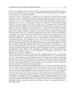
Fig. 10. FD-CMA Filter for frational time delay estimation and its corresponding path
detection.
The following subsections present the FTDE filter developed and adopted in this work, and
adaptive beamforming to estimate, the fractional delay and its corresponding path,
respectively.
A- Fractional Time Delay Estimation
Once the first path is estimated by the MCMA filter, it is delayed by an estimated value
using the fractional time delay filter H. This filtering is carried out by using the following
equation using ideal fractional-delay filter with sinc function interpolation:
∞
∞
, (41)
where the infinity sign in the summation is replaced by an integer P, which is chosen
sufficiently large to minimize the truncation error. is the instantaneous estimated time
delay. If is a fractional number, i.e. 0 < < 1, the sinc interpolation impulse response has
non-zero values for all n:
(42)
The delayed signal,
, is the output of the FIR filter H whose coefficients are
and input is
. For this issue, a lookup table of the sinc function is constructed that
consists of a matrix H of dimension K×(2P+1), with a generic element:
(43)
where K represents the inverse resolution over T
s
of the estimated delay . The theoretical
elements of the i-th row of the matrix H are therefore identical to the samples of the
truncated sinc function with delay equal to:
(44)
For the time delay estimation process, only the estimated time delay
is adapted in our
approach, and it is used as an index to obtain the vector h
i
from a lookup table. As
mentioned previously, this lookup table is a two-dimensional matrix called H of size
K×(2P+1) that contains samples of the sinc function with delay ranging from 0 to (K - 1)/K.
For a given vector with theoretically delayed value elements
given by (44), the i-th row
is computed as follows
. (45)
So, at each iteration, the integer part of
is used to locate the i-th row of the matrix
H, i.e. h
i
, that is used to delay the signal y
MCMA
(k) using
, (46)
where u(k) is given by:
(47)
The estimated fractional time delay is obtained by using the gradient descent of the
instantaneous squared error
surface to locate the global minimum, i.e., using LMS (So
et al., 1994). The estimated gradient is equal to the derivative of
with respect to . The
FTDE algorithm may be summarized as follows. The complex error signal,
, is given
by:
, (48)
where
(49)
. (50)
x
e1
(k) is delayed by (P +1). T
s
to be aligned with the output of the filter H, i.e., y
h
(k), that has
latency depending on its order value M = 2P + 1 as shown in Figure 10. The estimated time
delay can be adapted by minimizing the cost function given by:
. (51)
The constrained LMS algorithm becomes:
(52)
where
is a small positive step size.
By differentiating the instantaneous error surface,
, with respect to the estimated time
delay, we have:
MobileandWirelessCommunications:Physicallayerdevelopmentandimplementation92
(53)
where
(54)
Finally, the estimated time delay is given by:
. (55)
In our implementation, lookup tables of cos and sinc functions are constructed for different
values of and used to calculate . At each iteration, the integer part of
is used to locate the i-th row of the matrix H, i.e.
that is used to delay the signal
by the estimated fractional delay using (46).
B- Beamforming for fractional-delay path extraction
Now to extract the fractional-delay path, the weight vector of the FD-CMA filter is adapted
using LMS by minimizing the cost function given in (51) as follows:
, (56)
where
is a small positive step size.
5. General SBB Approach
According to statistical modeling presented in (Boutin et al., 2008) of the studied
underground channel, we were able to characterize, among many other channel parameters,
the maximum number of paths at a given operation frequency and a given path resolution.
Thus, we can assume for a given transmission rate and modulation type that the maximum
number of paths arriving with delays that are a multiple integer of the sampling interval as
well as the maximum number of paths arriving with fractional time delays are both
predicted accurately. Consequently, we assume n paths causing ISI and p paths causing isi.
In this general case of the presence of paths arriving with integer and fractional delay
multiples of the sampling intervals, the two ID-CMA SBB and FD-CMA SBB proposed
methods can be combined in a single approach named here as General Sequential Blind
Beamforming (G-SBB) approach.
To simplify, the following study is performed using a three-path channel model for
illustration purposes where the TPAs are given by
1
= 0 (the strongest path),
2
= < T
s
, and
3
= T
s
. Hence the received signal at the m-th antenna can be expressed by:
. (57)
Figure 11 depicts the new approach using sequential blind spatial-domain path-diversity
beamforming (SBB) to remedy both the ISI and isi problems using jointly CMA, LMS and
adaptive FTDE filtering. This approach is designed to sequentially recover multipath rays
by using multiple beamformings for received power maximization. First, the strongest path
is extracted using the MCMA (AitFares et al., 2004; AitFares et al., 2006 a; AitFares et al.,
2006 b; AitFares et al., 2008). Second, the path coming with delay that is multiple integer of
the sampling interval is estimated using ID-CMA filter (i.e., y
ID
) adapted using LMS with the
CMA delayed output as a reference signal (AitFares et al., 2004). Finally, the path coming
with fractional delay is estimated using FD-CMA filter (i.e., y
FD
) (AitFares et al., 2006 a)
adapted using LMS and FTDE. However, in order to ensure the estimated path arriving
with the fractional delay, two ASC filters are used to extract the contribution of path
y
MCMA
(k) and y
ID
(k) from the received signal vector x(k). As for the estimated path
combination, we propose in the next section a combination based on MRC.
Fig. 11. Proposed G-SBB approach.
6. MRC Path Combination
The paths y
MCMA
, y
FD
and y
ID
, estimated by the filters MCMA, FD-CMA and ID-CMA,
respectively, possess a common phase ambiguity, since they are sequentially extracted using
y
MCMA
as a reference signal. As a result, a combination based on a simple addition of the
estimated paths can only be constructive and it represents the output of a coherent Equal
Gain Combiner (EGC) as illustrated in Figure 12(a). After appropriate delay alignments, the
final estimated signal is given by EGC combining of the extracted paths as follows:
ݕ
ሺ
݇
ሻ
ൌݕ
ெெ
ሺ
݇
ሻ
ݕ
ி
ሺ
݇
ሻ
ݕ
ூ
ሺ
݇ͳ
ሻ
. (58)
For a Differential Binary Phase Shift Keying (DBPSK) modulation scheme, where the
common phase ambiguity is actually a sign ambiguity, an EGC is equivalent to MRC.
SequentialBlindBeamformingforWirelessMultipathCommunicationsinConnedAreas 93
(53)
where
(54)
Finally, the estimated time delay is given by:
. (55)
In our implementation, lookup tables of cos and sinc functions are constructed for different
values of and used to calculate . At each iteration, the integer part of
is used to locate the i-th row of the matrix H, i.e.
that is used to delay the signal
by the estimated fractional delay using (46).
B- Beamforming for fractional-delay path extraction
Now to extract the fractional-delay path, the weight vector of the FD-CMA filter is adapted
using LMS by minimizing the cost function given in (51) as follows:
, (56)
where
is a small positive step size.
5. General SBB Approach
According to statistical modeling presented in (Boutin et al., 2008) of the studied
underground channel, we were able to characterize, among many other channel parameters,
the maximum number of paths at a given operation frequency and a given path resolution.
Thus, we can assume for a given transmission rate and modulation type that the maximum
number of paths arriving with delays that are a multiple integer of the sampling interval as
well as the maximum number of paths arriving with fractional time delays are both
predicted accurately. Consequently, we assume n paths causing ISI and p paths causing isi.
In this general case of the presence of paths arriving with integer and fractional delay
multiples of the sampling intervals, the two ID-CMA SBB and FD-CMA SBB proposed
methods can be combined in a single approach named here as General Sequential Blind
Beamforming (G-SBB) approach.
To simplify, the following study is performed using a three-path channel model for
illustration purposes where the TPAs are given by
1
= 0 (the strongest path),
2
= < T
s
, and
3
= T
s
. Hence the received signal at the m-th antenna can be expressed by:
. (57)
Figure 11 depicts the new approach using sequential blind spatial-domain path-diversity
beamforming (SBB) to remedy both the ISI and isi problems using jointly CMA, LMS and
adaptive FTDE filtering. This approach is designed to sequentially recover multipath rays
by using multiple beamformings for received power maximization. First, the strongest path
is extracted using the MCMA (AitFares et al., 2004; AitFares et al., 2006 a; AitFares et al.,
2006 b; AitFares et al., 2008). Second, the path coming with delay that is multiple integer of
the sampling interval is estimated using ID-CMA filter (i.e., y
ID
) adapted using LMS with the
CMA delayed output as a reference signal (AitFares et al., 2004). Finally, the path coming
with fractional delay is estimated using FD-CMA filter (i.e., y
FD
) (AitFares et al., 2006 a)
adapted using LMS and FTDE. However, in order to ensure the estimated path arriving
with the fractional delay, two ASC filters are used to extract the contribution of path
y
MCMA
(k) and y
ID
(k) from the received signal vector x(k). As for the estimated path
combination, we propose in the next section a combination based on MRC.
Fig. 11. Proposed G-SBB approach.
6. MRC Path Combination
The paths y
MCMA
, y
FD
and y
ID
, estimated by the filters MCMA, FD-CMA and ID-CMA,
respectively, possess a common phase ambiguity, since they are sequentially extracted using
y
MCMA
as a reference signal. As a result, a combination based on a simple addition of the
estimated paths can only be constructive and it represents the output of a coherent Equal
Gain Combiner (EGC) as illustrated in Figure 12(a). After appropriate delay alignments, the
final estimated signal is given by EGC combining of the extracted paths as follows:
ݕ
ሺ
݇
ሻ
ൌݕ
ெெ
ሺ
݇
ሻ
ݕ
ி
ሺ
݇
ሻ
ݕ
ூ
ሺ
݇ͳ
ሻ
. (58)
For a Differential Binary Phase Shift Keying (DBPSK) modulation scheme, where the
common phase ambiguity is actually a sign ambiguity, an EGC is equivalent to MRC.
MobileandWirelessCommunications:Physicallayerdevelopmentandimplementation94
However, for higher order modulations such as Differential Quadrature Phase Shift Keying
(DQPSK), where the common phase ambiguity is an unknown angular rotation, more
substantial improvement compared to EGC can be obtained by implementing coherent
MRC with hard DFI as shown in Figure 12(b), which strives to force this common phase
ambiguity to known quantized values that keep the constellation invariant by rotation
(Affes & Mermelstein, 2003), thereby allowing coherent demodulation and MRC detection.
In the first step, all paths y
MCMA
, y
FD
and y
ID
are aligned by appropriate additional delays,
and then scaled by an MRC weighting vector g(k). The summation of these scaled paths,
, is given by
, (59)
where
, (60)
. (61)
In the next step,
, is quantized by making a hard decision to match it to a tentative
symbol
. This coherent-detection operation can be expressed as follows:
, (62)
where A
M
represents the MPSK modulation constellation defined by:
(63)
Since
provides a selected estimate of the desired signal, it can be used as a feedback
reference signal to update the weight vector g(k) using LMS-type adaptation referred to as
Decision Feedback Identification (DFI):
(64)
where
is a small positive step size.
Fig. 12. Path diversity combining stage for the SBB using EGC or Coherent MRC with hard
DFI.
It is this DFI procedure that enables coherent MRC detection by forcing the common phase
ambiguity of the extracted paths to a value by which the constellation is invariant by
rotation
(Affes & Mermelstein, 2003; Aitfares et al., 2008). Finally the desired output signal
y(k) is estimated from
by differential decoding, as shown in Figure 12(b), instead of
differential demodulation needed previously with simple EGC. This final decoding step is
expressed by:
. (65)
The proposed SBB technique enabling MRC path diversity combining (i.e., MRC-SBB) offers
an SNR gain of about 2 dB gain compared to that using simple EGC implementation (i.e.,
EGC-SBB) (Affes & Mermelstein, 2003; Aitfares et al., 2008).
7. Computer simulation results
In this section, simulation results are presented to assess the performance of the proposed
SBB method and to compare it with MCMA beamforming (Oh & Chin, 1995). A two-element
array with half-wavelength spacing is considered. A desired signal is propagated along four
multipaths to the antenna array while the interference and noise are simulated as additive
white Gaussian noise. The first path is direct with a path arrival-time delay
1
= 0. The
second and third paths arrive, respectively, with delays
2
and
3
lower than the sampling
interval, and the last path arrives with delay
4
= T
s
. Differential encoding is employed to
overcome the phase ambiguity in the signal estimation. Performance study was carried out
with two channel models and for two kinds of modulation (DBPSK and DQPSK). Type-A
channel is Rayleigh fading with a Doppler shift f
d1
= 20 Hz. Type-B channel is Rayleigh
fading with a higher Doppler shift f
d2
= 35 Hz. The use of these two Doppler frequencies
reflects the typical range of the vehicle speed in underground environments
2
. The Bit Error
Rate (BER) performance for different Doppler frequencies (f
d1
and f
d2
) was also studied. The
figure of merit is the required SNR to achieve a BER
3
below 0.001. Table 1 summarizes the
system parameters for the computer simulations.
2
For operations at a carrier frequency f
c
= 2:4 GHz and vehicle speeds v
1
= 10km=h, and v
2
= 15km=h, we
found approximately that f
d
1
=20 Hz and f
d
2
= 35Hz.
3
The BER is calculated after steady-state convergence to avoid biasing the results.
SequentialBlindBeamformingforWirelessMultipathCommunicationsinConnedAreas 95
However, for higher order modulations such as Differential Quadrature Phase Shift Keying
(DQPSK), where the common phase ambiguity is an unknown angular rotation, more
substantial improvement compared to EGC can be obtained by implementing coherent
MRC with hard DFI as shown in Figure 12(b), which strives to force this common phase
ambiguity to known quantized values that keep the constellation invariant by rotation
(Affes & Mermelstein, 2003), thereby allowing coherent demodulation and MRC detection.
In the first step, all paths y
MCMA
, y
FD
and y
ID
are aligned by appropriate additional delays,
and then scaled by an MRC weighting vector g(k). The summation of these scaled paths,
, is given by
, (59)
where
, (60)
. (61)
In the next step,
, is quantized by making a hard decision to match it to a tentative
symbol
. This coherent-detection operation can be expressed as follows:
, (62)
where A
M
represents the MPSK modulation constellation defined by:
(63)
Since
provides a selected estimate of the desired signal, it can be used as a feedback
reference signal to update the weight vector g(k) using LMS-type adaptation referred to as
Decision Feedback Identification (DFI):
(64)
where
is a small positive step size.
Fig. 12. Path diversity combining stage for the SBB using EGC or Coherent MRC with hard
DFI.
It is this DFI procedure that enables coherent MRC detection by forcing the common phase
ambiguity of the extracted paths to a value by which the constellation is invariant by
rotation
(Affes & Mermelstein, 2003; Aitfares et al., 2008). Finally the desired output signal
y(k) is estimated from
by differential decoding, as shown in Figure 12(b), instead of
differential demodulation needed previously with simple EGC. This final decoding step is
expressed by:
. (65)
The proposed SBB technique enabling MRC path diversity combining (i.e., MRC-SBB) offers
an SNR gain of about 2 dB gain compared to that using simple EGC implementation (i.e.,
EGC-SBB) (Affes & Mermelstein, 2003; Aitfares et al., 2008).
7. Computer simulation results
In this section, simulation results are presented to assess the performance of the proposed
SBB method and to compare it with MCMA beamforming (Oh & Chin, 1995). A two-element
array with half-wavelength spacing is considered. A desired signal is propagated along four
multipaths to the antenna array while the interference and noise are simulated as additive
white Gaussian noise. The first path is direct with a path arrival-time delay
1
= 0. The
second and third paths arrive, respectively, with delays
2
and
3
lower than the sampling
interval, and the last path arrives with delay
4
= T
s
. Differential encoding is employed to
overcome the phase ambiguity in the signal estimation. Performance study was carried out
with two channel models and for two kinds of modulation (DBPSK and DQPSK). Type-A
channel is Rayleigh fading with a Doppler shift f
d1
= 20 Hz. Type-B channel is Rayleigh
fading with a higher Doppler shift f
d2
= 35 Hz. The use of these two Doppler frequencies
reflects the typical range of the vehicle speed in underground environments
2
. The Bit Error
Rate (BER) performance for different Doppler frequencies (f
d1
and f
d2
) was also studied. The
figure of merit is the required SNR to achieve a BER
3
below 0.001. Table 1 summarizes the
system parameters for the computer simulations.
2
For operations at a carrier frequency f
c
= 2:4 GHz and vehicle speeds v
1
= 10km=h, and v
2
= 15km=h, we
found approximately that f
d
1
=20 Hz and f
d
2
= 35Hz.
3
The BER is calculated after steady-state convergence to avoid biasing the results.
MobileandWirelessCommunications:Physicallayerdevelopmentandimplementation96
Modulation DBPSK or DQPSK.
Antenna array type Linear uniform, with λ/2 element spacing.
Antenna array size 2 elements or 4 elements.
Max. Doppler frequency f
d1
=20Hz and f
d2
=35Hz.
Channel model Type-A: Rayleigh fading with f
d1
Type-B: Rayleigh fading with f
d2
Adaptive algorithm CMA & LMS
Carrier Frequency f
c
=2.4GHz
Noise AWGN
Filter order M=21
Path resolution K =200, i.e. T
r
=0.005 T
s
Step sizes μ=0.009; μ
1
= 0.008; μ
2
=0.0095; μ
3
=0.008;
μ
4
= 0.001; μ
5
= 0.009 and μ
6
= 0.001.
Number of symbol 10.000
Table 1. Simulation parameters.
Figs. 13 and 14 show the measured BER performance versus SNR of G-SBB and MCMA for
Type-A and -B channels, with different values of ߬
2
and ߬
3
using a DBPSK modulated signal.
As expected, it can be noted that for both algorithms, the BER performance decreases with
increasing Doppler frequency values. Despite the speed increasing due to the Doppler
effect, the proposed algorithm G-SSB provides significant gains and outperforms MCMA by
approximately 5 dB for both channel environments (A and B).
Fig. 13. BER performance versus SNR with ߬
2
=0.4T
s
and ߬
3
= 0.8T
s
for DBPSK modulation
scheme using a 2-element antenna array.
-4 -2 0 2 4 6 8 10 12
10
-4
10
-3
10
-2
10
-1
10
0
BER
SNR
G-SBB, T ype –A Channel
MCMA, Type –A Channel
G-SBB, T ype –B Channel
MCMA, Type –B Channel
Fig. 14. BER performance versus SNR with ߬
2
=0.3T
s
and ߬
3
= 0.7T
s
for DBPSK modulation
scheme using a 2-element antenna array.
Let us now study the convergence rate of the proposed G-SBB method compared to the
MCMA algorithm for the Type-A channel with ߬
2
= 0.4 T
s
and ߬
3
= 0.8 T
s
at 2.4 GHz and for
SNR = 4 dB. Figure 15 illustrates the average BER in terms of the number of iterations for the
first 8000 samples. A benchmark comparison with AAA using the LMS algorithm is also
provided. From Figure 15, it can be seen that the LMS algorithm is the fastest one followed
by the MCMA and than the G-SBB algorithms. However, the proposed G-SBB algorithm
reaches a much lower steady-state BER after convergence within a shorter delay compared
to AAA and MCMA.
Fig. 15. The real-time performance of the proposed system compared with the MCMA and LMS
algorithms at SNR = 4 dB for DBPSK modulation scheme using a 2-element antenna array.
-4 -2 0 2 4 6 8 10 12
10
-4
10
-3
10
-2
10
-1
10
0
SNR
BER
G-SBB, T ype –A Channel
MCMA, Type –A Channel
G-SBB, T ype –B Channel
MCMA, Type –B Channel
0 1000 2000 3000 4000 5000 6000 7000 8000
10
-3
10
-2
10
-1
10
0
Symbol Number
Average BER
SBB
LMS
MCMA
SequentialBlindBeamformingforWirelessMultipathCommunicationsinConnedAreas 97
Modulation DBPSK or DQPSK.
Antenna array type Linear uniform, with λ/2 element spacing.
Antenna array size 2 elements or 4 elements.
Max. Doppler frequency f
d1
=20Hz and f
d2
=35Hz.
Channel model Type-A: Rayleigh fading with f
d1
Type-B: Rayleigh fading with f
d2
Adaptive algorithm CMA & LMS
Carrier Frequency f
c
=2.4GHz
Noise AWGN
Filter order M=21
Path resolution K =200, i.e. T
r
=0.005 T
s
Step sizes μ=0.009; μ
1
= 0.008; μ
2
=0.0095; μ
3
=0.008;
μ
4
= 0.001; μ
5
= 0.009 and μ
6
= 0.001.
Number of symbol 10.000
Table 1. Simulation parameters.
Figs. 13 and 14 show the measured BER performance versus SNR of G-SBB and MCMA for
Type-A and -B channels, with different values of ߬
2
and ߬
3
using a DBPSK modulated signal.
As expected, it can be noted that for both algorithms, the BER performance decreases with
increasing Doppler frequency values. Despite the speed increasing due to the Doppler
effect, the proposed algorithm G-SSB provides significant gains and outperforms MCMA by
approximately 5 dB for both channel environments (A and B).
Fig. 13. BER performance versus SNR with ߬
2
=0.4T
s
and ߬
3
= 0.8T
s
for DBPSK modulation
scheme using a 2-element antenna array.
-4 -2 0 2 4 6 8 10 12
10
-4
10
-3
10
-2
10
-1
10
0
BER
SNR
G-SBB, T ype –A Channel
MCMA, Type –A Channel
G-SBB, T ype –B Channel
MCMA, Type –B Channel
Fig. 14. BER performance versus SNR with ߬
2
=0.3T
s
and ߬
3
= 0.7T
s
for DBPSK modulation
scheme using a 2-element antenna array.
Let us now study the convergence rate of the proposed G-SBB method compared to the
MCMA algorithm for the Type-A channel with ߬
2
= 0.4 T
s
and ߬
3
= 0.8 T
s
at 2.4 GHz and for
SNR = 4 dB. Figure 15 illustrates the average BER in terms of the number of iterations for the
first 8000 samples. A benchmark comparison with AAA using the LMS algorithm is also
provided. From Figure 15, it can be seen that the LMS algorithm is the fastest one followed
by the MCMA and than the G-SBB algorithms. However, the proposed G-SBB algorithm
reaches a much lower steady-state BER after convergence within a shorter delay compared
to AAA and MCMA.
Fig. 15. The real-time performance of the proposed system compared with the MCMA and LMS
algorithms at SNR = 4 dB for DBPSK modulation scheme using a 2-element antenna array.
-4 -2 0 2 4 6 8 10 12
10
-4
10
-3
10
-2
10
-1
10
0
SNR
BER
G-SBB, T ype –A Channel
MCMA, Type –A Channel
G-SBB, T ype –B Channel
MCMA, Type –B Channel
0 1000 2000 3000 4000 5000 6000 7000 8000
10
-3
10
-2
10
-1
10
0
Symbol Number
Average BER
SBB
LMS
MCMA
MobileandWirelessCommunications:Physicallayerdevelopmentandimplementation98
Here we discuss the trade-off between the hardware complexity related to the delay
resolution implementation and the BER performance. As mentioned above, K, given in
equation (44), represents the number of the tap filter coefficients used to implement the
fractional delay resolution. For instance, when K = 10, the delay resolution is equal to
T
r
=1/(K.T
s
) = 0.1 T
s
. By increasing the value of K, we increase the FTDE resolution and
consequently the FTDE filter will be able to estimate faithfully the fractional delay path
which will in turn improve the BER performance. On the other hand, increasing K increases
the hardware complexity needed to implement the FTDE. To find an optimal trade-off
between resolution and hardware complexity, several simulations with different values of K
in terms of BER performance were conducted.
Figure 16 illustrates the simulated BER performance versus SNR of the G-SBB for Type-A
channel environment at different values of T
r
. From this figure, it can be seen that the
resolution of K impacts greatly the BER performance when K is less than 50. For K greater
than 50, the optimal performance is attained and further increase of the K value is
unnecessary.
Fig. 16. BER performance versus SNR in Type -A Channel for ߬
2
= 0.4T
s
and ߬
3
= 0.8T
s
when
T
r
is varied using a 2-element antenna array.
For high order modulation using DQPSK, Figs. 17 and 18 illustrate the BER performance
versus SNR for G-SBB using MRC or EGC in the combining step for Type-A and –B channels
with ߬
2
= 0.4 T
s
and ߬
3
= 0.8 T
s
, respectively, at 2.4 GHz. A benchmark comparison with AAA
using MCMA is also provided. For the type-A channel, the results show that G-SBB with
MRC provides a good enhancement and outperforms G-SBB with EGC and the AAA using
MCMA by approximately 2 dB and up to 7 dB at a required BER =0.001, respectively (Figure
17). For the type- B channel with higher Doppler frequency, the measured results show that
G-SBB with MRC maintains its advantage compared to G-SBB with EGC and to the AAA
using MCMA where improvements of approximately 2 dB and up to 7 dB at a required
BER=0.001 are obtained, respectively (Figure 18).
-4 -2 0 2 4 6 8 10 12 14 16
10
-4
10
-3
10
-2
10
-1
SNR
BER
G-SBB, T
r
=0.005T
s
G-SBB, T
r
=0.01T
s
G-SBB, T
r
=0.02T
s
G-SBB, T
r
=0.1T
s
M-CMA
Fig. 17. BER performance versus SNR for Type -A Channel with ߬
2
=0.4T
s
and ߬
3
= 0.8T
s
for
DQPSK modulation scheme using a 2-element antenna array.
Fig. 18. BER performance versus SNR for Type -B Channel with ߬
2
=0.4T
s
and ߬
3
= 0.8T
s
for
DQPSK modulation scheme using a 2-element antenna array.
Figure 19 shows the measured BER performance versus SNR for G-SBB using MRC or EGC
in the combining step and with MCMA-AAA for Type-A channel using four antenna
elements (N = 4). Again, it is clear that the G-SBB using the proposed MRC is more efficient
than both previous G-SBB versions using EGC and the conventional MCMA algorithm.
-6 -4 -2 0 2 4 6 8 10 12 14 16
10
-4
10
-3
10
-2
10
-1
SNR
BER
G-SBB-MRC
G-SBB-EGC
M-CMA
-6 -4 -2 0 2 4 6 8 10 12 14 16
10
-4
10
-3
10
-2
10
-1
SNR
BER
G-SBB-MRC
G-SBB-EGC
M-CMA
SequentialBlindBeamformingforWirelessMultipathCommunicationsinConnedAreas 99
Here we discuss the trade-off between the hardware complexity related to the delay
resolution implementation and the BER performance. As mentioned above, K, given in
equation (44), represents the number of the tap filter coefficients used to implement the
fractional delay resolution. For instance, when K = 10, the delay resolution is equal to
T
r
=1/(K.T
s
) = 0.1 T
s
. By increasing the value of K, we increase the FTDE resolution and
consequently the FTDE filter will be able to estimate faithfully the fractional delay path
which will in turn improve the BER performance. On the other hand, increasing K increases
the hardware complexity needed to implement the FTDE. To find an optimal trade-off
between resolution and hardware complexity, several simulations with different values of K
in terms of BER performance were conducted.
Figure 16 illustrates the simulated BER performance versus SNR of the G-SBB for Type-A
channel environment at different values of T
r
. From this figure, it can be seen that the
resolution of K impacts greatly the BER performance when K is less than 50. For K greater
than 50, the optimal performance is attained and further increase of the K value is
unnecessary.
Fig. 16. BER performance versus SNR in Type -A Channel for ߬
2
= 0.4T
s
and ߬
3
= 0.8T
s
when
T
r
is varied using a 2-element antenna array.
For high order modulation using DQPSK, Figs. 17 and 18 illustrate the BER performance
versus SNR for G-SBB using MRC or EGC in the combining step for Type-A and –B channels
with ߬
2
= 0.4 T
s
and ߬
3
= 0.8 T
s
, respectively, at 2.4 GHz. A benchmark comparison with AAA
using MCMA is also provided. For the type-A channel, the results show that G-SBB with
MRC provides a good enhancement and outperforms G-SBB with EGC and the AAA using
MCMA by approximately 2 dB and up to 7 dB at a required BER =0.001, respectively (Figure
17). For the type- B channel with higher Doppler frequency, the measured results show that
G-SBB with MRC maintains its advantage compared to G-SBB with EGC and to the AAA
using MCMA where improvements of approximately 2 dB and up to 7 dB at a required
BER=0.001 are obtained, respectively (Figure 18).
-4 -2 0 2 4 6 8 10 12 14 16
10
-4
10
-3
10
-2
10
-1
SNR
BER
G-SBB, T
r
=0.005T
s
G-SBB, T
r
=0.01T
s
G-SBB, T
r
=0.02T
s
G-SBB, T
r
=0.1T
s
M-CMA
Fig. 17. BER performance versus SNR for Type -A Channel with ߬
2
=0.4T
s
and ߬
3
= 0.8T
s
for
DQPSK modulation scheme using a 2-element antenna array.
Fig. 18. BER performance versus SNR for Type -B Channel with ߬
2
=0.4T
s
and ߬
3
= 0.8T
s
for
DQPSK modulation scheme using a 2-element antenna array.
Figure 19 shows the measured BER performance versus SNR for G-SBB using MRC or EGC
in the combining step and with MCMA-AAA for Type-A channel using four antenna
elements (N = 4). Again, it is clear that the G-SBB using the proposed MRC is more efficient
than both previous G-SBB versions using EGC and the conventional MCMA algorithm.
-6 -4 -2 0 2 4 6 8 10 12 14 16
10
-4
10
-3
10
-2
10
-1
SNR
BER
G-SBB-MRC
G-SBB-EGC
M-CMA
-6 -4 -2 0 2 4 6 8 10 12 14 16
10
-4
10
-3
10
-2
10
-1
SNR
BER
G-SBB-MRC
G-SBB-EGC
M-CMA
MobileandWirelessCommunications:Physicallayerdevelopmentandimplementation100
Fig. 19. BER performance versus SNR for Type -A Channel with ߬
2
=0.2T
s
and ߬
3
= 0.8T
s
for
DQPSK modulation scheme using a 4-element antenna array.
8. Conclusion
In this Chapter, a new approach using sequential blind spatial-domain path-diversity
beamforming (SBB) to remedy the ISI and isi problems has been presented. Using jointly
CMA, LMS and adaptive FTDE filtering, this approach has been designed to sequentially
recover multipath rays to maximize the received power by extracting all dominant
multipaths. MCMA is used to estimate the strongest path while the integer path delay is
estimated sequentially using adapted LMS with the first beamformer output as a reference
signal. A new synchronization approach for multipath propagation, based on combining a
CMA-AAA and adaptive fractional time delay estimation filtering, has been proposed to
estimate the fractional path delay. It should be noted that the G-SBB architecture can be
generalized for an arbitrary number of received paths causing ISI where several concurrent
filters (ID-CMA and FD-CMA) can be implemented to resolve the different paths. Finally, to
combine these extracted paths, an enabling MRC path diversity combiner with hard DFI has
also been proposed. Simulation results show the effectiveness of the proposed SBB receiver
especially at high SNR, where it is expected to operate in a typical underground wireless
environment (Nerguizian et al., 2005).
-6 -4 -2 0 2 4 6 8 10 12 14
10
-4
10
-3
10
-2
10
-1
10
0
SNR
BER
G-SBB -MRC
G-SBB-EGC
M-CMA
9. References
AitFares, S.; Denidni, T. A. & Affes, S. (2004). Sequential blind beamforming algorithm using
combined CMA/LMS for wireless underground communications, in Proc. IEEE
VTC’04, vol. 5, pp. 3600-3604, Sept. 2004.
AitFares, S; Denidni, T. A.; Affes, S. & Despins, C. (2006). CMA/fractional delay sequential
blind beamforming for wireless multipath communications, in Proc. IEEE VTC’06,
vol. 6, pp. 2793-2797, May 2006.
AitFares, S; Denidni, T. A.; Affes, S. & Despins, C. (2006). Efficient sequential blind
beamforming for wireless underground communications, in Proc. IEEE VTC’06, pp.
1-4, Sept. 2006.
AitFares, S; Denidni, T. A.; Affes, S. & Despins, C. (2008). Fractional-Delay Sequential Blind
Beamforming for Wireless Multipath Communications in Confined Areas. IEEE
Transactions on Wireless Communications, vol. 7, no. 1, pp. 1-10, January 2008.
Affes, S. & Mermelstein, P. (2003). Adaptive space-time processing for wireless CDMA,
chapter 10, pp. 283-321, in Adaptive Signal Processing: Application to Real-World
Problems, J. Benesty and A. H. Huang, eds. Berlin: Springer, 2003.
Amca, H.; Yenal, T. & Hacioglu, K. (1999). Adaptive equalization of frequency selective
multipath fading channels based on sample selection, Proc. IEE on Commun., vol.
146, no. 1, pp. 55-60, Feb. 1999.
Bellofiore, S.; Balanis, C. A.; Foutz, J. & Spanias, A. S. (2002). Smart antenna systems for
mobile communication networks, part 1: overview and antenna design, IEEE
Antennas Propag. Mag., vol. 44, no. 3, pp. 145-154, June 2002.
Bellofiore, S.; Foutz, J.; Balanis, C. A. & Spanias, A. S. (2002). Smart-antenna systems for
mobile communication networks, part 2: beamforming and network throughput,
IEEE Antennas Propagation Magazine, vol. 44, no. 4, pp. 106-114, Aug. 2002.
Boutin, M. ; Benzakour, A; Despins, C & Affes, S. (2008). Radio Wave Characterization and
Modeling in Underground Mine Tunnels, IEEE Transaction on Antennas and
Propagation, vol. 56, no. 2, pp. 540-549, February 2008.
Chao, R. Y. & Chung, K. S. (1994). A low profile antenna array for underground mine
communication, in Proc. ICCS 1994, vol. 2, pp. 705-709, 1994.
Cozzo, C. & Hughes, B. L. (2003). Space diversity in presence of discrete multipath fading
channel, IEEE Trans. Commun., vol. 51, no. 10, pp. 1629-1632, Oct. 2003.
Furukawa, H.; Kamio, Y. & Sasaoka, H. (1996). Co-Channel interference reduction method
using CMA adaptive array antenna, IEEE International Symposium on Personal,
Indoor and Mobile Radio Communications, vol. 2, pp. 512-516, 1996.
Godara, L. C. (1997). Applications of antenna arrays to mobile communications, part I:
performance improvement, feasibility, and system considerations, Proc. IEEE, vol.
85, no. 7, pp. 1031-1060, July 1997.
Lee, W. C. & Choi, S. (2005). Adaptive beamforming algorithm based on eigen-space method
for smart antennas, IEEE Commun. Lett., vol. 9, no. 10, pp. 888-890, Oct. 2005.
McNeil, D.; Denidni, A. T. & Delisle, G. Y. (2001). Output power maximization algorithm
performance of dual-antenna for personal communication handset applications, in
Proc. IEEE Antennas and Propagation Society International Symposium, vol. 1, pp. 128-
131, July 2001.
SequentialBlindBeamformingforWirelessMultipathCommunicationsinConnedAreas 101
Fig. 19. BER performance versus SNR for Type -A Channel with ߬
2
=0.2T
s
and ߬
3
= 0.8T
s
for
DQPSK modulation scheme using a 4-element antenna array.
8. Conclusion
In this Chapter, a new approach using sequential blind spatial-domain path-diversity
beamforming (SBB) to remedy the ISI and isi problems has been presented. Using jointly
CMA, LMS and adaptive FTDE filtering, this approach has been designed to sequentially
recover multipath rays to maximize the received power by extracting all dominant
multipaths. MCMA is used to estimate the strongest path while the integer path delay is
estimated sequentially using adapted LMS with the first beamformer output as a reference
signal. A new synchronization approach for multipath propagation, based on combining a
CMA-AAA and adaptive fractional time delay estimation filtering, has been proposed to
estimate the fractional path delay. It should be noted that the G-SBB architecture can be
generalized for an arbitrary number of received paths causing ISI where several concurrent
filters (ID-CMA and FD-CMA) can be implemented to resolve the different paths. Finally, to
combine these extracted paths, an enabling MRC path diversity combiner with hard DFI has
also been proposed. Simulation results show the effectiveness of the proposed SBB receiver
especially at high SNR, where it is expected to operate in a typical underground wireless
environment (Nerguizian et al., 2005).
-6 -4 -2 0 2 4 6 8 10 12 14
10
-4
10
-3
10
-2
10
-1
10
0
SNR
BER
G-SBB -MRC
G-SBB-EGC
M-CMA
9. References
AitFares, S.; Denidni, T. A. & Affes, S. (2004). Sequential blind beamforming algorithm using
combined CMA/LMS for wireless underground communications, in Proc. IEEE
VTC’04, vol. 5, pp. 3600-3604, Sept. 2004.
AitFares, S; Denidni, T. A.; Affes, S. & Despins, C. (2006). CMA/fractional delay sequential
blind beamforming for wireless multipath communications, in Proc. IEEE VTC’06,
vol. 6, pp. 2793-2797, May 2006.
AitFares, S; Denidni, T. A.; Affes, S. & Despins, C. (2006). Efficient sequential blind
beamforming for wireless underground communications, in Proc. IEEE VTC’06, pp.
1-4, Sept. 2006.
AitFares, S; Denidni, T. A.; Affes, S. & Despins, C. (2008). Fractional-Delay Sequential Blind
Beamforming for Wireless Multipath Communications in Confined Areas. IEEE
Transactions on Wireless Communications, vol. 7, no. 1, pp. 1-10, January 2008.
Affes, S. & Mermelstein, P. (2003). Adaptive space-time processing for wireless CDMA,
chapter 10, pp. 283-321, in Adaptive Signal Processing: Application to Real-World
Problems, J. Benesty and A. H. Huang, eds. Berlin: Springer, 2003.
Amca, H.; Yenal, T. & Hacioglu, K. (1999). Adaptive equalization of frequency selective
multipath fading channels based on sample selection, Proc. IEE on Commun., vol.
146, no. 1, pp. 55-60, Feb. 1999.
Bellofiore, S.; Balanis, C. A.; Foutz, J. & Spanias, A. S. (2002). Smart antenna systems for
mobile communication networks, part 1: overview and antenna design, IEEE
Antennas Propag. Mag., vol. 44, no. 3, pp. 145-154, June 2002.
Bellofiore, S.; Foutz, J.; Balanis, C. A. & Spanias, A. S. (2002). Smart-antenna systems for
mobile communication networks, part 2: beamforming and network throughput,
IEEE Antennas Propagation Magazine, vol. 44, no. 4, pp. 106-114, Aug. 2002.
Boutin, M. ; Benzakour, A; Despins, C & Affes, S. (2008). Radio Wave Characterization and
Modeling in Underground Mine Tunnels, IEEE Transaction on Antennas and
Propagation, vol. 56, no. 2, pp. 540-549, February 2008.
Chao, R. Y. & Chung, K. S. (1994). A low profile antenna array for underground mine
communication, in Proc. ICCS 1994, vol. 2, pp. 705-709, 1994.
Cozzo, C. & Hughes, B. L. (2003). Space diversity in presence of discrete multipath fading
channel, IEEE Trans. Commun., vol. 51, no. 10, pp. 1629-1632, Oct. 2003.
Furukawa, H.; Kamio, Y. & Sasaoka, H. (1996). Co-Channel interference reduction method
using CMA adaptive array antenna, IEEE International Symposium on Personal,
Indoor and Mobile Radio Communications, vol. 2, pp. 512-516, 1996.
Godara, L. C. (1997). Applications of antenna arrays to mobile communications, part I:
performance improvement, feasibility, and system considerations, Proc. IEEE, vol.
85, no. 7, pp. 1031-1060, July 1997.
Lee, W. C. & Choi, S. (2005). Adaptive beamforming algorithm based on eigen-space method
for smart antennas, IEEE Commun. Lett., vol. 9, no. 10, pp. 888-890, Oct. 2005.
McNeil, D.; Denidni, A. T. & Delisle, G. Y. (2001). Output power maximization algorithm
performance of dual-antenna for personal communication handset applications, in
Proc. IEEE Antennas and Propagation Society International Symposium, vol. 1, pp. 128-
131, July 2001.
MobileandWirelessCommunications:Physicallayerdevelopmentandimplementation102
Nerguizian, C.; Despins, C; Affes, S. & Djadel, M. (2005). Radio-channel characterization of
an underground mine at 2:4 GHz wireless communications, IEEE Trans. Wireless
Communication, vol. 4, no. 5, pp. 2441-2453, Sept. 2005.
Oh, K. N. & Chin, Y. O. (1995). New blind equalization techniques based on constant
modulus algorithm, in Proc. Global Telecommunications Conference, vol. 2, pp. 865-
869, Nov. 1995.
Ogawa, Y.; Fujishima, K. & Ohgane, T. (1999). Weighting factors in spatial domain path-
diversity using an adaptive antenna,” in Proc. IEEE VTC’99, vol. 3, pp. 2184-2188,
May 1999.
Sanada, Y. & Wang, Q. (1997). A co-channel interference cancellation technique using
orthogonal convolutional codes on multipath Rayleigh fading channel, IEEE Trans.
Veh. Technol., vol. 46, no. 1, pp. 114-128, Feb. 1997.
Saunders, S. R. (1999). Antenna and Propagation for Wireless Communication Systems.
Chichester, England: John Wiley & Sons, Ltd., 1999.
Slock, D. T. M. (1994). Blind joint equalization of multiple synchronous mobile users using
over sampling and/or multiple antennas, in Proc. IEEE Asilomar Conference on
Signals, Systems and Computers, vol. 2, pp. 1154-1158, 1994.
Stott, J. H. (2000). The how and why of COFDM, tutorial COFDM, BBC Research and
Development, 278-stott.pdf
.
So, H. C.; Ching, P. C. & Chan, Y. T. (1994). New algorithm for explicit adaptation of time
delay, IEEE Trans. Signal Processing, vol. 42, no. 7, pp. 1816-1820, July, 1994.
Tanabe, Y. et al. (2000), An adaptive antenna for spatial-domain path-diversity using a
super-resolution technique, in Proc. IEEE VTC’00, vol. 1, pp. 1-5, May 2000.
Tanaka, T. (1994). A study on multipath propagation characteristics for RAKE receiving
technique, in Proc. 5th IEEE International Symposium on Personal, Indoor and Mobile
Radio Communication, vol. 2, pp. 711- 714, Sept. 1994.
Valimaki, V. & Laakso, T. I. (2000). Principles of fractional delay filters,” in Proc. IEEE
ICASS, vol. 6, pp. 3870-3873, June 2000.
Widrow, B.; Mantey, P. E.; Griffiths, L. J. & Goode, B. B. (1967). Adaptive antenna systems,”
Proc. IEEE, vol. 55, no. 12, pp. 2143-2159, Dec. 1967.
Youna, W. S. & Un, C. K. (1994). Robust adaptive beamforming based on the eigen-structure
method, IEEE Trans. Signal Processing, vol. 42, no. 6, pp. 1543-1547, June 1994.
Yuan, J.T. & Tsai, K.D. (2005). Analysis of the multimodulus blind equalization algorithm in
QAM communication systems, IEEE Transactions on Communications, vol. 53, no.
9, pp. 1427-1431, 2005.
Space-TimeDiversityTechniquesforWCDMAHighAltitudePlatformSystems 103
Space-Time Diversity Techniques for WCDMA High Altitude Platform
Systems
AbbasMohammedandTommyHult
0
Space-Time Diversity Techniques
for WCDMA High Altitude Platform Systems
Abbas Mohammed
Blekinge Institute of Technology
Sweden
Tommy Hult
Lund University
Sweden
1. Introduction
Third generation mobile systems are gradually being deployed in many developed countries
in hotspot areas. However, owing to the amount of new infrastructures required, it will still
be some time before 3G is ubiquitous, especially in developing countries. One possible cost
effective solution for deployments in these areas is to use High Altitude Platforms (HAPs)
(Collela et al., 2000; Djuknic et al., 1997; Grace et al., 2001; 2005; Miura & Oodo, 2002; Park et
al., 2002; Steele, 1992; Thornton et al., 2001; Tozer & Grace, 2001) for delivering 3G (WCDMA)
communications services over a wide coverage area (Dovis et al., 2002; Falletti & Sellone,
2005; Foo et al., 2000; Masumura & Nakagawa, 2002; Vazquez et al., 2002). HAPs are either
airships or planes that will operate in the stratosphere, 17-22 km above the ground. This
unique position offers a significant link budget advantage compared with satellites and much
wider coverage area than conventional terrestrial cellular systems. Such platforms will have
a rapid roll-out capability and the ability to serve a large number of users, using considerably
less communications infrastructure than required by a terrestrial network (Steele, 1992). In
order to aid the eventual deployment of HAPs the ITU has allocated spectrum in the 3G bands
for HAPs (ITU, 2000a), as well as in the mm-wave bands for broadband services at around
48 GHz worldwide (ITU, 2000b) and 31/28 GHz for certain Asian countries (Oodo et al., 2002).
Spectrum reuse is important in all wireless communications systems. Cellular solutions for
HAPs have been examined in (El-Jabu, 2001; Thornton et al., 2003), specifically addressing the
antenna beam characteristics required to produce an efficient cellular structure on the ground,
and the effect of antenna sidelobe levels on channel reuse plans (Thornton et al., 2003). HAPs
will have relatively loose station-keeping characteristics compared with satellites, and the ef-
fects of platform drift on a cellular structure and the resulting inter-cell handover require-
ments have been investigated (Thornton et al., 2005). Cellular resource management strategies
have also been developed for HAP use (Grace et al., 2002).
Configurations of multiple HAPs can also reuse the spectrum. They can be used to deliver
contiguous coverage and must take into account coexistence requirements (Falletti & Sell-
one, 2005; Foo et al., 2000). A technique not widely known is their ability to serve the same
6
MobileandWirelessCommunications:Physicallayerdevelopmentandimplementation104
coverage area reusing the spectrum to allow capacity enhancement. Such a technique has al-
ready been examined for TDMA/FDMA systems (Chen et al., 2005; Grace et al., 2005; Liu et
al., 2005). In order to achieve the required reduction in interference needed to permit spec-
trum reuse, the highly directional user antenna is used to spatially discriminate between the
HAPs. The degree of bandwidth reuse and resulting capacity gain is dependent on several
factors, in particular the number of platforms and the user antenna sidelobe levels. An al-
ternative method of enhancement is to apply space-time diversity techniques, such as Single-
Input Multiple-Output (SIMO) receive diversity or Multiple-Input Multiple-Output (MIMO)
diversity, to improve the spectrum reuse in the multiple HAP scenario.
In the case of many 3G systems the user antenna is either omni-directional or at best low gain,
so in these cases it cannot be used to achieve the same effects. The purpose of this chapter is to
examine how the unique properties of a WCDMA system can be exploited in multiple HAP
uplink architectures to deliver both coverage and capacity enhancement (without the need for
the user antenna gain).
In addition to the spectral reuse benefits, there are three main benefits for a multiple HAP
architecture:
∙ The configuration also provides for incremental roll-out: initially only one HAP needs
to be deployed. As more capacity is required, further HAPs can be brought into service,
with new users served by the newly deployed HAPs.
∙ Multiple operators can be served from individual HAPs, without the need for compli-
cated coexistence criteria since the individual HAPs could reuse the same spectrum.
∙ HAPs will be payload power, volume and weight constrained, limiting the overall ca-
pacity delivered by each platform. Capacity densities can be increased with more HAPs.
Moreover, it may be more cost effective to use more lower capability HAPs (e.g., solar
powered planes), rather than one big HAP (e.g., solar powered airship), when covering
a large number of cells (Grace et al., 2006).
The chapter is organized as follows: in section 2 the multiple HAP scenario is explained.
The interference analysis is presented in section 3. In section 4 we examine the completely
overlapping coverage area case, different numbers of platforms, and simulation results show-
ing the achievable capacity enhancement are presented. Finally, conclusions are presented in
section 5.
2. Multiple HAP system setup
In this chapter we use a simple geometric positioning of the high altitude platforms to create
signal environments that can easily be compared and analyzed. In each constellation, the
HAPs are located with equal separation along a circular contour, as shown in figure 1.
The separation distance d
m
along the line from the vertical projection of the HAP on the
ground to the cell centre is varied from 70 km to zero (i.e., all the HAPs will be located on
top of each other in the latter case). All HAPs are assumed to be flying in the stratosphere at
an altitude of 20 km. The size of the coverage area assigned to each HAP is governed by the
shape of the base station antenna pattern. If we assume that we only have one cell per HAP,
then the coverage area is also synonymous with the total cell area of the HAP.
R
d
m
q
m
Fig. 1. An example of a system simulation setup with N = 2 HAPs with overlapping cells of
radius R. d
m
is the distance on the ground between the cell centre and the vertical projection
of the HAP on the ground and θ
m
is the elevation angle towards the HAP.
2.1 User Positioning Geometry
Each UE (User Equipment) is positioned inside the cell according to an independent uniform
random distribution over the cell coverage area with radius R, as shown in figure 2. The
position of each UE inside each cell is defined relative to the HAP base station that it is con-
nected to, and also relative to every other HAP borne base station. This is necessary in order
to evaluate the impact of interference between the different UE-HAP transmission paths.
BS 1
BS 2
BS 3
Cell boundary
Fig. 2. A plot showing a sample distribution of 150 UE, where 50 UE are assigned to each of
the three base stations (BS1, BS2 and BS3).
Space-TimeDiversityTechniquesforWCDMAHighAltitudePlatformSystems 105
coverage area reusing the spectrum to allow capacity enhancement. Such a technique has al-
ready been examined for TDMA/FDMA systems (Chen et al., 2005; Grace et al., 2005; Liu et
al., 2005). In order to achieve the required reduction in interference needed to permit spec-
trum reuse, the highly directional user antenna is used to spatially discriminate between the
HAPs. The degree of bandwidth reuse and resulting capacity gain is dependent on several
factors, in particular the number of platforms and the user antenna sidelobe levels. An al-
ternative method of enhancement is to apply space-time diversity techniques, such as Single-
Input Multiple-Output (SIMO) receive diversity or Multiple-Input Multiple-Output (MIMO)
diversity, to improve the spectrum reuse in the multiple HAP scenario.
In the case of many 3G systems the user antenna is either omni-directional or at best low gain,
so in these cases it cannot be used to achieve the same effects. The purpose of this chapter is to
examine how the unique properties of a WCDMA system can be exploited in multiple HAP
uplink architectures to deliver both coverage and capacity enhancement (without the need for
the user antenna gain).
In addition to the spectral reuse benefits, there are three main benefits for a multiple HAP
architecture:
∙ The configuration also provides for incremental roll-out: initially only one HAP needs
to be deployed. As more capacity is required, further HAPs can be brought into service,
with new users served by the newly deployed HAPs.
∙ Multiple operators can be served from individual HAPs, without the need for compli-
cated coexistence criteria since the individual HAPs could reuse the same spectrum.
∙ HAPs will be payload power, volume and weight constrained, limiting the overall ca-
pacity delivered by each platform. Capacity densities can be increased with more HAPs.
Moreover, it may be more cost effective to use more lower capability HAPs (e.g., solar
powered planes), rather than one big HAP (e.g., solar powered airship), when covering
a large number of cells (Grace et al., 2006).
The chapter is organized as follows: in section 2 the multiple HAP scenario is explained.
The interference analysis is presented in section 3. In section 4 we examine the completely
overlapping coverage area case, different numbers of platforms, and simulation results show-
ing the achievable capacity enhancement are presented. Finally, conclusions are presented in
section 5.
2. Multiple HAP system setup
In this chapter we use a simple geometric positioning of the high altitude platforms to create
signal environments that can easily be compared and analyzed. In each constellation, the
HAPs are located with equal separation along a circular contour, as shown in figure 1.
The separation distance d
m
along the line from the vertical projection of the HAP on the
ground to the cell centre is varied from 70 km to zero (i.e., all the HAPs will be located on
top of each other in the latter case). All HAPs are assumed to be flying in the stratosphere at
an altitude of 20 km. The size of the coverage area assigned to each HAP is governed by the
shape of the base station antenna pattern. If we assume that we only have one cell per HAP,
then the coverage area is also synonymous with the total cell area of the HAP.
R
d
m
q
m
Fig. 1. An example of a system simulation setup with N = 2 HAPs with overlapping cells of
radius R. d
m
is the distance on the ground between the cell centre and the vertical projection
of the HAP on the ground and θ
m
is the elevation angle towards the HAP.
2.1 User Positioning Geometry
Each UE (User Equipment) is positioned inside the cell according to an independent uniform
random distribution over the cell coverage area with radius R, as shown in figure 2. The
position of each UE inside each cell is defined relative to the HAP base station that it is con-
nected to, and also relative to every other HAP borne base station. This is necessary in order
to evaluate the impact of interference between the different UE-HAP transmission paths.
BS 1
BS 2
BS 3
Cell boundary
Fig. 2. A plot showing a sample distribution of 150 UE, where 50 UE are assigned to each of
the three base stations (BS1, BS2 and BS3).
MobileandWirelessCommunications:Physicallayerdevelopmentandimplementation106
2.2 Base station antenna pattern
The base station antenna pattern for the simulations were chosen to be simple but detailed
enough to show the effects of the main and side lobes, especially in the null directions, as
illustrated in figure 3. A simple rotationally symmetric pattern based on a Bessel function is
used for this purpose, and is defined by (Balanis, 1997)
G
(ϕ) ≈ 0.7 ⋅
2
⋅ J
1
70π
ϕ
3dB
sin(ϕ)
sin(ϕ)
2
, (1)
where J
1
(⋅) is a Bessel function of the first kind and order 1, ϕ
3dB
is the 3 dB beamwidth in
degrees of the main antenna lobe. The 3 dB beamwidth of the antenna is computed from the
desired cell radius according to
ϕ
3dB
= 2 ⋅arctan
cell radius
HAP altitude
. (2)
Fig. 3. HAP base station antenna patterns for different cell radii.
2.3 User equipment antenna pattern
In this analysis we assume that each UE employs a directive antenna and communicates with
its corresponding HAP basestation. Using this assumption we only need to set the desired
maximum gain of the UE antenna we want to use, as shown Table 1. The antenna pattern of
the directive antennas is calculated according to equation (1), but with a fixed maximum gain
instead of a fixed main beamwidth, the beamwidth is then ϕ
(G
max
).
User Equipment Max. ant. Gain [dBi]
Mobile phone 0
Data terminal 2,4,12
Table 1. Antenna gains used in the simulation setup.
2.4 UE-HAP radio propagation channel model
In this chapter we use the Combined Empirical Fading Model (CEFM) together with the Free
Space Loss (FSL) model. CEFM combines the results of the Empirical Roadside Shadowing
(ERS) model (Goldhirsch & Vogel, 1992) for low elevation angles with the high elevation angle
results from (Parks et al., 1993) for the L and S Bands. Using the FSL model the path loss from
UE n to HAP base station m, is given by
l
FSL
m,n
=
(
4π ⋅d
m
n
)
2
G
tx
m,n
⋅ G
rx
m,n
⋅λ
2
, (3)
where d
m,n
is the line of sight distance between the UE n and HAP m. The receiver G
rx
m,n
and
transmitter G
tx
m,n
antenna gain patterns are calculated using equations (1) and (2), respectively.
The carrier frequency f
c
used in the simulation is 1.9 GHz which gives a wavelength λ of
0.1579 meters. The CEFM fading loss associated to HAP m is calculated as
L
f
(
θ
m
)
=
a ⋅log
e
(
p
)
+
b [dB], (4)
where p is the percentile outage probability, and the data fitting coefficients a and b are calcu-
lated according to (Goldhirsch & Vogel, 1992)
{
a
= 0.002 ⋅θ
2
m
−0.15 ⋅θ
m
−0.7 −0.2 ⋅ f
c
b = 27.2 + 1.5 ⋅ f
c
−0.33 ⋅θ
m
, (5)
where θ
m
is the elevation angle of HAP m. The total channel gain from UE n to HAP m is then
given by
g
m,n
(
θ
m
)
=
⎛
⎝
l
FSL
m,n
⋅10
(
L
f
(θ
m
)
10
)
⎞
⎠
−1
. (6)
2.5 WCDMA Setup
The different service parameters used in this chapter are collected from the 3GPP standard
(3GPP, 2005) and are summarized in Table 2. In order to account for the relative movement be-
tween the UE and the base stations, a fading propagation channel model based on equation (6)
is simulated. This results in a Block Error Rate (BLER) requirement of 1% for the 12.2 kbps
voice service and a BLER of 10% for 64, 144 and 384 kbps data packet services, respectively.
Space-TimeDiversityTechniquesforWCDMAHighAltitudePlatformSystems 107
2.2 Base station antenna pattern
The base station antenna pattern for the simulations were chosen to be simple but detailed
enough to show the effects of the main and side lobes, especially in the null directions, as
illustrated in figure 3. A simple rotationally symmetric pattern based on a Bessel function is
used for this purpose, and is defined by (Balanis, 1997)
G
(ϕ) ≈ 0.7 ⋅
2
⋅ J
1
70π
ϕ
3dB
sin(ϕ)
sin
(ϕ)
2
, (1)
where J
1
(⋅) is a Bessel function of the first kind and order 1, ϕ
3dB
is the 3 dB beamwidth in
degrees of the main antenna lobe. The 3 dB beamwidth of the antenna is computed from the
desired cell radius according to
ϕ
3dB
= 2 ⋅arctan
cell radius
HAP altitude
. (2)
Fig. 3. HAP base station antenna patterns for different cell radii.
2.3 User equipment antenna pattern
In this analysis we assume that each UE employs a directive antenna and communicates with
its corresponding HAP basestation. Using this assumption we only need to set the desired
maximum gain of the UE antenna we want to use, as shown Table 1. The antenna pattern of
the directive antennas is calculated according to equation (1), but with a fixed maximum gain
instead of a fixed main beamwidth, the beamwidth is then ϕ
(G
max
).
User Equipment Max. ant. Gain [dBi]
Mobile phone 0
Data terminal 2,4,12
Table 1. Antenna gains used in the simulation setup.
2.4 UE-HAP radio propagation channel model
In this chapter we use the Combined Empirical Fading Model (CEFM) together with the Free
Space Loss (FSL) model. CEFM combines the results of the Empirical Roadside Shadowing
(ERS) model (Goldhirsch & Vogel, 1992) for low elevation angles with the high elevation angle
results from (Parks et al., 1993) for the L and S Bands. Using the FSL model the path loss from
UE n to HAP base station m, is given by
l
FSL
m,n
=
(
4π ⋅d
m
n
)
2
G
tx
m,n
⋅ G
rx
m,n
⋅λ
2
, (3)
where d
m,n
is the line of sight distance between the UE n and HAP m. The receiver G
rx
m,n
and
transmitter G
tx
m,n
antenna gain patterns are calculated using equations (1) and (2), respectively.
The carrier frequency f
c
used in the simulation is 1.9 GHz which gives a wavelength λ of
0.1579 meters. The CEFM fading loss associated to HAP m is calculated as
L
f
(
θ
m
)
=
a ⋅log
e
(
p
)
+
b [dB], (4)
where p is the percentile outage probability, and the data fitting coefficients a and b are calcu-
lated according to (Goldhirsch & Vogel, 1992)
{
a
= 0.002 ⋅θ
2
m
−0.15 ⋅θ
m
−0.7 −0.2 ⋅ f
c
b = 27.2 + 1.5 ⋅ f
c
−0.33 ⋅θ
m
, (5)
where θ
m
is the elevation angle of HAP m. The total channel gain from UE n to HAP m is then
given by
g
m,n
(
θ
m
)
=
⎛
⎝
l
FSL
m,n
⋅10
(
L
f
(θ
m
)
10
)
⎞
⎠
−1
. (6)
2.5 WCDMA Setup
The different service parameters used in this chapter are collected from the 3GPP standard
(3GPP, 2005) and are summarized in Table 2. In order to account for the relative movement be-
tween the UE and the base stations, a fading propagation channel model based on equation (6)
is simulated. This results in a Block Error Rate (BLER) requirement of 1% for the 12.2 kbps
voice service and a BLER of 10% for 64, 144 and 384 kbps data packet services, respectively.
MobileandWirelessCommunications:Physicallayerdevelopmentandimplementation108
Type of service
Parameters Voice Data Data Data
Chip rate 3.84 Mcps
Data rate 12 kbps 64 kbps 144 kbps 384 kbps
Req. E
b
/N
0
11.9 dB 6.2 dB 5.4 dB 5.8 dB
Max. Tx. Power 125 mW 125 mW 125 mW 250 mW
Voice activity 0.67 1 1 1
Table 2. WCDMA service parameters employed in the simulation.
2.6 Space-Time Diversity Techniques
The spatial properties of wireless communication channels are extremely important in de-
termining the performance of the systems. Thus, there has been great interest in employing
space-time diversity schemes since they can offer a broad range of ways to improve wire-
less systems performance. For instance, receiver diversity techniques such as Single-Input
Multiple-Output (SIMO) and Multiple-Input Multiple-Output (MIMO) can enhance link qual-
ity through diversity gain or increase the potential data rate or capacity through multiplexing
gain. In this section, we apply these techniques to HAPs and in the next section we determine
their impact on performance via simulations.
In this scenario, we assume that the link between the UE and the HAP BS is setup according
to the previous sections in this chapter. The total spatio-temporal and polarization degrees of
freedom is, in an Orthogonal User Multiple Access SIMO system, restricted by the number of
users and the number of receiving antennas. If E
s
is the average transmit energy per symbol,
the received signal r is given by (Li & Wang., 2004)
r
=
√
E
s
⋅w
H
hs + w
H
n, (7)
where s is the transmitted signal, h is the channel response vector, h
n
= ∣h
n
∣e
jφ
n
,n =
1,2, ⋅⋅⋅, N
rx
, for all receiving antennas, in which ∣h
n
∣ is defined as the inverse of the channel
gain in equation (6) assuming that the separate channels are independent. The received noise
vector n for all receiving antennas is assumed to be AWGN and w are the combining weights
at the receiver. Choosing the combining weights w to be equal to the channel response vector
h will result in the Maximum Ratio Combining (MRC) method, which can be represented as
r
=
√
E
s
⋅∣∣h∣∣
2
s + h
H
n. (8)
The SNR for the received signal can now be written as
SNR
MRC
=
(
√
E
s
⋅∣∣h∣∣
2
)
2
(
h
H
n
)
2
=
s ⋅E
s
σ
2
n
⋅ℰ
{
∣∣h∣∣
4
∣∣h∣∣
2
}
= SNR
n
⋅∣∣h∣∣
2
= SNR
n
⋅ N
rx
, (9)
where SNR
n
is the signal to noise ratio in each receiving antenna and N
rx
is the number of
receiving antennas.
A similar combining method as in the SIMO receiver diversity is used in the MIMO diver-
sity method. MIMO diversity utilize N
tx
transmitting antennas and N
rx
receiving antennas
and assumes the channel response matrix H
nm
= ∣H
nm
∣e
jφ
nm
,n = 1,2, ⋅⋅⋅, N
rx
,m = 1,2, ⋅⋅⋅, N
tx
.
∣H
nm
∣ is the inverse of the channel gain from equation (6), and provided that the separate
channels are independent then H is a diagonal matrix. The noise is AWGN and the received
signal from the MIMO diversity system can then be expressed as (Li & Wang., 2004)
r
=
√
E
s
⋅w
H
rx
Hw
tx
s + w
H
rx
n, (10)
The SNR for the received signal is then given by
SNR
MRC
=
√
E
s
⋅∣∣H∣∣
2
F
2
(
H
H
n
)
2
=
s ⋅E
s
σ
2
n
⋅ℰ
∣∣H∣∣
4
F
∣∣H∣∣
2
F
= SNR
n
⋅ N
tx
⋅ N
rx
, (11)
where SNR
n
is the signal to noise ratio in each receiving antenna and N
rx
is the number of
receiving antennas and N
tx
is the number of transmitting antennas.
3. Interference analysis
Assuming that we have a setup of M different HAPs covering the same cell area and N users
connected to each HAP, we can denote each UE position as
(x
m,n
,y
m,n
), where n =
{
1,2, ., N
}
and m =
{
1,2, ., M
}
. An example of a scenario setup with N = 50 and M = 3 is shown
in figure 2. The maximum power p
tx
m,n
that the user in location (x
m,n
,y
m,n
) is transmitting
dependent of the type of service used and can be obtained from Table 2. In WCDMA systems,
power control is a powerful and essential method exerted in order to mitigate the near-far
problem. The power received at base station (HAP) m from user n is
p
rx
m,n
(θ
m
) = p
tx
m,n
⋅ g
m,n
(θ
m
), (12)
where g
m,n
(θ
m
) is the total link gain, as defined in equation (6), between UE transmitter n and
its own cell’s BS receiver m. To be able to maintain a specific quality of service we need to
assert that we maintain a good enough SINR (Signal to Interference plus Noise Ratio) level.
From Table 2 we can see the required E
b
/N
0
values for different services, and we can express
the required SINR, γ
m,n
for user n at HAP base station m as
γ
req
m,n
=
R
W
⋅
E
b
N
0
req
, (13)
where R is the data rate of the service and W is the Chip-rate of the system. The required SINR
can then be expressed as
γ
req
m,n
=
p
rx
m,n
I
tot
=
p
tx
m,n
M
∑
m
′
=1
N
∑
n
′
=1
n
′
∕=n
p
tx
m,n
⋅
g
m
′
,n
′
(θ
m
′
)
g
m,n
(θ
m
)
+
p
w
g
m,n
(θ
m
)
,
m
=
{
1,2, ., M
}
n =
{
1,2, ., N
}
(14)
which can be formulated as
γ
req
i
=
p
tx
i
K
∑
k=1
n
′
∕=n
p
tx
k
⋅
g
k
(θ
m
′
)
g
i
(θ
m
)
+
p
w
g
i
(θ
m
)
,
m
=
{
1,2, ., M
}
n =
{
1,2, ., N
}
i = 1 + (n − 1) + N(m −1)
(15)
Space-TimeDiversityTechniquesforWCDMAHighAltitudePlatformSystems 109
Type of service
Parameters Voice Data Data Data
Chip rate 3.84 Mcps
Data rate 12 kbps 64 kbps 144 kbps 384 kbps
Req. E
b
/N
0
11.9 dB 6.2 dB 5.4 dB 5.8 dB
Max. Tx. Power 125 mW 125 mW 125 mW 250 mW
Voice activity 0.67 1 1 1
Table 2. WCDMA service parameters employed in the simulation.
2.6 Space-Time Diversity Techniques
The spatial properties of wireless communication channels are extremely important in de-
termining the performance of the systems. Thus, there has been great interest in employing
space-time diversity schemes since they can offer a broad range of ways to improve wire-
less systems performance. For instance, receiver diversity techniques such as Single-Input
Multiple-Output (SIMO) and Multiple-Input Multiple-Output (MIMO) can enhance link qual-
ity through diversity gain or increase the potential data rate or capacity through multiplexing
gain. In this section, we apply these techniques to HAPs and in the next section we determine
their impact on performance via simulations.
In this scenario, we assume that the link between the UE and the HAP BS is setup according
to the previous sections in this chapter. The total spatio-temporal and polarization degrees of
freedom is, in an Orthogonal User Multiple Access SIMO system, restricted by the number of
users and the number of receiving antennas. If E
s
is the average transmit energy per symbol,
the received signal r is given by (Li & Wang., 2004)
r
=
√
E
s
⋅w
H
hs + w
H
n, (7)
where s is the transmitted signal, h is the channel response vector, h
n
= ∣h
n
∣e
jφ
n
,n =
1,2, ⋅⋅⋅, N
rx
, for all receiving antennas, in which ∣h
n
∣ is defined as the inverse of the channel
gain in equation (6) assuming that the separate channels are independent. The received noise
vector n for all receiving antennas is assumed to be AWGN and w are the combining weights
at the receiver. Choosing the combining weights w to be equal to the channel response vector
h will result in the Maximum Ratio Combining (MRC) method, which can be represented as
r
=
√
E
s
⋅∣∣h∣∣
2
s + h
H
n. (8)
The SNR for the received signal can now be written as
SNR
MRC
=
(
√
E
s
⋅∣∣h∣∣
2
)
2
(
h
H
n
)
2
=
s ⋅E
s
σ
2
n
⋅ℰ
{
∣∣h∣∣
4
∣∣h∣∣
2
}
= SNR
n
⋅∣∣h∣∣
2
= SNR
n
⋅ N
rx
, (9)
where SNR
n
is the signal to noise ratio in each receiving antenna and N
rx
is the number of
receiving antennas.
A similar combining method as in the SIMO receiver diversity is used in the MIMO diver-
sity method. MIMO diversity utilize N
tx
transmitting antennas and N
rx
receiving antennas
and assumes the channel response matrix H
nm
= ∣H
nm
∣e
jφ
nm
,n = 1,2, ⋅⋅⋅, N
rx
,m = 1,2, ⋅⋅⋅, N
tx
.
∣H
nm
∣ is the inverse of the channel gain from equation (6), and provided that the separate
channels are independent then H is a diagonal matrix. The noise is AWGN and the received
signal from the MIMO diversity system can then be expressed as (Li & Wang., 2004)
r
=
√
E
s
⋅w
H
rx
Hw
tx
s + w
H
rx
n, (10)
The SNR for the received signal is then given by
SNR
MRC
=
√
E
s
⋅∣∣H∣∣
2
F
2
(
H
H
n
)
2
=
s ⋅E
s
σ
2
n
⋅ℰ
∣∣H∣∣
4
F
∣∣H∣∣
2
F
= SNR
n
⋅ N
tx
⋅ N
rx
, (11)
where SNR
n
is the signal to noise ratio in each receiving antenna and N
rx
is the number of
receiving antennas and N
tx
is the number of transmitting antennas.
3. Interference analysis
Assuming that we have a setup of M different HAPs covering the same cell area and N users
connected to each HAP, we can denote each UE position as
(x
m,n
,y
m,n
), where n =
{
1,2, ., N
}
and m =
{
1,2, ., M
}
. An example of a scenario setup with N = 50 and M = 3 is shown
in figure 2. The maximum power p
tx
m,n
that the user in location (x
m,n
,y
m,n
) is transmitting
dependent of the type of service used and can be obtained from Table 2. In WCDMA systems,
power control is a powerful and essential method exerted in order to mitigate the near-far
problem. The power received at base station (HAP) m from user n is
p
rx
m,n
(θ
m
) = p
tx
m,n
⋅ g
m,n
(θ
m
), (12)
where g
m,n
(θ
m
) is the total link gain, as defined in equation (6), between UE transmitter n and
its own cell’s BS receiver m. To be able to maintain a specific quality of service we need to
assert that we maintain a good enough SINR (Signal to Interference plus Noise Ratio) level.
From Table 2 we can see the required E
b
/N
0
values for different services, and we can express
the required SINR, γ
m,n
for user n at HAP base station m as
γ
req
m,n
=
R
W
⋅
E
b
N
0
req
, (13)
where R is the data rate of the service and W is the Chip-rate of the system. The required SINR
can then be expressed as
γ
req
m,n
=
p
rx
m,n
I
tot
=
p
tx
m,n
M
∑
m
′
=1
N
∑
n
′
=1
n
′
∕=n
p
tx
m,n
⋅
g
m
′
,n
′
(θ
m
′
)
g
m,n
(θ
m
)
+
p
w
g
m,n
(θ
m
)
,
m
=
{
1,2, ., M
}
n =
{
1,2, ., N
}
(14)
which can be formulated as
γ
req
i
=
p
tx
i
K
∑
k=1
n
′
∕=n
p
tx
k
⋅
g
k
(θ
m
′
)
g
i
(θ
m
)
+
p
w
g
i
(θ
m
)
,
m
=
{
1,2, ., M
}
n =
{
1,2, ., N
}
i = 1 + (n − 1) + N(m −1)
(15)
MobileandWirelessCommunications:Physicallayerdevelopmentandimplementation110
with K = M ⋅ N as the total number of users in all cells and p
w
is the additive white
Gaussian noise (AWGN) at the receiver, γ
req
m,n
→ γ
req
i
, g
m
′
,n
′
(θ
m
′
) → g
k
(θ
m
′
), g
m,n
(θ
m
) →
g
i
(θ
m
), p
tx
m
′
,n
′
→ p
tx
k
are performed according to the index mapping rules in equation (15).
To solve for the transmitter power p
tx
k
of each of the K individual UE simultaneously,
equation (14) can be reformulated into a matrix form as
p
tx
=
(
I −A
)
−1
b, (16)
where the calculated vector p
tx
contains the necessary transmitter power level assigned to
each of the K UE to fulfil the SINR requirement and where matrix
[
A
]
K×K
and vector
[
b
]
K×1
are defined as
[a
ik
]
K×K
= γ
req
i
⋅
g
k
(θ
m
′
)
g
i
(θ
m
)
for n
′
∕= n and
[a
ik
] = 0 for n
′
= n, [b
i
]
K×1
= γ
req
i
⋅
p
w
g
i
(θ
m
)
,
m
=
{
1,2, ., M
}
, n =
{
1,2, ., N
}
, i = 1 + ( n −1) + N(m −1)
m
′
=
{
1,2, ., M
}
, n
′
=
{
1,2, ., N
}
, k = 1 + (n
′
−1) + N(m
′
−1)
(17)
Using the p
rx
= g ⊙p
tx
, where ⊙ denotes an elementwise multiplication and g is the total
channel gain vector
[
g
k
]
K×1
for all k =
{
1,2, ., K
}
users, then all elements in the vector p
rx
for
each block that contain the UE of each of the M cells are balanced. The total cell interference
can then be calculated as
I
own
m
(θ
m
) =
N
∑
n=1
p
rx
m,n
(θ
m
), m =
{
1,2, ., M
}
(18)
I
oth
m
(θ
m
) =
M
∑
m
′
=1
m
′
∕=m
N
∑
n=1
p
rx
m
′
,n
(θ
m
′
) + p
w
, m =
{
1,2, ., M
}
(19)
where p
w
is the thermal noise at the receiver, I
own
m
(θ
m
) is the interference from the UE within
the own cell m and I
oth
m
(θ
m
) is the interference from the UE in the M −1 other cells where
M is the total number of cells. We can now calculate i
UL
(θ
m
) which defines the other to own
interference ratio for the uplink to HAP m and is given by
i
UL
(θ
m
) =
I
oth
m
(θ
m
)
I
own
m
(θ
m
)
. (20)
This is a performance measure of the simulated system capacity at a specific elevation angle
θ
m
towards the HAP (see figure 1). If i
UL
(θ
m
) is between zero and one there is possibility
to have multiple HAP base stations covering the same coverage area. The actual number of
users that can access the HAP base stations is also dependent of which data rate each user is
using for transmission.
R
d
m
q
m
Fig. 4. A plot illustrating the change of HAP position d
m
to create different elevation angles
θ
m
.
4. Simulation Results
In this simulation we assume M HAPs uniformly located along a circular boundary, with
the centre of the circular boundary acting as the pointing direction of the HAPs base station
antennas which simulate several overlapping cells, see figure 1. The beamwidth of these base
station antennas are determined by the radius of the cell coverage area (see figures 1 and 3).
These results are acquired through running Monte Carlo simulations of the multiple HAP
system. The aim of the simulation is to assess the effect of adding more HAPs on the system’s
capacity and of the impact of using space-time diversity techniques. The distance d
m
between
the cell centre and the vertical projection of the HAP on the earth’s surface is denoted as
”distance on the ground” and is varied from 0 to 70 km with a fixed cell position, as shown
in figure 4. The distance to the cell centre is also changing the elevation angle θ
m
towards the
HAP base station m as seen from the user. The cell radius has been set to 10 km and 30 km, and
the HAP altitude is 20 km. Each HAP base station serves 100 users within each corresponding
cell.
From figure 5 it is clear that with the smaller cell radius (10 km) the worst case scenario will
occur when all the HAPs are stacked on top of each other at 90 degrees elevation angle from
the cell centre (i.e., at a distance d
m
on the ground of 0 km). In the larger cell radius case
(30 km) the worst case scenario happens approximately at 30 km which is at the edge of the
cell.
Comparing the bottom diagram in figure 5 with the two diagrams in figure 6, we can see that
if we utilize a maximum allowed other-to-own interference ratio equal to one, then as the
service data rate decreases, the number of possible HAP base stations covering the same area
can increase from 2-4 HAPs (depending on the distance d
m
between the cell centre and the
vertical projection of the HAP on the ground) for the combined service (12 kbps and 384 kbps)
to 6 HAPs with the same service (12 kbps on all HAPs).
Next, we analyze the impact of different space-time diversity techniques (SIMO and MIMO)
on the possible number of HAPs that can coexist within the same cell area and compare them
to a single-input single-output (SISO) system. From figure 7 it is obvious that using a space-