Báo cáo sinh học: " Research Article Automatic Modulation Recognition Using Wavelet Transform and Neural Networks in Wireless Systems" ppt
Bạn đang xem bản rút gọn của tài liệu. Xem và tải ngay bản đầy đủ của tài liệu tại đây (1.46 MB, 13 trang )
Hindawi Publishing Corporation
EURASIP Journal on Advances in Signal Processing
Volume 2010, Article ID 532898, 13 pages
doi:10.1155/2010/532898
Research Article
Automatic Modulation Recognition Using Wavelet Transform
andNeuralNetworksinWirelessSystems
K. Hassan,
1
I. Dayoub,
2
W. Hamouda,
3
and M. Berbineau
1
1
Universit
´
e Lille Nord de France, F-59000 Lille, INRETS, LEOST, F-59650 Villeneuve d’Ascq, France
2
Universit
´
e Lille Nord de France, F-59000 Lille, IEMN, DOAE, F-59313 Valenciennes, France
3
Concordia University, Montreal, QC, Canada H3G 1M8
Correspondence should be addressed to W. Hamouda,
Received 24 December 2009; Revised 25 June 2010; Accepted 28 June 2010
Academic Editor: Azzedine Zerguine
Copyright © 2010 K. Hassan et al. This is an open access article distributed under the Creative Commons Attribution License,
which permits unrestricted use, distribution, and reproduction in any medium, provided the original work is properly cited.
Modulation type is one of the most important characteristics used in signal waveform identification. In this paper, an algorithm for
automatic digital modulation recognition is proposed. The proposed algorithm is verified using higher-order statistical moments
(HOM) of continuous wavelet transform (CWT) as a features set. A multilayer feed-forward neural network trained with resilient
backpropagation learning algorithm is proposed as a classifier. The purpose is to discriminate among different M-ary shift keying
modulation schemes and the modulation order without any priori signal information. Pre-processing and features subset selection
using principal component analysis is used to reduce the network complexity and to improve the classifier’s performance. The
proposed algorithm is evaluated through confusion matrix and false recognition probability. The proposed classifier is shown
to be capable of recognizing the modulation scheme with high accuracy over wide signal-to-noise ratio (SNR) range over both
additive white Gaussian noise (AWGN) and different fading channels.
1. Introduction
Blind signal interception applications have a great impor-
tance in the domain of wireless communications. Developing
more effective automatic digital modulation recognition
(ADMR) algorithms is an essential step in the interception
process. These algorithms yield to an automatic classifier of
the different waveforms and modulation schemes used in
telecommunication systems (2G/3G and 4G).
In particular, ADMR has g ained a great attention in
military applications, such as communication intelligence
(COMINT), electronic support measures (ESM), spectrum
surveillance, threat evaluation, and interference identifica-
tion. Also recent and rapid developments in software-defined
radio (SDR) have given ADMR more importance in civil
applications, since the flexibility of SDR is based on perfect
recognition of the modulation scheme of the desired signal.
Modulation classifiers are generally divided into two
categories. The first category is based on decision-theoretic
approach while the second on pattern recognition [1]. The
decision-theoretic approach is a probabilistic solution based
on a priori knowledge of probability functions and certain
hypotheses [2, 3]. On the other hand, the pattern recognition
approach is based on extracting some basic characteristics
of the signal called features [4–12]. This approach is
generally divided into two subsystems: the features extraction
subsystem and the classifier subsystem [6]. However, the
second approach is more robust and easier to implement if
the proper features set is chosen.
In the past, much work has been conducted on mod-
ulation identification. The identification techniques, which
had been employed to extract the signal features necessary
for digital modulation recognition, include spectral-based
feature set [7], higher order cumulants (HOC) [8, 9],
constellation shape [10], and wavelets transforms [11, 12].
With their efficient performance in pattern recognition
problems (e.g., modulation classification), many studies
have proposed the application of artificial neural networks
(ANNs) as classifiers [4–7].
In [13], Hong and Ho studied the use of wavelet
transform to distinguish among QAM, PSK, and FSK signals.
In their work, they have used a wavelet transform to extract
2 EURASIP Journal on Advances in Signal Processing
the transient characteristics in a digital modulated signal. It
has been shown that when the signal-to-noise ratio (SNR) is
greater than 5 dB, the percentage of correct identification is
about 97%.
In [6], Wong and Nandi have proposed a method
for ADMR using artificial neural networks and genetic
algorithms. In their study, they have presented the use of
resilient backpropagation (RPROP) as a training algorithm
for multi-layer perception (MLP) recogniser. The genetic
algorithm is used in [6] to select the best feature subset
from the combined statistical and spectr al features set.
This method requires carrier frequency estimation, channel
estimation, and perfect phase recovery process.
Using the statistical moments of the probability density
function (PDF) of the phase, the authors in [14]have
investigated the problem of modulation recognition in PSK-
based systems. It is shown that the nth moment (n even)
of the signal’s phase is a monotonically increasing function
of the modulation order. On the basis of this property,
the study in [14] formulates a general hypothesis testing
problem to develop a decision rule and to derive an analytical
expression for the probability of misclassification. Similarly,
El-Mahdy and Namazi [15] developed and analyzed different
classifiers for M-ary frequency shift keying (M-FSK) signals
over a frequency nonselective Rayleigh fading channel. The
classifier in [15] employs an approximation of the likelihood
function of the frequency-modulated signals for both syn-
chronous and asynchronous waveforms. Employing adaptive
techniques, Liedtke [16] proposed an adaptive procedure
for automatic modulation recognition of radio signals with
a priori unknown parameters. The results of modulation
recognition are important in the context of radio monitoring
or electronic support m easurements. A digital modulation
classification method based on discrete wavelet transform
and ANNs was presented in [17]. In this paper, an error
backpropagation learning with momentum is used to speed
up the training process a nd improve the convergence of the
ANN. This method was de veloped in [18] by combining
adaptive resonance theory 2A (ART2A) with discrete wavelet
neural network. It was shown through simulations that
high recognition capabilit y can be achieved for modulated
signals corrupted with Gaussian noise at 8 dB SNR. Three
different automatic modulation recognition algorithms have
been investigated and compared in [19]. The first is based
on the observation of the amplitude histograms, the second
on the continuous wavelet transform and the third on the
maximum likelihood for the joint probability densities of
phases and amplitudes.
In [20], Pedzisz and Mansour derived and analyzed a
new pattern recognition approach for automatic modulation
recognition of M-PSK signals in broadband Gaussian noise.
This method is based on constellation rotation of the received
symbols and fourth-order cumulants of the in-phase distri-
bution of the desired signal. In [21], the recognition vector
of the decision-theoretic approach and that of the cumulant-
based classification are combined to compose a higher
dimension hyperspace to get the benefits of both methods.
The composed vector is applied to a radial basis function
(RBF) neural network, yielding to more reasonable reference
points. The method proposed in [21] was shown to cover
large number of modulation schemes in AWGN channels
even under low SNR. In [22], Tadaion et al. have derived
a generalized likelihood ratio test (GLRT), where they
have suggested a computationally efficient implementation
thereof. Using discrete wavelet decompositions and adaptive
network-based fuzzy inference system, a comparative study
of implementation of feature extraction and classification
algorithms was presented in [23].
Also in [24], Su et al. described a likelihood test-
based modulation classification method for identifying the
modulation scheme of SDR in real-time without pilot
transmission. Unlike prior works, the study in [24]converts
an unknown signal symbol to an address of a look-up table
where it loads the precalculated values of the test functions
for the likelihood ratio test to produce the estimated
modulation scheme in real-time.
In this paper we focus on the continuous wavelet
transform (CWT) to extract the classification features. One
of the reasons for this choice is due to the capability of
the transform to precisely introduce the properties of the
signal in time and frequency [25]. The extracted features are
higher order statistical moments (HOM) of the continuous
wavelet transform. Our proposed classifier is a multi-layer
feed-forward neural network trained u sing the resilient
backpropagation learning algorithm (RPROP). Principal
component analysis-(PCA-) based features selec tion is used
to select the best subset from the combined HOM features
subsets. This classifier has the capability of recognizing the
M-ary amplitude shift keying (M-ASK), M-ary frequency
shift keying (M-FSK), minimum shift keying (MSK), M-
ary phase shift keying (M-PSK), and M-ary quadratic
amplitude modulation (M-QAM) signals and the order of
the identified modulation. The performance of the proposed
algorithm is examined based on the confusion matrix and
false recognition probability (FRP). The AWGN channel is
considered when developing the mathematical model and
through most of the results. Some additional simulations are
carried to examine the performance of our algorithm over
several fading channel models to assess the performance of
our algorithm in a more realistic channel.
The remainder of the paper is organized as follows.
Section 2 defines the mathematical model of the proposed
problem and presents CWT calculations of different con-
sidered digitally modulated signals. Section 3 describes the
process of feature extraction using the continuous wavelet
transform. Section 4 focuses on features s et pre-processing
and subset selection, besides the structure of the artificial
neural network and the learning algorithm. The results,
algorithm performance analysis, and a comparative study
with some existing recognition algorithms are presented in
Section 5. Conclusions and perspectives of the research work
are presented in Section 6.
2. Mathematical Model
In this study, the properties of the continuous wavelet
transform are used to extract the necessary features for
EURASIP Journal on Advances in Signal Processing 3
modulation recognition. The main reason for this choice is
due to the capability of this transform to locate, in time
and frequency, the instantaneous characteristics of a signal.
More simply, the wavelet transform has the special feature
of multiresolution analysis (MRA). In the same manner as
Fourier transform can be defined as being a projection on
the basis of complex exponentials, the wavelet transform is
introduced as projection of the signal on the basis of scaled
and time-shifted versions of the original wavelet (so-called
mother wavelet) in order to study its local characteristics
[25]. The importance of wavelet analysis is its scale-time view
of a signal which is different from the time-frequency view
and leads to MRA.
The continuous wavelet transform of a received signal
s(t)isdefinedas[25]
CWT
(
a, τ
)
=
+∞
−∞
s
(
t
)
ψ
∗
a,τ
(
t
)
dt,(1)
where a>0 is the scale variable, τ ∈ R is the translation
variable, and
∗
denotes complex conjugate. This defines
the so-called CWT, where CWT(a, τ) define the wavelet
transform coefficients. The Haar wavelet is chosen as the
mother wavelet where it is given by [25]
ψ
(
t
)
=
⎧
⎪
⎪
⎪
⎪
⎪
⎨
⎪
⎪
⎪
⎪
⎪
⎩
1, if 0 ≤ t<
T
2
,
−1, if
T
2
≤ t<T,
0, otherwise.
(2)
The main pur pose of the mother wavelet is to provide a
source function to generate ψ
a,τ
(t), which are simply the
translated and scaled versions of the mother wavelet, known
as baby wavelets, as follows [25]:
ψ
a,τ
(
t
)
=
1
√
a
ψ
t − τ
a
. (3)
Let the received waveform r(t), 0
≤ t ≤ T
s
be described as
r
(
t
)
= channel
[
s
(
t
)
]
. (4)
where T
s
is the symbol dura tion and channel is the channel
function which includes the channel effect on the signal. For
additive white Gaussian noise (AWGN) channel, the received
waveform is described as
r
(
t
)
= s
(
t
)
+ n
(
t
)
,(5)
where n(t) is a complex additive white Gaussian noise.
The signal s(t)canbepresentedas[13]
s
(
t
)
= s
(
t
)
e
j(2πf
c
t+θ
c
)
,(6)
where f
c
is the carrier frequency, θ
c
is the carrier initial phase,
and
s(t) is the baseband complex envelope of the sig nal s(t),
defined by
s
(
t
)
=
√
s
N
i=1
C
i
e
j(w
i
t+ϕ
i
)
g
T
s
(
t
− iT
s
)
,(7)
with N being the number of observed symbols, g
T
s
(t) is the
pulse shaping function of duration T
s
, s is the average signal
power, and C
i
= A
i
+ jB
i
is the complex amplitude.
In our work we will focus on different M-ary shift keying
modulated signals digitalized in RF or IF stages (the carrier
frequency is unknown) with respect to SDR principles. That
is, it is essential to know that the recognition is done without
any priori signal information.
Presenting and calculating the wavelet transform of dig-
itally modulated signals using different modulation schemes
will clarify the role of wavelet analysis in feature extraction
procedure. The wavelet analysis concept will be studied using
only one family of wavelets (Haar wavelet). All the results and
figures of CWT presented in this section are obtained using
the Haar wavelet. Nevertheless, in our simulations we will
extend our results to other families including Daubechies,
Morlet, Meyer, Symlet, and Coiflet.
By extending the work of Hong and Ho [13], from
(1)–(3), (6), and (7), the magnitude of continuous wavelet
transform is given by
|CWT
(
a, τ
)
|=
4S
i
√
s
√
a
(
w
c
+ w
i
)
sin
2
(
w
c
+ w
i
)
aT
s
4
,(8)
where S
i
=|C
i
|=
A
2
i
+ B
2
i
is the amplitude of the ith
symbol.
Thenormalizedsignalisdefinedasfollows:
s
(
t
)
=
s
(
t
)
|s
(
t
)
|
=
s
(
t
)
e
j(w
c
t+θ
c
)
. (9)
In what follows, the continuous wavelet transform of the
normalized signal will be taken into consideration. Knowing
that the amplitude of the normalized signal is constant
and from (8), it is clear that the signal normalization will
only affect the wavelet transform of nonconstant envelope
modulations (i.e., ASK and QAM), and will not affect
wavelet transfor m of constant envelope ones (i.e., FSK, MSK,
and PSK). Note that there will be distinc t peaks in the
wavelet transform of the signal and that of the normalized
one resulting from phase changes at the times where the
Haar wavelet covers a symbol change. In what follows,
we consider the mag nitude of the wavelet transforms for
different modulation schemes.
Given the complex envelope of QAM signal
s
QAM
(
t
)
=
N
i=1
A
i
+ jB
i
g
T
s
(
t
− iT
s
)
, (10)
where (A
i
, B
i
) are the assigned QAM symbols, the corre-
sponding wavelet transform is given by
CWT
QAM
(
a, τ
)
=
4S
i
√
aw
c
sin
2
w
c
aT
s
4
. (11)
It is clear from (11) that for a certain scale value, the
|CWT|
is a multi-step function. Considering the normalized QAM
signal:
s
QAM
(
t
)
=
N
i=1
e
j arctan(B
i
/A
i
)
g
T
s
(
t
− iT
s
)
. (12)
4 EURASIP Journal on Advances in Signal Processing
The
|CWT| is constant since the signal loses its amplitude
information. Figure 1 shows the multi-step CWT magnitude
of 64-QAM signal and the constant CWT magnitude of
normalized 64-QAM signal (as a function of n the translation
sampling index).
Let us consider the complex envelope of ASK signal
s
ASK
(
t
)
=
N
i=1
A
i
g
T
s
(
t
− iT
s
)
, (13)
where A
i
∈{2m − 1 − M, m = 1,2, , M}.From(8), the
wavelet transform of ASK signal is given by
|CWT
ASK
(
a, τ
)
|=
4A
i
√
aw
c
sin
2
w
c
aT
s
4
. (14)
It is clear from (14) that for a certain scale, the
|CWT| of
ASK signal is a multi-step function since the amplitude A
i
is
a variable. As for the normalized ASK signals
s
ASK
(
t
)
=
N
i=1
sign
(
A
i
)
g
T
s
(
t
− iT
s
)
, (15)
and its corresponding
|CWT| is constant. Figure 2 shows
CWT magnitude of both 16-ASK signal and its normalized
version.
When considering the complex envelope of PSK signals
s
PSK
(
t
)
=
S
N
i=1
e
jϕ
i
g
T
s
(
t
− iT
s
)
, (16)
where ϕ
i
∈{(2π/M)(m − 1), m = 1, 2, , M}, the wavelet
transform is given by
|CWT
PSK
(
a, τ
)
|=
4
√
S
√
aw
c
sin
2
w
c
aT
s
4
. (17)
It is clear from (17) that for a certain scale value, the
|CWT|of PSK signals is almost a constant function. Given
the normalized signal
s
PSK
(
t
)
=
N
i=1
e
jϕ
i
g
T
s
(
t
− iT
s
)
, (18)
the
|CWT|is show n to be constant. Also, normalization will
not affectwavelettransformofPSKsignalssinceitisa
constant envelope signal. Figure 3 shows the constant CWT
magnitudes of 16-PSK signal and its normalized version.
For FSK, the complex envelope is defined by:
s
FSK
(
t
)
=
S
N
i=1
e
j(w
i
t+ϕ
i
)
g
T
s
(
t
− iT
s
)
, (19)
where w
i
∈{w
1
, w
2
, , w
M
} and ϕ
i
is the initial phase. From
(19), the wavelet transform of FSK signal is given by
|CWT
FSK
(
a, τ
)
|=
4
√
S
√
a
(
w
c
+ w
i
)
sin
2
(
w
c
+ w
i
)
aT
s
4
, (20)
0 500 1000 1500 2000 2500
0
20
40
60
|CWT|
n (τ)
Continuous Haar wavelet transform of QAM64 signal
(a)
0 500 1000 1500 2000 2500
0
1
2
3
|CWT|
n (τ)
Continuous Haar wavelet transform of normalised QAM64 signal
(b)
Figure 1: Multi-step wavelet transform of QAM64 signal and
constant wavelet transform of its normalized version.
0 500 1000 1500 2000 2500
0
20
40
60
80
|CWT|
n (τ)
Continuous Haar wavelet transform of ASK16 signal
(a)
0 500
1000
1500 2000 2500
0.5
1.5
2.5
1
2
|CWT|
n (τ)
Continuous Haar wavelet transform of normalised ASK16 signal
(b)
Figure 2: Multi-step wavelet transform of ASK16 signal and
constant wavelet transform of its normalized version.
and the |CWT|of FSK signal is a multi-step function with w
i
being a variable. Also, the FSK normalized signal is given by
s
FSK
(
t
)
=
N
i=1
e
j(w
i
t+ϕ
i
)
g
T
s
(
t
− iT
s
)
. (21)
One can show that
|CWT| of the normalized FSK is a multi-
step func tion. This is clear from Figure 4, where we show the
CWT magnitudes for 16-FSK and its normalized version.
EURASIP Journal on Advances in Signal Processing 5
0 500 1000 1500 2000 2500
0
2
4
6
|CWT|
n (τ)
Continuous Haar wavelet transform of PSK16 signal
(a)
0 500 1000 1500 2000 2500
0.5
1.5
2.5
1
2
|CWT|
n (τ)
Continuous Haar wavelet transform of normalised PSK16 signal
(b)
Figure 3: Constant wavelet transform of PSK16 signal and its
normalized version.
Finally, we consider MSK as a special case of continuous
phase-frequency shift keying (CPFSK) with modulation
index 0.5. The CWT magnitude of MSK signal is expected
to be a two-step function similar to 2-FSK signal (Figure 5).
3. Features Extraction
Previous observations show the following.
(i) The
|CWT|of PSK signals is constant while |CWT|
of ASK, FSK, MSK, and QAM signals is multi-step
function.
(ii) The
|CWT|of the normalized ASK, PSK, and QAM
signals is constant while the
|CWT| of normalized
FSK and MSK signals is multi-step function.
(iii) The statistical properties including the mean, the
variance, and higher order moments (HOM) of
wavelettransformsaredifferent from modulation
scheme to another. These statistical properties also
differ depending on the order of modulation, since
the frequency, amplitude, and other signal properties
may change depending on the modulation order.
(iv) There are distinct peaks in wavelet transforms of dif-
ferent modulated signals and their normalized ones
when the Haar wavelet covers a sy mbol change. Note
that the median filtering helps in removing these
peaks which will affect
|CWT|statistical properties.
According to the above observations, we propose a
feature extraction procedure as follows. The CWT can extract
features from a digitally modulated signal. These features
can be collected by examining the statistical properties of
wavelet transforms of both the signal and its normalized
0 500
1000
1500 2000 2500
2
3
4
5
6
|CWT|
n (τ)
Continuous Haar wavelet transform of FSK16 signal
(a)
n (τ)
0 500 1000 1500 2000 2500
1
2
1.5
2.5
|CWT|
Continuous Haar wavelet transform of normalised FSK16 signal
(b)
Figure 4: Multi-step wavelet transform of FSK16 signal and its
normalized version.
n (τ)
050
100
150 200 250 300 350 400
2
3
4
5
6
|CWT|
Continuous Haar wavelet transform of MSK signal
(a)
0 50 100 150 200 250 300 350 400
1
2
1.5
2.5
|CWT|
n (τ)
Continuous Haar wavelet transform of normalised MSK signal
(b)
Figure 5: Multi-step wavelet transform of MSK signal and its
normalized version.
one. Since median filtering affects the statistical properties,
these properties will be calculated with and without applying
filtering. Based on our simulations, we noted that moments
of order higher than five will not improve the overall
performance of our algorithm. Therefore, in what follows, we
consider moments of order up to five to calculate the HOM
of wavelet transforms.
Figure 6 shows the processing chain of features extrac-
tion. As shown, the digitalized received signal is first
6 EURASIP Journal on Advances in Signal Processing
HOM
up to 5
HOM
up to 5
HOM
up to 5
HOM
up to 5
Features subsets
|CWT|
|
CWT|
Received
signal
Signal
normalisation
Median
filter
Median
filter
Figure 6:Theprocessingchainofdifferent features subsets
extraction.
Features extraction subsystem
Features
pre-processing
Training phase
using RPROP
Classifier subsystem
Features subset
selection using
PCA
Testing phase
Figure 7: Detailed block diag ram of the proposed modulation
recognition algorithm.
normalized then the CWT of the received signal and the
normalized one are obtained where the first subset of features
will be the HOM (up to 5). A median filter is then applied to
cut off the peaks in the corresponding wavelet transforms.
Finally the HOM of these two filtered transforms will form
the other features subset. This large number of features may
contain redundant information about the signal. However,
these features will surely have the necessary information to
distinguish between different modulations. In order to select
a smaller number of features a subset selection algorithm is
proposed.
4. Classifier
The considered ADMR approach is divided into two sub-
systems: the features extraction subsystem and the classifier
subsystem as shown in Figure 7. The ADMR problem
(after features extraction) can be considered as a data clas-
sification problem. When the proper features are extracted,
one can choose any good algorithm for classification, that
is, the classification process is independent from the features
extraction process. Some works use the thresholds and
decisions trees to classify modulation schemes [11, 13], and
others employ ANNs to achieve that [4–7].
ANNs were widely employed in the last decades, and they
are among the best solutions for pattern recognition and data
classification problems. ANNs were proven to increase the
recognition performance of modulated signals. For instance
the authors in [7] introduced two algorithms for analog
and digital modulations recognition based on the spectral
features of the modulated signal. It was shown that the
first decision-theoretic algorithm has a poorer performance
than the second ANN-based one. In this study, the proposed
classifier is a multi-layer feed-forward neural network.
4.1. Artificial Neural Network. ANN is an emulation of
biological neural system. ANN is configured through a
learning process for a specific application, such as pattern
recognition. ANNs with their remarkable ability to derive
meaning from complicated or imprecise data can be used to
extract patterns that are too complex to be noticed by other
computer techniques.
ANN usually consists of several layers. Each layer is
composed of several neurons or nodes. The connections
among each node and the other nodes are characterized by
weights. The output of each node is the output of a transfer
function which its input is the summed weighted activity of
all node connections. Each ANN has at least one hidden layer
besides the input and the output layers. There are two known
architectures of ANNs: the feed-forward neural networks and
the feedback ones. There are several popular feed-forward
neural network architectures such as multi-layer perceptrons
(MLPs), radial basis function (RBF) networks, and self-
organizing maps (SOMs). We had chosen MLP feed-forward
networks in our work because of their simplicity and effective
implementations; also they are extensively used in pattern
recognition and data classification problems.
4.2. Artificial Neural Network Size. The network size includes
the number of hidden layers and the number of nodes
in each hidden layer. The network size is an impor t ant
parameter that affects the generalization capability of ANN.
Of course, the network size depends on the complexity of the
underlying scenario where it is directly related to network
training speed and recognition precision. In this paper the
network size has been chosen through intensive simulations.
An improvement can be carried out to our work by
using an algorithm that can automatically optimize the
neural network size by balancing the minimum size and
the good performance, since it is harder to manually search
the optimal size. There are several techniques that help to
approach the optimal size; some of them starts with huge
network size and try to prune it toward the optimal size [26],
others start with small network size and try to increase it
EURASIP Journal on Advances in Signal Processing 7
toward the optimal size [27], and some works combine both
the pruning and the growing algorithms [28].
Cascade-correlation algorithm (CCA) attempts to auto-
matically choose the optimal network size [27]. Instead of
just adjusting the weights in a network of fixed topology,
CCA begins with a minimal network, and then automatically
adds new hidden nodes one by one, creating a multi-layer
structure. For each new hidden node, CCA attempts to
maximize the magnitude of the correlation between the new
node’s output and the residual error signal which CCA is
trying to eliminate.
4.3. Features Subse t Selection. The large number of extracted
features causes that some among them share the same
information content. This will lead to a dimensionality
problem. The obvious solution is the features selection,
that is, reducing the dimension by selecting some features
and discarding the rest. A features space with a smaller
dimension will allow more accurate classification (regardless
the classifier) due to data organization and projecting data to
another space in which the discrimination is more obvious.
The output of the features selection process is the input of the
feed-forward neural network. Then, features selection also
affects the neural network convergence and allows speeding
its learning process and reducing its size. Among several
possible features selection algorithms, we will investigate
principal component analysis (PCA) and linear discriminate
analysis (LDA).
PCA constructs a low-dimensional representation of the
data (extracted features) that describes as much of the vari-
ance in that data as possible. PCA is mathematically defined
as an orthogonal linear transformation that transforms the
data to a new space such that the greatest variance by any
projection of the data comes to lie on the first dimension
(called the first principal component), the second greatest
variance on the second dimension, and so on [29]. This
moves as much of the variance as possible into the first
few dimensions. The values in the remaining dimensions,
therefore, tend to be highly correlated and may be dropped
with minimal loss of information. PCA is the simplest of the
true eigenvector-based multivariate analyses.
Let us suppose that X is the input data (extracted
features). PCA attempts to find the linear transformation
W which maximizes W
T
COV
(X−X)
W, where COV
(X−X)
is
the covariance matrix of the zero-mean data. It can be
shown that W is formed of the first d principal eigenvectors
(i.e., principal components) corresponding to the g reatest d
eigenvalues of the covariance matrix. T he selected features
are given by
P
= W
∗
X − X
. (22)
LDAisasupervisedtechniquethatattemptstomaxi-
mize the linear separability between data points (features)
belonging to different classes (targeted modulation schemes)
[30]. It does so by taking into consideration the scatter
between-classes besides the scatter within-classes, that is,
finds a linear transform so that the between-classes variance
is maximized, and the within-classes variance is minimized.
The w ithin-classes scatter S
w
and the between-classes scatter
S
b
are defined as
S
w
=
c∈C
p
c
x
c
∈c
x
c
− μ
c
x
c
− μ
c
∗
,
S
b
=
c∈C
μ
c
− μ
μ
c
− μ
∗
,
(23)
where C is the set of possible classes (modulation schemes),
p
c
is the prior of class c ∈ C, x
c
is a data point of class c,
μ
c
is the mean of class c and μ represents the mean of all
classes. LDA attempts to find the linear transformation W
which maximizes the so-called Fisher criterion:
J
(
W
)
=
W
∗
S
b
W
W
∗
S
w
W
. (24)
LDA seeks to find directions along which the classes are
best separated. On the other side, PCA is based on the data
covariance which characterizes the scatter of the entire data.
Although one might think that LDA should always out-
perform PCA (since it deals directly with class separation),
empirical evidence suggests otherwise [31]. For instance,
LDA will fail when the discriminatory information is not in
the mean but rather in the variance of the data.
Here, a modulation recognition performance compari-
son shows that LDA slightly outperforms PCA in the poor
recognition region, and the performance of the two algo-
rithms rapidly converges as the SNR goes high. Anyway, we
will use PCA due to its simplicity and direct implementation.
4.4. Training Algorithm. The classification process basically
consists of two phases: training phase and testing phase. A
training set is used in supervised training to present the
proper network behavior, where each input to the network
is introduced with its corresponding correct target. As the
inputs are applied to the network, the network outputs are
compared to the targets. The learning rule is then used to
adjust weights and biases of the network in order to move
the network outputs closer to the targets until the network
convergence. The training algorithm is mostly defined by the
learning rule, that is, the weig hts update in each training
epoch. There are a number of efficient training algorithms
for ANNs. Among the most famous is the backpropagation
algorithm (BP). An alternative is BP with momentum and
learning rate to speed up the training. The weight values are
updated by a simple gradient descent algorithm
Δw
ij
(
t
)
=−ε
δE
δw
ij
(
t
)
+ μΔw
ij
(
t
− 1
)
. (25)
The learning rate, ε, scales the derivative, and it has a
great influence on training speed. The higher learning rate
is, the faster convergence is but with possible oscillation.
On the other hand, a small learning value means too many
steps are needed to achieve convergence. A variant of BP
with adaptive learning rate can be used. The learning rate
is adaptively modified according to the observed behavior of
8 EURASIP Journal on Advances in Signal Processing
the error function. A BP algorithm employs the momentum
parameter, μ, to scale the influence of the previous step on the
current. The momentum parameter is believed to render the
training process more stable and to accelerate convergence in
shallow regions of the error function. However, as practical
experience has shown, this is not always true. It tur ns out in
fact, that the optimal value of the momentum parameter is
equally problem-dependent as the learning rate.
In this paper, we consider the resilient backpropagation
algorithm (RPROP) [32]. Basically, RPROP performs a direct
adaptation of the weight update based on local gradient
information. Only the sign of the partial derivative is used to
perform both learning and adaptation. In doing so, the size
of the partial derivative does not influence the weight update.
The adaptive update-value Δ
ij
for RPROP algorithm was
introduced as the only factor that determines the size of the
weight update. Δ
ij
evolves during the learning process based
on the local behavior of the error function E, according to
the following learning rule:
Δ
ij
(
t
)
=
⎧
⎪
⎪
⎪
⎪
⎪
⎪
⎪
⎨
⎪
⎪
⎪
⎪
⎪
⎪
⎪
⎩
η
+
∗ Δ
ij
(
t
− 1
)
,if
δE
δw
ij
(
t
− 1
)
δE
δw
ij
(
t
)
> 0,
η
−
∗ Δ
ij
(
t
− 1
)
,if
δE
δw
ij
(
t
− 1
)
δE
δw
ij
(
t
)
< 0,
Δ
ij
(
t
− 1
)
, else.
(26)
where 0 <η
−
< 1 <η
+
. The direct adaptation works as
follows. Whenever the partial derivative of the corresponding
weight changes its sign, which implies that the last update
was too large, and the algorithm jumped over a local
minimum, the update-value is decreased by the factor η
−
.
If the derivative retains its sign, the update-value is slightly
increased (η
+
) in order to accelerate convergence in shallow
regions.
Once the update-value for each weight is updated, the
actual weight update follows a very simple rule as shown in
the following equations:
Δw
ij
(
t
)
=
⎧
⎪
⎪
⎪
⎪
⎪
⎪
⎪
⎨
⎪
⎪
⎪
⎪
⎪
⎪
⎪
⎩
−
Δ
ij
(
t
)
,if
δE
δw
ij
(
t
)
> 0,
+Δ
ij
(
t
)
,if
δE
δw
ij
(
t
)
< 0,
0, otherwise,
w
ij
(
t +1
)
= w
ij
(
t
)
+ Δw
ij
(
t
)
.
(27)
If the partial derivative is positive (i.e., increasing error), the
weight is decreased by its update-value. If the derivative is
negative, the update-value is added.
To summarize, the basic principle of RPROP is the
direct adaptation of the weight update-value. In contrast
to learning rate-based algorithms, RPROP modifies the size
of the weight update directly based on resilient update-
values. As a result, the adaptation effort is not blurred
by unforeseeable gradient behavior. Due to the clarity and
simplicity of the learning rule, there is only a slight expense
in computation compared with ordinary backpropagation.
Table 1: Modulation parameters.
Parameter Value
Sampling frequency, Fs 1.5 MHZ
Carrier frequency, Fc 150 kHZ
Symbol rate, Rs 12500 Symbol/s
No. symbols, Ns 100 Symbols
Simulation parameters of digital modulation used in training, validation,
and evaluation of the proposed algorithm.
Besides fast convergence, one of the main advantages
of RPROP lies in the fact that no choice of parameters
and initial values is needed at all to obtain optimal or at
least nearly optimal convergence times [32]. Also, RPROP
is known by its high performance on pattern recognition
problems.
After pre-processing and features subset selec tion, the
training process is triggered. The initiated feed-forward
neural network is trained using RPRO P algorithm. Finally,
the test phase is launched and the performance is evaluated
through confusion matrix and false recognition probability.
Some authors try to explain their results through receiver
operating characteristic (ROC) which is more suitable for
decision-theoretic approaches where thresholds normally
classify modulation schemes.
5. Results and Discussion
The proposed algorithm was verified and validated for
various orders of digital modulation types including ASK,
PSK, MSK, FSK, and QAM. Table 1 shows the parameters
used for simulations. Testing signals of 100 symbols are used
as input messages for different values of SNR and channel
effects (AWGN channel is used unless otherwise mentioned).
The wavelet transforms were calculated, and the median
filter was applied to extract the features set. Then, pre-
processing and features subset selection of 100 realizations
of each modulation type/order is performed as a preparation
of ANN training. The performance of the classifier was
examined for 300 realizations of each modulation type/order,
and the results are presented using the confusion matrix and
false recognition probability (FRP).
The problem of modulation recognition will be investi-
gated with three scenarios: (i) inter-class recognition (iden-
tify the type of modulation only), (ii) intra-class recognition
(identify the order of known type of modulation), and (iii)
full-class recognition (identify the type and order of the
modulation at the same time), as show n in Figure 8.
5.1. Performance over AWGN Channel. The proposed classi-
fier has shown an excellent performance over AWGN channel
even at low S NR. Table 2 shows that full-class recognition
of modulation schemes (16-QAM, 32-QAM, 64-QAM, 2-
PSK, 8-PSK, 4-ASK, 8-ASK, 4-FSK, 8-FSK, and MSK) is
achieved with high percentage when the SNR is not lower
than 4 dB. Repeating the previous simulations for lower SNR
EURASIP Journal on Advances in Signal Processing 9
IF received
signal
Notapriori
information
Inter-class
recognition
Intra-class and inter-
class (full-class)
recognition
Modulation
type
Modulation
type and order
Intra-class
recognition
Modulation
order
Figure 8: Modulation recognition scenarios including inter-class,
intra-class, and full-class recognition.
values shows that the full-class recognition gives the lowest
percentage for PSK signals.
Simulation results in Ta bl e 3 show that when the SNR
is not lower than 3 dB, the percentage of correct inter-
class recognition of ASK, FSK, MSK, PSK, and QAM
modulations (case I) is higher than 99%. For lower SNR
values, our results show that the inter-class recognition gives
the lowest percentage for PSK and FSK, but the inter-class
modulation recognition will remain robust for lower SNR
values for QAM and ASK signals. We note that, reducing
the modulation pool used in simulations to QAM, ASK,
and FSK (case II) shows a high percentage of correct inter-
class modulation recognition for lower SNR value (
−2dB),
as shown in Tab le 4 .
Our results show that the intra-class recognition of
modulation order using the proposed classifier gives different
results depending on the modulation type. For instance, our
simulations show that this recognition will be better for ASK
and QAM signals than other modulation types, where a high
percentage of correct modulation recognition is evident. This
property can help in building an adaptive modulation system
that assures high quality of service.
Table s 5 and 6 show the percentage of correct intra-
class modulation recognition at very low SNR for QAM and
ASK modulations, respectively. Also Tables 7 and 8 show the
percentage of correct intra-class modulation recognition for
FSK at SNR
= 2dBandPSKatSNR= 4 dB, respectively. The
above results demonstrate that our algorithm can achieve
high percentage with low SNR for non-constant envelop
signals, while it can still achieve the same performance but
with higher SNR for constant envelope signals.
Figure 9 shows the performance of the FRP for several
recognition cases, where each graph represents FRP when the
SNR is not lower that certain value. A minimum SNR for
which the FRP is less than 1%, SNR
min
has been considered
in these results. Accordingly, the SNR
min
for inter-class
recognition (Case I) is 3 dB, for inter-class recognition (Case
II) is
−2 dB, for intra-class PSK recognition is 4 dB, and for
intra-class FSK recognition is 2 dB. Generally one can notice
that the performance depends on the studied scenario, and
it will drop down rapidly for SNRs less than SNR
min
. This
also justifies the SNR values used in producing the results
in Tables 2–8 and the corresponding high percentage of
0
0.1
0.2
0.3
0.4
FRP
−5
0
5
10
SNR
(a)
−5−10 0 5
0
0.1
0.2
0.3
0.4
SNR
FRP
(b)
0
0.1
0.2
0.3
0.4
SNR
FRP
0510
(c)
−50 5 10
0
0.1
0.2
0.3
0.4
SNR
FRP
(d)
Figure 9: False recognition probability versus SNR. (a) Inter-class
recognition (Case I). (b) Inter-class recognition (Case II). (c) Intra-
class PSK recognition. (d) Intra-class FSK recognition.
recognition observed since these SNRs represent the SNR
min
for each case.
5.2. Algorithm Parameters Optimization. We note that the
scaling factor of the CWT has a great effect on the final
performance of the classifier. Through extensive simulations,
the optimum scaling factor was found to be 10 samples.
Extensive simulations show that the optimal ANN struc-
ture to be used for this algorithm is a two hidden layers
network (excluding the input and the output layer), where
the first layer consists of 10 nodes and the second of 15 nodes.
Let us examine the effect of the number of received
symbols, N
s
, on the algorithm performance. The results of
this investigation are shown in Figure 10, where the FRP
for several recognition cases is shown at a prescribed N
s
.
Similar to the definition of SNR
min
,wedefineN
min
as the
minimum N
s
value for which FRP is less than 1%. We
found that N
min
for inter-class recognition (Case I) is 100
symbols, for full-class recognition is 100 symbols, for intra-
class FSK recognition is 75 symbols, and for intra-class QAM
recognition is 50 symbols.
Generally one can notice that the performance depends
on the studied scenario, and it will drop down rapidly for
number of symbols less than N
min
.
Figure 11 shows a performance comparison between the
two features selection algorithms PCA and LDA. The FRP for
inter-class modulation recognition (case II) was examined
versus SNR when using each selection algorithm. It is clear
that LDA slightly outperforms PCA in the poor recognition
region (when SNR < SNR
min
). But the two algorithms have
the same performance when SNR > SNR
min
, that is, when
the recognition algorithm is wel l performing. However, in
our work we have preferred PCA due to its simplicity and
direct implementation.
10 EURASIP Journal on Advances in Signal Processing
Table 2: Confusion matrix at SNR = 4dB.
QAM16 QAM32 QAM64 PSK2 PSK8 ASK4 ASK8 FSK4 FSK8 MSK
QAM16 99.2 0.1 0.7
QAM32 99.3 0.2 0.5
QAM64 0.2 99.6 0.2
PSK2 99.4 0.6
PSK8 0.7 99.3
ASK4 99.5 0.5
ASK8 0.6 99.4
FSK4 99.4 0.4 0.2
FSK8 0.6 99.1 0.3
MSK 0.2 0.1 99.7
The confusion matrix shows a high percentage of correct full-class modulation recognition when SNR is not lower than 4 dB.
Table 3: Confusion Matrix at SNR = 3dB.
QAM PSK ASK FSK MSK
QAM 99.7 0.2 0.1
PSK 0.4 99.2 0.2 0.1 0.1
ASK 0.3 0.1 99.4 0.1 0.1
FSK 0.1 99.6 0.3
MSK 0.1 0.3 99.6
The confusion matrix shows a high percentage of correct inter-class
modulation recognition (case I) when SNR is not lower than 3 dB.
Table 4: Confusion matrix at SNR =−2dB.
QAM ASK FSK
QAM 99.5 0.5
ASK 1 99
FSK 0.1 0.1 99.8
The confusion matrix shows a high percentage of correct inter-class
modulation recognition (case II) when SNR is not lower than
−2dB.
Table 5: Confusion Matrix at SNR =−6dB.
QAM16 QAM32 QAM64
QAM16 99.5 0.4 0.1
QAM32 0.2 99.3 0.5
QAM64 0.1 0.1 99.8
The confusion matrix shows a high percentage of correct QAM intra-class
recognition when SNR is not lower than
−6dB.
Table 6: Confusion Matrix at SNR =−4dB.
ASK2 ASK4 ASK8
ASK2 99.4 0.4 0.2
ASK4 0.1 99.1 0.8
ASK8 0.1 0.6 99.3
The confusion matrix shows a hig h percentage of correct ASK intr a-class
recognition when SNR is not lower than
−4dB.
So far our results are based on Haar wavelet. Now we
examine the proposed algorithm using different wavelet
families seeking the optimal wavelet filter to be used.
In particular, we provide in Table 9 the total recognition
Table 7: Confusion Matrix at SNR = 2dB.
FSK2 FSK4 FSK8
FSK2 99.7 0.2 0.1
FSK4 0.1 99.2 0.7
FSK8 0.1 0.8 99.1
The confusion matrix shows a high percentage of correct FSK intra-class
recognition when SNR is not lower than 2 dB.
Table 8: Confusion Matrix at SNR = 4dB.
PSK2 PSK4 PSK8
PSK2 99.9 0.1
PSK4 99.8 0.2
PSK8 0.5 99.5
The confusion matrix shows a high percentage of correct PSK intra-class
recognition when SNR is not lower than 4 dB.
percentage using several wavelet filters in the case of full-class
recognition for SNR
= 1dB.
Using Haar wavelet, our previous results show that the
SNR
min
for full-class recognition is 4 dB. That is the reason
why the algorithm performance has been investigated at
SNR
= 1 dB. The poor performance of the algorithm when
using Haar wavelet is obvious in comparison to other
wavelet families. However, the Haar wavelet, compared to
other wavelets, enjoys the simplicity and the easiness of
its mathematical modeling. Table 9 shows that the best
performance will be found when using Meyer, Morlet, and
Biorthgonal 3.5 wavelets. Note that the choice of the best
wavelet filter depends on the algorithm implementation and
computational complexity of the CWT.
5.3. Performance over Fading Channels. Most of the existing
works in the literature had examined their methods over
AWGN channel. Here, we also de veloped our mathematical
model and tested our algorithm over this channel. It is
clear that it be will more realistic to examine the proposed
algorithm performance over f ading channels.
The performance of our algorithm has been evaluated
in the case of full-class recognition when the SNR is
EURASIP Journal on Advances in Signal Processing 11
20 40 60 80 100 120 140
0
0.05
0.15
0.25
0.35
0.1
0.2
0.3
Number of symbols
FRP
Inter-class recognition
Full-class recognition
Intra-class FSK recognition
Intra-class QAM recognition
Figure 10: False recognition probability versus number of symbols
(inter-class recognition, full-class recognition, intra-class QAM
recognition, and Intra-class FSK recognition).
−10 −8 −6 −4 −20 2 4
0
0.05
0.15
0.25
0.35
0.1
0.2
0.3
SNR
FRP
Features selection using LDA
Features selection using PCA
Figure 11: Performance comparison between PCA and LDA
features selection algorithm (False Recognition Probability versus
SNR for Inter-class recognition case II).
not lower than 4 dB over different fading channels. The
examined channel models were derived for the standards and
specifications: GSM/EDGE channel models (3GPP TS 45.005
V7.9.0 (2007-2)) [33], COST 207 channel models [34], and
ITU-R 3G channel models (ITU-R M.1225 (1997-2)) [35].
Simulations results in Table 10 show a high modulation
recognition percentage over fading channels. This confirms
Table 9: Algorithm performance and wavelet family.
Wavelet filter Full-class recognition for SNR = 1
Haar 80.2%
Daubechies 2 91.1%
Daubechies 3 93.7%
Daubechies 5 92.2%
Daubechies 8 93.3%
Biorthogonal 1.3 92.0%
Biorthogonal 2.2 92.4%
Biorthogonal 2.8 96.2%
Biorthogonal 3.5 98.1%
Biorthogonal 6.8 92.7%
Coiflet 1 90.7%
Coiflet 2 92.7%
Coiflet 3 93.7%
Coiflet 4 88.7%
Coiflet 5 94.7%
Symlet 2 90.7%
Symlet 3 93.7%
Symlet 5 93.7%
Symlet 7 92.7%
meyer 98.7%
Morlet 98.6%
Algorithm performance of full-class recognition for SNR = 1 dB using
different wavelet families.
Table 10: Confusion Matrix at SNR = 4dB.
Channel model
Full-class
recognition
GSM/EDGE channel models
Typical case for rural area (RA100), 6 taps 99.7%
Typical case for hilly terrain (HT80), 12 taps 99.1%
Typical case for hilly terrain (HT80), 6 taps 98.3%
Typical case for urban area (TU60), 12 taps 99.2%
Typical case for urban area (TU60), 6 taps 97.7%
Typical case for very small cells (TIx) 99.2%
COST 207 channel models
Rural Area (RA100), 6 taps 99.2%
Typical Urban (TU60), 12 t aps 99.7%
Bad Urban (BU60), 12 taps 97.9%
Hilly Terrain (HT80), 12 taps 99.3%
ITU-R 3G channel models
Indoor office (IA5) 98.4%
Outdoor to indoor and pedestrian (PA10) 99.7%
Vehicular - high antenna (VA100) 97.7%
Satellite, LOS (SA100LOS) 99.3%
Satellite, NLOS (SA100NLOS) 99.1%
Algorithm performance of full-class recognition for SNR = 4dB over
different fading channels.
that our algorithm has a robust performance regardless of
the channel model used.
12 EURASIP Journal on Advances in Signal Processing
0
20 40 60 80 100
0.04
0.06
0.08
0.12
0.14
0.16
0.18
0.1
0.2
Mobile speed (Km/h)
FRP
Figure 12: False recognition probability versus mobile speed in
typical case for rural area for full class recognition and SNR
= 0dB.
Finally in Figure 12, we present the FRP as a function
of the mobile speed (x) in a GSM system considering the
channel model of rural area (RAx, 6 t aps) as introduced
in the 3GPP GSM/EDGE channel model. It is clear from
these results that the algorithm performance is better over
fading channels than static ones. These results confirm the
special capabilities of wavelet analysis relative to conventional
analysis.
5.4. Performance Comparison. The comparison among dif-
ferent modulation recognition algorithms is not straight-
forward. This is mainly because of the fact that there are
no available standard digital modulation databases. Hence,
different works have applied their algorithms to cases of their
own choosing [10].
Also, the different studies considered different modula-
tion pools and different simulation configurations which will
result in different and incomparable performances. Some
algorithms need a priori information of the signal, for
example, carrier frequency [4, 6], frequency offset [9], and
channel information [3].
The authors in [4]employedHOCandHOMof
the baseband recovered complex envelope. A feed-forward
neural network trained with RPROP algorithm was used as a
classifier. The modulation schemes M-PSK, M-ASK, and M-
QAM were examined. The performance of their classifier is
higher than 93% for SNR > 4 dB and 98% when SNR > 8dB.
In [11], the developed algorithm was verified using wavelet
transform and histogram computations to identify M-PSK,
M-QAM, M-FSK and GMSK. When SNR is above 5 dB, the
probability of detection of this algorithm is more than 97.8%.
In [20], the perfect classification between M-PSK sig nals can
be obtained when SNR > 8 dB (considering 256 symbols) and
SNR > 10 dB (considering 100 symbols).
A comparison between our results and the above-
mentioned ones will show the high performance of our
algorithm. The recognition probability of M-ASK, M-PSK,
M-QAM, M-FSK, and MSK is higher than 99% when
SNR is not lower than 4 dB. M-PSK signals classification
percentage is higher than 99% when SNR is not lower
than 4 dB (considering 100 symbols). Initially our work was
based on that introduced in [13]. Simulations on the same
modulation pool examined in [13] (16-QAM, 4-PSK, and
4-FSK) show that our recognition percentage is higher than
99% when SNR is not lower than
−3dB. This outperforms
the algorithm proposed in [13], where the percentage of
correct recognition was about 97% when SNR is greater
than 5 dB. Not very much modulation recognition studies
investigated the robustness of their methods over fading
channels. The authors in [3, 15] considered the Rayleigh
fading channel model.
It is essential to focus on the fact that in our algorithm
the different modulated signals are digitalized in RF or IF
stages (the carrier frequency is unknown) with respect to
SDR principles. The recognition is done without any priori
signal information, and our algorithm shows robustness over
fading channels.
6. Conclusion
We presented a wavelet-based algorithm for automatic
modulation recognition. The proposed algorithm is capable
of recognizing different modulation schemes with high
accuracy at low SNRs. Our classifier has high full-class
modulation recognition performance when the SNR is
not lower than 4 dB. We found that the percentage of
correct inter-class recognition for MSK, FSK, ASK, PSK,
and QAM is high when the SNR is not lower than 3 dB.
Also, the percentage of the correct intra-class recognition of
modulation order was found to be high for low SNRs, and
the minimum value of SNR for which the high percentage
of intra-class recognition is still reachable depends on the
modulation type, and could reach a very low value (
−6dBfor
intra-class QAM recognition). In addition, we have shown
that our algorithm offers excellent performance over both
AWGN and several fading channel models.
References
[1] O. A. Dobre, A. Abdi, Y. Bar-Ness, and W. Su, “Sur vey
of automatic modulation classification techniques: classical
approaches and new trends,” IET Communications, vol. 1, no.
2, pp. 137–156, 2007.
[2] W. Wei and J. M. Mendel, “Maximum-likelihood classification
for digital amplitude-phase modulations,” IEEE Transactions
on Communications, vol. 48, no. 2, pp. 189–193, 2000.
[3] O. A. Dobre and F. Hameed, “Likelihood-based algorithms
for linear digital modulation classification in fading CHAN-
NELS,” in Proceedings of the Canadian Conference on Electrical
and Computer Enginee ring (CCECE ’06), pp. 1347–1350,
Ottawa, Canada, 2006.
[4] A. Ebrahimzadeh and A. Ranjbar, “Intelligent digital signal-
type identification,” Engineering Applications of Artificial Intel-
ligence, vol. 21, no. 4, pp. 569–577, 2008.
[5] Y. Zhao, G. Ren, and Z. Zhong, “Modulation recognition of
SDR receivers based on WNN,” in Proceedings of the 63rd IEEE
Vehicular Technology Conference (VTC ’06), pp. 2140–2143,
May 2006.
EURASIP Journal on Advances in Signal Processing 13
[6] M. L. D. Wong and A. K. Nandi, “Automatic digital modu-
lation recognition using artificial neural network and genetic
algorithm,” Signal Processing, vol. 84, no. 2, pp. 351–365, 2004.
[7]A.K.NandiandE.E.Azzouz,“Algorithmsforautomatic
modulation recognition of communication signals,” IEEE
Transactions on Communications, vol. 46, no. 4, pp. 431–436,
1998.
[8] A. Swami and B. M. Sadler, “Hierarchical digital modulation
classification using cumulants,” IEEE Transactions on Commu-
nications, vol. 48, no. 3, pp. 416–429, 2000.
[9] O. A. Dobre, Y. Bar-Ness, and W. Su, “Robust QAM
modulation classification algorithm using cyclic cumulants,”
in Proceedings of the IEEE Wireless Communications and
Networking Conference (WCNC ’04), pp. 745–748, 2004.
[10] B. G. Mobasseri, “Digital modulation classification using
constellation shape,” Signal Processing, vol. 80, no. 2, pp. 251–
277, 2000.
[11] P. Prakasam and M. Madheswaran, “Modulation identifica-
tion algorithm for adaptive demodulator in software defined
radios using wavelet transform,” International Journal of Signal
Processing, vol. 5, no. 1, pp. 74–81, 2009.
[12] K. Maliatsos, S. Vassaki, and P. Constantinou, “Interclass
and intraclass modulation recognition using the wavelet
transform,” in Proceedings of the 18th Annual IEEE Inter-
national Symposium on Personal, Indoor and Mobile Radio
Communications (PIMRC ’07), September 2007.
[13] L. Hong and K. C . Ho, “Identification of digital modulation
types using the wavelet transform,” in Proceedings of the IEEE
Military Communications Conference (MILCOM ’99), pp. 427–
431, November 1999.
[14] L. Lichun, “Comments on “Signal classification using statisti-
cal moments”,” IEEE Transactions on Communications, vol. 50,
no. 2, p. 195, 2002.
[15] A. E. El-Mahdy and N. M. Namazi, “Classification of multiple
M-ary frequency-shift keying signals over a Rayleigh fading
channel,” IEEE Transactions on Communications, vol. 50, no.
6, pp. 967–974, 2002.
[16] F. F. Liedtke, “Adaptive procedure for automatic modulation
recognition,” Journal of Telecommunications and Information
Technology, no. 4, pp. 91–97, 2004.
[17] Z. Wu, G. Ren, X. Wang, and Y. Zhao, “Automatic digital
modulation recognition using wavelet transform and neural
networks,” in Proceedings of the International Symposium on
Neural Networks (ISNN ’04), vol. 3173 of Lecture Notes in
Computer Scie nce, pp. 936–940, 2004.
[18] Z. Wu, X. Wang, C. Liu, and G. Ren, “Automatic digital mod-
ulation recognition based on ART2A-DWNN,” in Proceedings
of the 2nd International Symposium on Neural Networks (ISNN
’05), vol. 3497 of Lecture Notes in Computer Scie nce, pp. 381–
386, June 2005.
[19] I. Dayoub, A. Okassa-M’Foubat, R. Mvone, and J. M. Rouvaen,
“A blind modulation type detector for DPRS standard,”
Wireless Personal Communications, vol. 41, no. 2, pp. 225–241,
2007.
[20] M. Pedzisz and A. Mansour, “Automatic modulation recogni-
tion of MPSK signals using constellation rotation and its 4th
order cumulant,” Digital Signal Processing,vol.15,no.3,pp.
295–304, 2005.
[21] J. Li, C. He, J. Chen, and D. Wang, “Automatic digital modula-
tion recognition based on euclidean distance in hyperspace,”
IEICE Transactions on Communications,vol.89,no.8,pp.
2245–2248, 2006.
[22] A. A. Tadaion, M. Derakhtian, S. Gazor, M. M. Nayebi, and
M. R. Aref, “Signal activity detection of phase-shift keying
signals,” IEEE Transactions on Communications,vol.54,no.8,
pp. 1439–1445, 2006.
[23] E.Avci,D.Hanbay,andA.Varol,“Anexpertdiscretewavelet
adaptive network based fuzzy inference system for digital
modulation recognition,” Expert Systems with Applications,
vol. 33, no. 3, pp. 582–589, 2007.
[24] W. Su, J. L. Xu, and M. Zhou, “Real-time modulation classifi-
cation based on maximum likelihood,” IEEE Communications
Letters, vol. 12, no. 11, pp. 801–803, 2008.
[25] P. S. Addison, Illustrated Wavelet Handbook,Instituteof
Physics, Dublin, Ireland, 2002.
[26] G. Castellano, A. M. Fanelli, and M. Pelillo, “An iterative
pruning algorithm for feedforward neural networks,” IEEE
Transactions on Neural Networks, vol. 8, no. 3, pp. 519–531,
1997.
[27] S. E. Fahlman and C. Lebiere, “The cascade-correlation
learning architecture,” Te ch. Rep. CMU-CS-90-100, Carnegie
Mellon University, 1990.
[28] C T. Lin and C C. Lee, Neural Fuzzy Systems: A Neuro-Fuzzy
Synerg ism to Intelligent Systems, Prentice-Hall, New York, NY,
USA, 1996.
[29] N. Kwak, “Principal component analysis based on L1-norm
maximization,” IEEE Transactions on Pattern Analysis and
Machine Intelligence, vol. 30, no. 9, pp. 1672–1680, 2008.
[30] K. Fukunaga, Introduction to Statistical Pattern Recognition,
Academic Press, New York, NY, USA, 2nd edition, 1990.
[31] A. M. Martinez and A. C. Kak, “PCA versus LDA,” IEEE
Transactions on Pattern Analysis and Machine Intelligence, vol.
23, no. 2, pp. 228–233, 2001.
[32] M. Riedmiller and H. Braun, “Direct adaptive method for
faster backpropagation learning: the RPROP algorithm,” in
Proceedings of the IEEE International Conference on Neural
Networks, pp. 586–591, San Francisco, Calif, USA, April 1993.
[33] “Radio transmission and reception, 3GPP TS 45.005,” 3GPP
Specification Series, 2007.
[34] “Digital Land Mobile Radio Communications—COST 207,”
Commission of the European Communities, 1989.
[35] “Guidelines for Evaluation of Radio Transmission Technolo-
gies for International Mobile Telecommunications—2000,”
ITU Radio Communication Sector (ITU-R), 1997.