Báo cáo hóa học: " Research Article Random Field Estimation with Delay-Constrained and Delay-Tolerant Wireless Sensor Networks" pptx

Hindawi Publishing Corporation
EURASIP Journal on Wireless Communications and Networking
Volume 2010, Article ID 102460, 13 pages
doi:10.1155/2010/102460
Research Article
Random Field Estimat ion with Delay-Constrained and
Delay-Tolerant Wireless Sensor Networks
Javier Matamoros and Carles Ant
´
on-Haro
Centre Tecnol
`
ogic de Telecomunicacions de Catalunya (CTTC), Parc Mediterrani de la Tecnologia,
Av. Carl Friedrich Gauss 7, 08860-Castelldefels, B arcelona, Spain
Correspondence should be addressed to Javier Matamoros,
Received 23 February 2010; Accepted 3 May 2010
Academic Editor: Davide Dardari
Copyright © 2010 J. Matamoros and C. Ant
´
on-Haro. This is an open access article distributed under the Creative Commons
Attribution License, which permits unrestricted use, distribution, and reproduction in any medium, provided the original work is
properly cited.
In this paper, we study the problem of random field estimation with wireless sensor networks. We consider two encoding strategies,
namely, Compress-and-Estimate (C&E) and Quantize-and-Estimate (Q&E), which operate with and without side information at
the decoder, respectively. We focus our attention on two scenarios of interest: delay-constrained networks, in which the observations
collected in a particular timeslot must be immediately encoded and conveyed to the Fusion Center (FC); delay-tolerant (DT)
networks, where the time horizon is enlarged to a number of consecutive timeslots. For both scenarios and encoding strategies,
we extensively analyze the distortion in the reconstructed random field. In DT scenarios, we find closed-form expressions of the
optimal number of samples to be encoded in each timeslot (Q&E and C&E cases). Besides, we identify buffer stability conditions
and a number of interesting distortion versus buffer occupancy tradeoffs. Latency issues in the reconstruction of the random field
are addressed, as well. Computer simulation and numerical results are given in terms of distortion versus number of sensor nodes

or SNR, latency versus network size, or buffer occupancy.
1. Introduction
In recent years, research Wireless Sensor Networks (WSNs)
has attracted considerable attention. This is in part motivated
by the large number of applications in which WSNs are
called to play a pivotal role, such as parameter estimation
(i.e., moisture, temperature), event detection (leakage of
pollutants, earthquakes, fires), or localization and tracking
(e.g., border control, inventory tracking), to name a few [1].
Typically, a WSN consists of one Fusion Center (FC)
and a potentially large number of sensor nodes capable of
collecting and transmitting data to the FC over wireless
links. In many cases, the underlying phenomenon being
monitored can be modeled as a spatial random field. In these
circumstances, the set of sensor observations are correlated,
with such correlation being typically a function of their
spatial locations (see, e.g., [2]). By effectively handling
correlation in the data encoding process, substantial energy
savings can be achieved.
In a source coding context, the work in [3]constitutes
a generalization to sensor trees of Wyner-Ziv’s pioneering
studies [4]. The authors propose two coding strategies,
namely Quantize-and-Estimate (Q&E) and Compress-and-
Estimate (C&E), and analyze their performance for vari-
ous networks topologies. The Q&E encoding scheme is a
particularization of Wyner-Ziv’s to scenarios with no side
information at the decoder. Consequently, each sensor obser-
vation is encoded (and decoded) independently.Conversely,
C&E turns out to be a successive Wyner-Ziv-based coding
scheme and, for this reason, it is capable of exploiting spatial

correlation.
In a context of random field estimation with WSNs,
the pioneering work of [5] introduced the so-called “bit-
conservation principle”. The authors prove that, for spatially
bandlimited processes, the bit budget per Nyquist-period can
be arbitrarily reallocated along the quantization precision
and/or the space (by adding more sensor nodes) axes,
while retaining the same decay profile of the reconstruction
2 EURASIP Journal on Wireless Communications and Networking
error. In [6] and, again, for bandlimited processes with
arbitrary statistical distributions, the authors propose a
mathematical framework to study the impact of the random
sampling effect (arising from the adoption of contention-
based multiple-access schemes) on the resulting estimation
accuracy. For Gaussian observations, [7] presents a feedback-
assisted Bayesian framework for adaptive quantization at the
sensor nodes.
From a different perspective but still in a context of
random field estimation, [2] proposes a novel MAC protocol
which minimizes the attempts to transmit correlated data. By
doing so, not only energy but also bandwidth is preserved.
Besides, in [8], the authors investigate the impact of random
sampling, as opposed to deterministic sampling (i.e., equally-
spaced sensors) which is difficult to achieve in practice, in
the reconstruction of the field. The main conclusion is that,
whereas deterministic sampling pays off in the high-SNR
regime, both schemes exhibit comparable performances in
the low-SNR regime.
Contribution. In this paper, we address the problem of
(nonnecessarily bandlimited) random field estimation with

wireless sensor networks. To that aim, we adopt the Q&E and
C&E encoding schemes of [3] and analyze their performance
in two scenarios of interest: delay-constrained (DC) and
delay-tolerant (DT) sensor networks. In DC scenarios, the
observations collected in a particular timeslot must be
immediately encoded and conveyed to the FC. In DT
networks, on the contrary, the time horizon is enlarged to
L consecutive timeslots. Clearly, this entails the use of local
buffers but, in exchange, the distortion in the reconstructed
random field is lower. To capitalize on this, we derive
closed-form expressions of the distortion attainable in DT
scenarios (unlike in [2, 6, 8], we explicitly take into account
quantization effects). From this, we determine the optimal
number of samples to be encoded in each of the L timeslots
as a function of the channel conditions of that particular
timeslot. This constitutes the first original contribution
of the paper. Along with that, we identify under which
circumstances buffers are stable (i.e., buffer occupancy does
not grow without bound) and, besides, we study a number
of distortion versus buffer occupancy tradeoffs. To the best
of our knowledge, such analysis has not been conducted
before in a context of random field estimation. Comple-
mentarily, we analyze the latency in the reconstruction of n
consecutive realizations (i.e., those collected in one timeslot)
of the random field, this being an original contribution,
as well.
The paper is organized as follows. First, in Section 2,we
present the signal and communication models, and provide a
general framework for distortion analysis. Next, in Section 3,
we focus on delay-constrained scenarios and particularize

the aforementioned distortion analysis. In Sections 4 and 5
instead, we address delay-tolerant scenarios and analyze the
behavior of the Q&E and C&E encoding schemes, respec-
tively. Next, Section 6 investigates latency issues associated
with DT networks. In Section 7, we present some computer
simulations and numerical results and, finally, we close the
paper by summarizing the main findings in Section 8.
y
1
y
2
u
1
u
1
u
2
u
N
u
2
γ
1
γ
2
γ
N
u
N
y

N
Wireless
transmissions
Random field
Fusion
center
Observations
Sensors
Y(s)
d
N − 1

Y
(s)
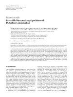
Figure 1: System model.
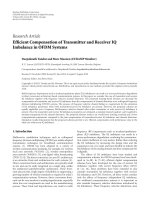
Sensing
Time slot
Sensing
TX TX TX
Sensing
Figure 2: Sensing and transmission phases.
2. Signal Model
Let Y(s) be a one-dimensional random field defined in the
range s
∈ [0, d], with s denoting the spatial variable. As
in [2, 8, 9], we adopt a stationary homogeneous Gaussian
Markov Ornstein-Uhlenbeck (GMOU) model [10]tochar-
acterize the dynamics and spatial correlation of Y (s). GMOU
random fields obey the following linear stochastic differential
equation

dY
(
s
)
= θY
(
s
)
ds + σW
(
s
)
,
(1)
where, by definition, Y(s)
∼ N (0, σ
2
y
)withσ
2
y
= σ/2θ, W(s)
denotes Brownian Motion with unit variance parameter,
and θ, σ are constants reflecting the (spatial) variability
of the field and its noisy behaviour, respectively. According
to this model, the autocorrelation function is given by
R
Y
(s
1

, s
2
) = σ
2
y
e
−θ|s
2
−s
1
|
and, hence, the process is not
(spatially) bandlimited.
The random field is uniformly sampled by N sensor
nodes, with intersensor distance given by d/(N
− 1) 
d/N (see Figure 1). The spatial samples can thus be readily
expressed as follows [11]:
y
k
= Y

k
d
N

=
e
−θ(d/2N)
y

k−1
+ n
k
, k = 1, , N,
(2)
where n
k
∼ N (0, σ
2
y
(1 − e
−θ(d/N)
)).
2.1. Communication Model. As shown in Figure 2,each
time slot is composed of two distinctive phases namely,
the sensing phase and the transmission phase. In the for-
mer, each sensor collects and stores in a local buffer a
large block of n independent and consecutive observations
EURASIP Journal on Wireless Communications and Networking 3
{y
(i)
k
}
n
i
=1
={y
(1)
k
, , y

(n)
k
}. Next, in the transmission
phase,
{y
(i)
k
}
n
i
=1
is block-encoded into a length-n codeword
{u
(i)
k
(v
k
)}
n
i
=1
in codebook C at a rate of R
k
bits per sample.
The encoding (quantization) process is modeled through the
auxiliary random variable u
k
= y
k
+ z

k
with z
k
standing for
memoryless Gaussian noise with variance σ
2
z
k
and statistically
independent of y
k
(for the ease of notation, we drop the
sample index.) . The corresponding codeword index v
k
∈
{
1, ,2
nR
k
}; k = 1 N is then conveyed to the FC, in
atotalofm/N channel uses, over one of the Northogonal
channels (for other encoding schemes, such as Compress-
and-Estimate in Section 3.2, v
k
denotes the index of the bin to
which the codeword belongs to. For further details, see [3]).
The codeword can only be reliably decoded at the FC if the
encoding rate R
k
satisfies

nR
k
≤
m
N
log
2

1+SNRγ
k

[
b/s
]
,
(3)
where SNR stands for the average signal-to-noise ratio
experienced in the sensor-to-FC channels, and γ
1
, ,γ
N
denote the corresponding channel squared gains. In the
sequel, such gains will be modeled as independent and
exponentially-distributed unit-mean random variables (i.e.,
Rayleigh-fading channels) and independent over time slots
(block fading assumption).
From the set of decoded codewords, the FC reconstructs
the random field Y(s)forall s
∈ [0, d]. As a result of the spa-
tial sampling process and the channel bandwidth constraint,

the reconstructed field

Y(s) is subject to some distortion
which, throughout this paper, will be characterized by the
following metric
D
(
s
)
= E





Y(s) − Y(s)



2

; ∀s ∈
[
0, d
]
. (4)
2.2. Distortion Analysis: A General Framework. For the
distortion metric given by (4), the optimal estimator turns
out to be the posterior mean given all the codewords u
=

[u
1
, ,u
N
]
T
; that is, the MMSE estimator [12, Chapter 10]

Y
(
s
)
= E
[
Y
(
s
)
| u
]
; ∀s ∈
[
0, d
]
.
(5)
For mathematical tractability, however, only the two closest
decoded codewords, namely u
k−1
and u

k
, will be used to
reconstruct Y(s)forall the corresponding intermediate
spatial points (in noiseless scenarios, that is, σ
2
z
k
= 0for
all k, this approach turns out to be optimal due to the
Markovian property of GMOU processes. For the general
case, yet suboptimal, it capitalizes on the codewords which
retain more information on the random field at the spatial
point s) (see Figure 1), that is

Y
(
s
)
= E
[
Y
(
s
)
| u
k−1
, u
k
]
,

∀s ∈

(
k
− 1
)
d
N
, k
d
N

.
(6)
For the ease of notation and without loss of generality, in the
sequel, we assume k
= 1 and, hence, the interval between
observations reads s
∈ [0, d/N]. From [12, Chapter 10], the
distortion associated to the estimator (6)isgivenby
D
k
(
s
)
= σ
2
Y(s)
|u
k−1

,u
k
= σ
2
Y(s)
|u
k−1
−
Cov
2
(
Y
(
s
)
, u
k
| u
k−1
)
σ
2
u
k
|u
k−1
.
(7)
For our signal model and after some algebra, the various
terms in the expression above can be computed as

σ
2
Y(s)
|u
k−1
=

1
σ
2
y
+
e
−θs
(
1
− e
−θs
)
σ
2
y
+ σ
2
z
k−1

−1
,
Cov

(
Y
(
s
)
, u
k
| u
k−1
)
= E
[
(
Y
(
s
)
− E
[
Y
(
s
)
| u
k−1
]
| u
k−1
)
×

(
u
k
− E
[
u
k
| u
k−1
]
| u
k−1
)
]
=

e
−θ(d/N−s)
σ
2
Y(s)
|u
k−1
,
σ
2
u
k
|u
k−1

= e
−θ(d/N−s)
σ
2
Y(s)
|u
k−1
+

1 − e
−θ(d/N−s)

σ
2
y
+ σ
2
z
k
.
(8)
It is worth noting that the variance of the quantization noise
σ
2
z
k−1
and σ
2
z
k

are determined by the encoding strategy in use
at the sensor nodes.
3. Delay-Constrained WSNs
In delay-constrained (DC) networks, the n samples collected
in the sensing phase of a given timeslot must be necessarily
encoded and transmitted to the FC in the corresponding
transmission phase. Bearing this in mind, we particular-
ize the analysis of Section 2.2 and compute the average
distortion for the cases of Delay-Constrained Quantize-
and-Estimate (QEDC) and Compress-and-Estimate (CEDC)
encoding strategies.
3.1. Quantize-and-Estimate: Average Distortion. Here, each
sensor encodes its observation regardless of any side infor-
mation that could be made available to the FC. From [13],
the following inequality holds for the rate at the output of
the kth encoder (quantizer)
R
k
≥ I

y
k
; u
k

b/sample

,
(9)
with I(

·; ·) standing for the mutual information. As dis-
cussed before, the encoding (quantization) process is mod-
eled through the auxiliary variable u
k
= y
k
+ z
k
with z
k
∼
N (0, σ
2
z
k
) and statistically independent of y
k
(see, e.g., [3, 14]
for further details). The minimum rate per sample can be
expressed as follows:
I

y
k
; u
k

=
H
(

u
k
)
− H

u
k
| y
k

=
log

1+
σ
2
y
σ
2
z
k


b/sample

.
(10)
From (3), (9), and (10) we have that, necessarily,
m
N

log
2

1+SNR · γ
k

≥
n log
2

1+
σ
2
y
σ
2
z
k

.
(11)
4 EURASIP Journal on Wireless Communications and Networking
By taking equality in (11), the variance of the quantization
noise yields
σ
2
z
k
=
σ

2
y

1+SNRγ
k

W/N
− 1
, k
= 1, , N,
(12)
with W
= m/n standing for the sample-to-channel uses
ratio. By replacing (12) into (7), the distortion in an arbitrary
spatial point s in the kth segment reads
D
QEDC
k
(
s
)
=
⎛
⎝
1
σ
2
Y
(
s

)
|u
k−1
+
e
−θ(d/N−s)


1+SNRγ
k
(
i
)

W/N
−1



1+SNRγ
k
(
i
)

W/N
−1

(
1

−e
−θ(d/N−s)
)
σ
2
y
+σ
2
y
⎞
⎠
−1
,
(13)
with
σ
2
Y(s)
|u
k−1
=
⎛
⎝
1
σ
2
y
+
e
−θs



1+SNRγ
k
(
i
)

W/N
− 1



1+SNRγ
k
(
i
)

W/N
− 1

(
1
− e
−θs
)
σ
2
y

+ σ
2
y
⎞
⎠
−1
.
(14)
The average distortion (over the spatial variable s) in the kth
network segment can be computed as
D
QEDC
k
=
N
d

d/N
0
D
QEDC
k
(
s
)
ds,
(15)
and, from this, the average distortion (over channel realiza-
tions) follows:
D

QEDC
= E
γ
1
, ,γ
N
⎡
⎣
1
N − 1
N−1

k=1
D
QEDC
k+1
⎤
⎦
. (16)
3.2. Compress-and-Estimate: Average D istortion. In Com-
press-and-Estimate encoding, the FC incorporates some side
information into the decoding process. This extent can be
exploited by the sensors in order to encode their observations
more efficiently. For simplicity, we assume that only the
codeword sent by the adjacent sensor, u
k−1
will be used
as side information for decoding codeword u
k
(alternatively,

we could use all the sensor observations but due to the
spatial Markov property of the random field model, this is
not expected to substantially decrease the encoding rate).
Accordingly, the minimum rate per sample can be expressed
as follows:
R
k
≥ I

y
k
; u
k
| u
k−1

=
H
(
u
k
| u
k−1
)
− H

u
k
| y
k

, u
k−1

=
H

y
k
+ z
k
| u
k−1

− H

y
k
+ z
k
| y
k

=
log
2
⎛
⎝
1+
σ
2

y
k
|u
k−1
σ
2
z
k
⎞
⎠

b/sample

,
(17)
where the second equality is due to the fact that, again, u
k
↔
y
k
↔ u
k−1
form a Markov chain. Clearly, the codeword can
be reliably transmitted if and only if
m
N
log
2

1+SNR · γ

k

≥
n log
2
⎛
⎝
1+
σ
2
y
k
|u
k−1
σ
2
z
k
⎞
⎠
. (18)
By taking equality in (18), the minimum variance of the
quantization noise σ
2
z
k
follows:
σ
2
z

k
=
σ
2
y
k
|u
k−1

1+SNRγ
k

W/N
− 1
, k
= 1, , N,
(19)
where σ
2
y
k
|u
k−1
can be easily computed as:
σ
2
y
k
|u
k−1

= e
−θ(d/N−s)
σ
2
Y(s)
|u
k
+

1 − e
−θ(d/N−s)

σ
2
y
. (20)
From (7), the distortion at an arbitrary spatial point s reads:
D
CEDC
k
(
s
)
=
σ
2
y
σ
2
Y(s)

|u
k−1

e
θ(d/N−s)
− 1

σ
2
y
(
e
θ(d/N−s)
− 1
)
+ σ
2
Y(s)
|u
k−1
+
σ
4
Y(s)
|u
k−1

1+SNRγ
k


−W/N
σ
2
y
(
e
θ(d/N−s)
− 1
)
+ σ
2
Y(s)
|u
k−1
.
(21)
with
σ
2
Y(s)
|u
k−1
=
⎛
⎝
1
σ
2
y
+

e
−θs


1+SNRγ
k
(
i
)

W/N
− 1



1+SNRγ
k
(
i
)

W/N
− 1

(
1
− e
−θs
)
σ

2
y
+σ
2
y
k−1
|u
k−2
⎞
⎠
−1
.
(22)
The average distortion for each network segment can be
computed as follows:
D
CEDC
k
=
N
d

d/N
0
D
CEDC
k
(
s
)

(23)
and, finally, the average distortion (over the channel realiza-
tions and network segments) yields:
D
CEDC
= E
γ
1
, ,γ
N
⎡
⎣
1
N − 1
N−1

k=1
D
CEDC
k+1
⎤
⎦
. (24)
4. Delay-Tolerant WSNs with
Quantize-and-Estimate Encoding
Here, we impose a long-term delay constraint: the Ln samples
collected in L consecutive timeslots must be conveyed to the
FC in such L timeslots. In other words, sensors have now
the flexibility to encode and transmit a variable number of
samples in each time slot (according to channel conditions)

and, by doing so, attain a lower distortion.
EURASIP Journal on Wireless Communications and Networking 5
Let n
k
(i) = α
k
(i)n be the number of samples encoded
in m/N channel uses by sensor k in time-slot i. As in the
previous section, we have that
m
N
log
2

1+SNR · γ
k
(
i
)

≥
α
k
(
i
)
nlog
2

1+

σ
2
y
σ
2
z
k

;
k
= 1, , N.
(25)
By replacing σ
2
z
k
from (25) into (7), the distortion per
timeslot yields
D
QEDT
k,α
k
(i)
(
s
)
=
⎛
⎝
1

σ
2
Y(s)
|u
k−1
+
e
−θ(d/N−s)


1+SNRγ
k
(
i
)

W/N α
k
(i)
−1



1+SNRγ
k
(
i
)

W/N α

k
(i)
−1

(
1
−e
−θ(d/N−s)
)
σ
2
y
+σ
2
y
⎞
⎠
−1
.
(26)
In order to minimize the average distortion over the L
timeslots at an arbitrary spatial point s, we need to solve the
following optimization problem, implicitly, we are assuming
that sensor (k
−1)th encodes at a constant rate over timeslots.
This extent will be verified later on in this section:
min
α
k
(

1
)
, ,α
k
(
L
)
1
L
L

i=1
α
k
(
i
)
D
QEDT
k,α
k
(
i
)
(
s
)
,
s.t.
L


i=1
α
k
(
i
)
n
= Ln,
(27)
where the constraint in (27) is introduced to ensure the
stability of the system. Unfortunately, a closed-form solution
for α
k
(1), , α
k
(L) cannot be obtained for this problem.
Instead, we attempt to solve an approximate problem in
which we assume that only codeword u
k
will be used
by the FC to reconstruct the random field Y(s)ins
∈
[(k − 1)(d/N), k(d/N)]. Yet, suboptimal (the FC will actually
use both codewords, namely u
k
and u
k−1
), this solution
outperforms those obtained in delay-constrained scenarios

(see computer simulations section). Bearing all this in mind,
the new cost function which follows from (26) can be readily
expressed as
ˇ
D
QEDT
k,α
k
(
i
)
(
s
)
= σ
2
Y
(
s
)
|u
k
= σ
2
y

1 − e
−θs

+ σ

2
y
e
−θs

1+SNRγ
k
(
i
)

−W/N α
k
(i)
.
(28)
Clearly, only the second term in the summation of the cost
function
ˇ
D
QEDT
k,α
k
(i)
(s) is relevant to the optimization problem,
which can be rewritten as
min
α
k
(

1
)
, ,α
k
(
L
)
1
L
L

i=1
α
k
(
i
)

1+SNRγ
k
(
i
)

−W/N α
k
(i)
s.t.
1
L

L

i=1
α
k
(
i
)
= 1.
(29)
It is straightforward to show that this problem is convex.
Hence, one can construct the lagrangian as follows:
L
(
λ, α
k
(
1
)
, ,α
k
(
L
))
=
1
L
L

i=1

α
k
(
i
)

1+SNRγ
k
(
i
)

−W/N α
k
(i)
+ λ
⎛
⎝
1
L
L

i=1
α
k
(
i
)
− 1
⎞

⎠
,
(30)
where λ is the Lagrange multiplier. By setting the first
derivative of (30) w.r.t. α
k
(i)tozeroweobtain
α
∗
k
(
i
)
=
W
N
ln

1+SNRγ
k
(
i
)

1 − ω
−1
(
λ
∗
/e

)
,
(31)
with ω
−1
(·) denoting the negative real branch of the Lambert
function [15]. As for the computation of λ
∗
, the future
channel gains (γ
k
(i +1), , γ
k
(L)) would be needed, in
principle. However, as L
→∞this noncasuality requirement
vanishes: by the law of large numbers, we have that
lim
L →∞
1
L
L

i=1
α
∗
k
(
i
)

=
W
N
E
γ

ln

1+SNRγ

1 − ω
−1
(
λ/e
)
(32)
and, hence, λ
∗
can be readily obtained by replacing this last
expression into the constraint of (29), namely
λ
∗
=−σ
2
y

W
N
R ln
(

2
)
+1

e
−(W/N )R ln(2)
(33)
where we have defined
R  E
γ

log
2

1+SNRγ


. (34)
Finally, replacing λ
∗
into (31) yields
α
∗
k
(
i
)
=
log
2


1+SNRγ
k
(
i
)

R
; i
= 1, , L, k = 1, , N,
(35)
and, by using α
∗
k
(i) into (40), the quantization noise for the
kth sensor node reads:
σ
2
z
= σ
2
z
k
=
σ
2
y
2
(W/N )R
− 1

; i
= 1, , L, k = 1, , N.
(36)
which evidences that the encoding rate is constant over
timeslots (as initially assumed) and over sensors too.
4.1. Average Distortion in the Reconstructed Random Field. By
inserting α
∗
k
(i) into the original cost function of (26), the
distortion for an arbitrary point in the kth network segment
reads
D
QEDT
k,α
k
(
i
)
(
s
)
= D
QEDT
k
(
s
)
=
⎛

⎝
1
σ
2
Y
(
s
)
|u
k−1
+
e
−θ(d/N−s)

2
(m/n)R
−1


2
(m/n)R
−1

(
1
−e
−θ(d/N−s)
)
σ
2

y
+σ
2
y
⎞
⎠
−1
.
(37)
6 EURASIP Journal on Wireless Communications and Networking
Interestingly, distortion is not a function of the channel
gain experienced by the kth sensor in timeslot i (i.e.,
distortion does not depend on α
∗
k
(i)). As a result and unlike
in QEDC encoding, the distortion experienced in every
timeslot i
= 1, , L is identical. This can be useful in
applications where a constant distortion level is needed.
After some tedious manipulations, the average distortion
in the entire reconstructedrandomfieldcanbeexpressedas
D
QEDT
=
1
N − 1
N−1

k=1

N
d

d/N
0
D
QEDT
k+1
(
s
)
ds
=


σ
2
y
+ σ
2
z

2
e
θd/N
+ σ
4
y

θd/N



σ
2
y
+ σ
2
z

2
e
θd/N
− σ
4
y

θd/N
−
2σ
4
y

σ
2
y
+ σ
2
z

e

θd/N
− 1



σ
2
y
+ σ
2
z

2
e
θd/N
− σ
4
y

θd/N
(38)
4.2. Buffer Stability Considerations. In order to derive a
closed-form solution of the optimal number of samples to be
encoded in each time slot (α
∗
k
(i)), in (32) we let the number
of timeslots L grow to infinity. Clearly, this might lead to a
situation were buffer occupancy grows without bound, that
is, to buffer unstability. To avoid that, we will encode and

transmit a (slightly) higher number of samples per timeslot,
namely
α

k
(
i
)
n
=
log
2

1+SNRγ
k
(
i
)

R − δ
n>α
∗
k
(
i
)
n,
(39)
with 0 <δ<
R. By doing so, one can prove (see the

appendix) that buffers are stable. Unsurprisingly, this come
at the expense of an increased distortion in the estimates (see
computer simulation results in Section 7).
5. Delay-Tolerant WSNs with
Compress-and-Estimate Encoding
As in previous section, we let n
k
(i) = α
k
(i)n be the number
of samples encoded in m/N channel uses (i.e., one timeslot).
Again, the rate at the output of the C&E encoder must satisfy
m
N
log
2

1+SNR · γ
k
(
i
)

≥ α
k
(
i
)
n log
2

⎛
⎝
1+
σ
2
y
k
|u
k−1
σ
2
z
k
⎞
⎠
.
(40)
To stress that expression (40)differs from (25) in that the
C&E encoder assumes that the FC will use u
k−1
to decode u
k
and, hence, σ
2
y
k
has been replaced by σ
2
y
k

|u
k−1
. Therefore, from
(7) and the definition of σ
2
y
k
|u
k−1
in (20), we have that for the
current block of α
k
(i)n samples the distortion reads
D
CEDT
k,α
k
(i)
(
s
)
=
σ
2
y
σ
2
Y(s)
|u
k−1


e
θ(d/N−s)
− 1

σ
2
y
(
e
θ(d/N−s)
− 1
)
+ σ
2
Y(s)
|u
k−1
+
σ
4
Y(s)
|u
k−1

1+SNRγ
k
)
(
i

)

−m/α
k
(i)n
σ
2
y
(
e
θ(d/N−s)
− 1
)
+ σ
2
Y(s)
|u
k−1
.
(41)
By averaging over L timeslots, the following optimization
problem results:
min
α
k
(
1
)
, ,α
k

(
L
)
1
L
L

i=1
α
k
(
i
)
D
CEDT
k,α
k
(
i
)
(
s
)
, (42)
s.t.
L

i=1
α
k

(
i
)
n
= Ln. (43)
Solving this problem leads to a closed-form solution that is
identical to that of the QEDT case, namely,
α
∗
k
(
i
)
=
log
2

1+SNRγ
k
(
i
)

R
.
(44)
Finally, replacing α
∗
k
(i) into (40) yields

σ
2
z
k
=
σ
2
y
k
|u
k−1
2
(W/N )R
− 1
; i
= 1, , L, k = 1, , N, (45)
that is, the encoding rate in CEDT networks is constant over
sensors and timeslots, as implicitly assumed in the score
function (43). To remark, the stability analysis of Section 4.2
also applies here.
5.1. Average Distortion in the Reconstructed Random Field. By
inserting α
∗
k
(i) into the original cost function of (43), the
distortion for an arbitrary point in the kth segment reads
D
CEDT
k,α
k

(i)
(
s
)
=
σ
2
y
σ
2
Y(s)
|u
k−1

e
θ(d/N−s)
− 1

σ
2
y
(
e
θ(d/N−s)
− 1
)
+ σ
2
Y(s)
|u

k−1
+
σ
4
Y(s)
|u
k−1
2
−(W/N )R
σ
2
y
(
e
θ(d/N−s)
− 1
)
+ σ
2
Y(s)
|u
k−1
.
(46)
As in the QEDT case, distortion is not a function of the
channel gain experienced by the kth sensor in timeslot i.
Hence, the distortion experienced in every timeslot i
=
1, ,L is identical. Therefore, the average distortion for
EURASIP Journal on Wireless Communications and Networking 7

each network segment can be computed in a closed form as
follows:
D
CEDT
k
=
N
d

d/N
0
D
CEDT
k
(
s
)
=

σ
2
y
+ σ
2
z
k−1

σ
2
y

+ σ
2
z
k

e
θd/N
+ σ
4
y

θd/N

σ
2
y
+ σ
2
z
k−1

σ
2
y
+ σ
2
z
k

e

θd/N
− σ
4
y

θd/N
−
σ
4
y

2σ
2
y
+ σ
2
z
k−1
+ σ
2
z
k

e
θd/N
− 1


σ
2

y
+ σ
2
z
k−1

σ
2
y
+ σ
2
z
k

e
θd/N
− σ
4
y

θd/N
.
(47)
Finally, the average distortion in the whole reconstructed
random field yields
D
CEDT
=
1
N − 1

N−1

k=1
D
CEDT
k+1
.
(48)
6. Latency Analysis
In delay-tolerant networks, each sensor encodes and trans-
mits a variable number of samples per timeslot. As a result,
the time elapsed until the FC receives the first n samples
from all the N sensors in the network (which allows for the
reconstruction of the first n realizations of the random field)
is unavoidably larger than in delay-constrained networks. In
this section, we attempt to characterize such latency. To that
aim, we start by analyzing the time needed for one sensor to
transmit n consecutive samples of the random field. Next,
we derive the latency of the QEDT and CEDT encoding
strategies, respectively.
6.1. Latency Analysis for a Single Sensor Node. Let n
∗
k
(i) =

α
∗
k
(i)n be the number of samples encoded in m/N channel
uses in timeslot i. The probability that l

= 0, , n−1samples
are encoded in arbitrary timeslot i can be expressed as
p
l
= Pr

n
∗
k
(
i
)
= l

(49)
= Pr

l
n
≤ α
∗
k
(
i
)
<
l +1
n

; l = 0, ,n − 1. (50)

Besides, we define
p
n
= Pr

n
∗
k
(
i
)
≥ n

(51)
= Pr

α
∗
k
(
i
)
≥ 1

. (52)
On that basis, we model our system as an absorbing Markov
chain [16, Chapter 8] with n transient states (S
1
, ,S
n−1

)
and one absorbing state (S
n
) defined as follows (see,
Figure 3):
S
l
=
⎧
⎪
⎪
⎪
⎪
⎪
⎪
⎪
⎪
⎪
⎪
⎪
⎪
⎪
⎨
⎪
⎪
⎪
⎪
⎪
⎪
⎪

⎪
⎪
⎪
⎪
⎪
⎪
⎩
l samples have beentransmitted
in previous timeslots,
l
= 0, , n − 1,
n ormore sampleshavebeen transmitted
in previous timeslots,
l
= n.
(53)
The transition matrix P of an absorbing Markov chain has
the following canonical form:
P
=

Qr
0
T
1

, (54)
where Q denotes the (n +1)
× (n + 1) transient matrix and r
is a (n +1)

× 1 nonzero vector (otherwise the absorbing state
could never be reached from the transient states). The entries
of the matrix Q can be computed as follows:
q
l, j
=
⎧
⎨
⎩
0 j<l,
p
j−l
otherwise.
(55)
The entries of the (n +1)
× 1 r vector, which denote the
probability of absorbtion from each transient states, are given
by
r
l
= 1 −
n−1

j=0
q
l, j
; l = 0, , n − 1.
(56)
Our goal is to characterize the time elapsed until the
absorbing state is reached or, in other words, the time needed

to transmit n consecutive samples of the local observation
of the random field at sensor k (i.e., sensor latency). For
an absorbing Markov chain, the time to absorbtion, τ,isa
random variable which obeys the so-called Discrete Phase-
type (DPH) distribution. From [17], the probability mass
and cumulative distribution functions can be expressed as:
f
τ
(
t
)
= Pr
(
τ = t
)
= π
T
Q
t−1
r; t = 1, , ∞
(57)
F
τ
(
t
)
= Pr
(
τ ≤ t
)

= 1 − π
T
Q
t
1; t = 1, , ∞
(58)
where the (n +1)
× 1vectorπ is used to define the initial
conditions. Since we assume that initally no samples have
been transmitted, this yields
π
T
=
[
1, 0, ,0
]
T
.
(59)
From all the above, the average time to absorbtion reads:
E
[
τ
]
=
∞

t=1
tf
τ

(
t
)
.
(60)
Alternatively, from [16,Chapter8],onecancompute
u
=
(
I
− Q
1
)
−1
1
(61)
8 EURASIP Journal on Wireless Communications and Networking
q
1,2
= p
1
q
0,1
= p
1
S
0
S
1
S

n−1
S
n
1
q
n−1,n−1
= p
0
q
1,1
= p
0
q
0,0
= p
0
r
n−1
r
0
Transient states Absorbing state
···
.
.
.
.
.
.
.
.

.
.
.
.
Figure 3: An absorbing Markov chain.
the elements of which account the average time to absorbtion
from state S
0
S
n
. Consequently, the average sensor latency
is given by its first element, namely,
E[τ] = u(1).
Finally, we need to derive a closed-form expression for
the set of probabilities
{p
0
, p
1
, , p
n
} defined in (50)and
(52). From (35), we have that
α
∗
k
(
i
)
=

log
2

1+SNRγ
k
(
i
)

R
.
(62)
with
R = E
γ
[log
2
(1 + γSNR)] and, hence,
p
l
= Pr

l
n
≤ α
∗
k
(
i
)

<
l +1
n

=
Pr

l
n
R ≤ log
2

1+SNRγ
k
(
i
)

<
l +1
n
R

=
F
γ

2
((l+1)/n)R
− 1

SNR

−
F
γ

2
(l/n)R
− 1
SNR

(63)
for l
= 0, , n − 1andp
n
= 1 − F
γ
((2
R
− 1)/SNR). For
Rayleigh-fading channels, the CDF of the channel gain is
given by F
γ
(x) = 1 − e
−x
.
6.2. Latency Analysis for QEDT Encoding. At this point, the
interest lies in characterizing the time elapsed until the N
sensors in the network encode and transmit their first n
samples of the random field. Let Ψ be a random variable

which accounts for QEDT latency, namely
Ψ
= max
k=1, ,N
τ
k
,
(64)
where τ
k
stands for the latency associated to the individual
sensor k as defined in the previous section. Since, on the
one hand, sensors experience i.i.d fading channels and, on
the other, codewords from different sensors are decoded
independently, then τ
1
, ,τ
N
turn out to be i.i.d. DPH
random variables with marginal pmf’s and CDFs given by
(57)and(58), respectively. From all the above, the CDF of
the latency associated to QEDT encoding reads
F
Ψ
(
t
)
= Pr
(
Ψ ≤ t

)
= Pr

max
k
τ
k
≤ t

=
Pr
(
τ
1
≤ t, τ
2
≤ t, , τ
N
≤ t
)
= F
N
τ
(
t
)
=

1 − π
T

Q
t
1

N
, t = 1, , ∞.
(65)
The probability mass function can be computed as
f
Ψ
(
t
)
= Pr
(
Ψ = t
)
= F
Ψ
(
t
)
− F
Ψ
(
t
− 1
)
=


1 − π
T
Q
t
1

N
−

1 − π
T
Q
t−1
1

N
, t = 1, , ∞.
(66)
and, from this last expression, the average latency yields
E
[
Ψ
]
=
∞

t=1
tf
Ψ
(

t
)
.
(67)
Intuitively, latency is a monotonically increasing function in
the number of sensors (the more sensors, the larger the time
needed to collect all samples). This extent will be verified in
Section 7 (Simulation and numerical results).
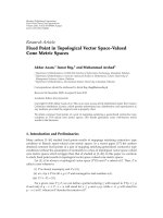
6.3. Latency Analysis for CEDT Encoding. The latency anal-
ysis for CEDT strategies if far more involved due to the
successive encoding of data that C&E schemes entail. In
general, this does not allow for the derivation of closed-form
expressions and, thus, we will resort to an approximate (yet
accurate) model.
In order for the FC to successfully decode the codeword
received from sensor k, the codeword sent by the adjacent
sensor k
− 1 must have been decoded first. Consequently, the
codeword sent by the Nth sensor will be the last one to be
decoded. Since sensors experience i.i.d. fading channels (and,
thus, the number of observations received from different
EURASIP Journal on Wireless Communications and Networking 9
(N − 1)c
0
n
u
1
1
Time
N − 2 N − 1 N

Sensors
Decoded
samples
n
2c
0
n
c
0
n
u
N−2
u
N−1
u
N
Figure 4: Approximate CEDT decoding for latency analysis.
sensors are not time-aligned), when the first n samples sent
by sensor N are ready to be decoded, a total of n + c
o
n>
n samples from sensor N
− 1 have already been decoded
on average. Accordingly, a total of n +(N
− 1)c
o
n samples
from sensor #1 have already been decoded too (see Figure 4).
Hence, the first n realizations of the entire random field can
be reconstructed if, equivalently, n +(N

− 1)c
o
n samples sent
by the first sensor have already been decoded by the FC. The
encoding/decoding process for the first sensor is identical in
C&E and Q&E schemes and, hence, in order to compute the
latency for the reconstruction of the random field,itsuffices
to compute the time to absorbtion for an individual sensor
(sensor #1) as we did in Section 6.1. The only change with
respect to the model given in (54) is that the Markov chain
has now a total of n +(N
− 1)c
o
n states (instead of n) and,
hence, the size and elements of matrix Q and vectors π and r
in (57)and(58) must be adjusted accordingly.
As for parameter c
o
, which exclusively depends on the pdf
of the sensor-to-FC channel gains, it can only be determined
empirically (see next section).
7. Simulations and Numerical Results
Figure 5 depicts the (pertimeslot) distortion in the recon-
structed random field for both the QEDC and QEDT
encoding strategies and different SNR values. For the QEDC
strategy, we show the average value along with the
±σ
confidence interval (to recall that, unlike in the QEDT
case, the distortion in QEDC encoding varies from timeslot
to timeslot). Several conclusions can be drawn. First, for

each curve there exists an optimal operating point; that
is, a network size for which distortion can be minimized.
The intuition behind this fact is that, despite that spatial
variations of the random field are better captured by a denser
grid of sensors, for a total bandwidth constraint the available
rate per sensor progressively diminishes, this resulting into
a more rough quantization of the observations. Thus, the
optimal trade-off between these two effects needs to be
identified. Second, the distortion associated to delay-tolerant
strategies is, as expected, lower than for delay-constrained
ones. Moreover, the lower the average SNR in the sensor-to-
FC channels (namely, sensors with lower transmit power),
2.2dB
SNR
= 10 dB
3dB
SNR
= 0dB
−16
−14
−12
−10
−8
−6
−4
−2
Distortion (dB)
20 40 60 80 100 120 140 160
N
QEDT (δ

= 0)
QEDT (δ
= 0.1)
QEDC
Figure 5: Average distortion versus network size N (W = 150, θd =
10).
δ = 0.1
δ
= 0.05
δ
= 0
0
2
4
6
8
10
12
14
16
18
Average buffer content in blocks of n samples
0 100 200 300 400 500 600 700 800
Time slot
QEDT
Figure 6: Average buffer occupancy versus time (SNR = 0dB).
the higher the gain (up to 3 dB for SNR = 0 dB). Third,
guaranteing buffer stability in the QEDT scheme only results
into a marginal penalty in distortion, as shown in the curves
labeled with δ

= 0andδ = 0.1. Complementarily, in
Figure 6, we depict buffer occupancy for several values of
δ.Forδ
= 0, the system is clearly unstable. Conversely, by
letting δ take positive values, for example, for δ
= 0.1as
in Figure 5, the average buffer occupancy can be kept under
control (with a relatively small average buffer occupancy of
3n samples, in this case). Clearly, increasing δ has a two-
fold effect: the average buffer occupancy diminishes but,
simultaneously, the resulting distortion increases.
The rate at which distortion decreases for the QEDC
and QEDT schemes (evaluated at their respective optimal
10 EURASIP Journal on Wireless Communications and Networking
Δ
SNR
= 4dB
−18
−17
−16
−15
−14
−13
−12
−11
−10
−9
−8
Distortion (dB)
0 5 10 15 20

SNR (dB)
QEDC
QEDT (δ
= 0.1)
QEDT (δ
= 0)
Figure 7: Average distortion versus SNR (W = 150, θd = 10).
2dB
SNR
= 10 dB
3dB
SNR
= 0dB
−18
−16
−14
−12
−10
−8
−6
−4
−2
Distortion (dB)
0 50 100 150 200 250
N
CEDC
CEDT (δ
= 0.1)
CEDT (δ
= 0)

Figure 8: QEDT encoding: average distortion versus network size
(W
= 150, θd = 10).
operating points) for an increasing SNR is shown in Figure 7.
For intermediate distortion values, the gap is approximately
4 dB. That is, for a prescribed distortion level, the energy
consumption in delay-constrained networks is 2.5 times
higher.
Figure 8 illustrates the average distortion in the recon-
structed random field for the CEDC and CEDT encod-
ing strategies. As in quantize-and-estimate encoding, there
exists an optimal number of sensors nodes. Finding such
N
∗
reveals particularly useful for random fields with low
SNR per sensor, since the curve is sharper in this case.
The gap between the minimum distortion attainable by
the CEDC and CEDT schemes (which results from an
−35
−30
−25
−20
−15
−10
Distortion (dB)
0 5 10 15 20
SNR (dB)
QEDT (θ
d
= 10)

CEDT (θ
d
= 10)
QEDT (θ
d
= 1)
CEDT (θ
d
= 1)
Figure 9: Distortion versus SNR (W = 150).
1
1.5
2
2.5
3
3.5
4
4.5
Latency
0 20 40 60 80 100
N
SNR
= 0dB
SNR
= 10 dB
SNR
= 20 dB
Theoretical
Simulations
Figure 10: CEDT encoding: average latency versus network size.

adequate exploitation of channel fluctuation in the delay-
tolerant approach) is approximately 2-3 dB. Concerning
buffer occupancy-distortion tradeoffs, the same comments as
in the quantize-and-estimate case apply.
Next, in Figure 9, we compare the distortion attained
by QEDT/CEDT encoding strategies for random fields with
low and high spatial variabilities (θd
= 1, θd = 10, resp.).
Due to the fact that CEDT is capable of exploiting spatial
correlation, it always outperforms QEDT. Moreover, the
higher the spatial correlation (θd
= 1), the larger the gap
between the curves.
Finally, in Figures 10 and 11 we depict the average
latency for the QEDT and CEDT strategies, respectively.
EURASIP Journal on Wireless Communications and Networking 11
0
5
10
15
20
25
30
35
Latency
51015202530
N
c
0
= 1

c
0
= 0.6
c
0
= 0.3
Approximated theoretical model
Simulated
Figure 11: Average latency versus network size.
Interestingly, there exists a trade-off in terms of attainable
distortion versus latency. Whereas in CEDT encoding latency
exhibits a linear increase in the number of sensors, in QEDT
encoding latency grows logarithmically (i.e., more slowly).
However, CEDT schemes attain a lower distortion than
QEDT ones. Besides, in Figure 10 it is also worth noting
the perfect match between simulations and numerical results
and, unsurprisingly, that the higher the average SNR, the
lower the latency. Also, Figure 11 reveals that by using an
appropriate value of c
o
(i.e., c
o
= 0.6), the latency associated
to the approximate model described in Section 6.3 matches
the actual one.
8. Conclusions
In this paper, we have extensively analyzed the problem of
random field estimation with wireless sensor networks. In
order to characterize the dynamics and spatial correlation
of the random field, we have adopted a stationary homo-

geneous Gaussian Markov Ornstein-Uhlenbeck model. We
have considered two scenarios of interest: delay-constrained
(DC) and delay-tolerant (DT) networks. For each scenario,
we have analyzed two encoding schemes, namely, quantize-
and-estimate (QE) and compress-and-estimate (CE). In all
cases (QEDC, QEDT, CEDC and CEDT), we have carried out
an extensive analysis of the average distortion experienced in
the reconstructed random field. Moreover, for the QEDT and
CEDT strategies we have derived closed-form expressions
of (i) the average distortion in the estimates, and (ii) the
optimal number of samples of the random field to be
encoded in each timeslot (under some simplifying assump-
tions). Interestingly, the resulting pertimeslot distortion in
DT scenarios is deterministic and constant whereas, in DC
scenarios, it ultimately depends on the fading conditions
experienced in each timeslot. Next, we have focused on the
latency associated to the QEDT and CEDT strategies. We
have modeled our system as an absorbing Markov chain and,
on that basis, we have fully characterized the pdf, CDF, and
the average latency for the QEDT case. For CEDT encoding,
we have identified an approximate system model suitable for
the computation of the average latency. Simulation results
reveal that, under a total bandwidth constraint, there exists
an optimal number of sensors for which the distortion in
the reconstructed random field can be minimized (QEDC,
QEDT, CEDC and CEDT cases). This constitutes the best
trade-off in terms of, on the one hand, the ability to
capture the spatial variations of the random field and, on
the other, the persensor channel bandwidth available to
encode observations. Besides, the distortion associated to

delay-tolerant strategies is, as expected, lower than for delay-
constrained ones: some 2-3 dB for both the QE and CE
encoding schemes. Moreover, buffer occupancy can be kept
at very moderate levels (3 timeslots) with a marginal penalty
in terms of distortion (less than 0.3 dB). We also observe that
CE schemes effectively exploit the spatial correlation and, by
doing so, attain a lower distortion than their QE counterparts
(DC and DT scenarios). As far as latency is concerned, we
have empirically shown that CEDT exhibits a linear increase
in the number of sensors whereas in QEDT encoding latency
grows logarithmically (i.e., more slowly). However, CEDT
schemes attain a lower distortion than QEDT ones. Besides,
for the QEDT case, there is a perfect match between simu-
lations and the theoretical model and, for the CEDT case,
latency can be accurately represented by adequately parame-
terizing the aforementioned approximate system model.
Appendix
Buffer Stability Analysis
We want to prove that buffers are stable (i.e., their occupancy
is bounded) for large L.Letb
k
(i) denote the number of
samples in the buffer of the kth sensor in time slot i,with
initial conditions given by b
k
(0) = L
0
n.AfterL timeslots, the
increase in the number of samples stored in the buffer can be
expressed as

b
k
(
L
)
− b
k
(
0
)
= Ln −
L

i=1
α

k
(
i
)
n,
(A.1)
where Ln accounts for the number of samples generated in
those L timeslots, and

L
i
=1
α


k
(i)n with
α

k
(
i
)
=
log
2

1+SNRγ
k
(
i
)

R − δ
>α
∗
k
(
i
)
,
(A.2)
stands for the actual number of samples encoded and
transmitted by the kth sensor node. The probability of
experiencing an increase greater than

n in the number of
samples stored reads
Pr
(
b
k
(
L
)
− b
k
(
0
)
≥ n
)
= Pr
⎛
⎝
Ln −
L

i=1
α

k
(
i
)
n

≥ n
⎞
⎠
=
Pr
⎛
⎝
L

i=1
α

k
(
i
)
≤ L − 
⎞
⎠
.
(A.3)
12 EURASIP Journal on Wireless Communications and Networking
for any
 > 0. Replacing (A.2) into this last expression yields:
Pr
(
b
k
(
L

)
− b
k
(
0
)
≥ n
)
= Pr
⎛
⎝
L

i=1
log
2

1+SNRγ
k
(
i
)

R − δ
≤ L − 
⎞
⎠
=
Pr
⎛

⎝
L

i=1
log
2

1+SNRγ
k
(
i
)

−
LR ≤
(
 − L
)
δ − R
⎞
⎠
=
Pr
⎛
⎝
L

i=1
log
2


1+SNRγ
k
(
i
)

− R

L Var
(
R
)
≤
(
 − L
)
δ − R

L Var
(
R
)
⎞
⎠
,
(A.4)
where we have defined
Var
(

R
)

E
γ


log
2

1+SNRγ(i)

−
R

2

. (A.5)
For large L, we can resort to the central limit theorem by
which
Z
=
L

i=1
log
2

1+SNRγ
k

(
i
)

−
R

L Var
(
R
)
∼ N
(
0, 1
)
.
(A.6)
Hence, as long as δ takes strictly positive values (δ>0), we
have that
lim
L →∞
Pr
(
b
k
(
L
)
− b
k

(
0
)
≥ n
)
= lim
L →∞
Pr

Z ≤
(
 − L
)
δ − R

L Var
(
R
)

=
0.
(A.7)
This result states that, as long as we encode a slightly
higher number of samples per timeslot (which depends on
parameter δ) the probability that the increase in buffer
occupancy exceeds
n samples (for a finite value of )canbe
made arbitrary small for large L. That is, buffers are stable.
Conversely, δ

= 0 yields
lim
L →∞
Pr
(
b
k
(
L
)
− b
k
(
0
)
≥ n
)
δ=0
=
1
2
,
(A.8)
this meaning that, even for arbitrarily large values of
, the
probability that buffer occupancy increases beyond
 n is
unavoidably 1/2 (i.e., unstable buffers).
In addition to this main result, the probability for buffers
to drain after L timeslots can be expressed as

p
drain
= Pr
(
b
k
(
L
)
= 0
)
= Pr
⎛
⎝
L

i=1
α

k
(
i
)
n
≥
(
L + L
0
)
n

⎞
⎠
=
Pr
⎛
⎝
L

i=1
log
2

1+SNRγ
k
(
i
)

R − δ
≥ L + L
0
⎞
⎠
.
(A.9)
By resorting again to the central limit theorem, we have that
for any positive value of δ
lim
L →∞
p

drain
= lim
L →∞
Pr

Z ≥
L
0
R −
(
L + L
0
)
δ

L Var
(
R
)

=
1, (A.10)
and, thus, buffers will drain with probability one after a
sufficiently large number of timeslots.
Acknowledgment
This work is partly supported by the Catalan Government
(2009 SGR 1046), the EC-funded project NEWCOM++
(216715), and the Spanish Ministry of Science and Innova-
tion (FPU grant AP2007-01654).
References

[1] I. F. Akyildiz, W. Su, Y. Sankarasubramaniam, and E. Cayirci,
“Wireless sensor networks: a survey,” Computer Networks, vol.
38, no. 4, pp. 393–422, 2002.
[2] M. C. Vuran and I. F. Akyildiz, “Spatial correlation-based col-
laborative medium access control in wireless sensor networks,”
IEEE/ACM Transactions on Networking, vol. 14, no. 2, pp. 316–
329, 2006.
[3] S. C. Draper and G. W. Wornell, “Side information aware
coding strategies for sensor networks,” IEEE Journal on
Selected Areas in Communications, vol. 22, no. 6, pp. 966–976,
2004.
[4] A. D. Wyner and J. Ziv, “The rate-distortion function for
source coding with side information at the decoder,” IEEE
Transactions on Information Theory, vol. 22, no. 1, pp. 1–10,
1976.
[5] P. Ishwar, A. Kumar, and K. Ramchandran, “Distributed
sampling for dense sensor networks: a bit-conservation prin-
ciple,” in Proceedings of the 2nd International Workshop on
Information Processing in Sensor Networks, vol. 2634 of Lecture
Notes in Computer Science, pp. 17–31, April 2003.
[6] D. Dardari, A. Conti, C. Buratti, and R. Verdone, “Mathe-
matical evaluation of environmental monitoring estimation
error through energy-efficient wireless sensor networks,” IEEE
Transactions on Mobile Computing, vol. 6, no. 7, pp. 790–802,
2007.
[7] A. Dogand
ˇ
zi
´
c and K. Qiu, “Decentralized random-field

estimation for sensor networks using quantized spatially
correlateddata and fusion-center feedback,” IEEE Transactions
on Signal Processing, vol. 56, no. 12, pp. 6069–6085, 2008.
[8] M. Dong, L. Tong, and B. M. Sadler, “Impact of data retrieval
pattern on homogeneous signal field reconstruction in dense
sensor networks,” IEEE Transactions on Signal Processing, vol.
54, no. 11, pp. 4352–4364, 2006.
[9] D. Marco and D. L. Neuhoff, “Reliability vs. efficiency in
distributed source coding for field-gathering sensor net-
works,” in Proceedings of the 3rd International Symposium on
Information Processing in Sensor Networks (IPSN ’04), pp. 161–
168, Berkeley, Calif, USA, April 2004.
[10] I. Karatzas and S. E. Shreve, Brownian Motion and Stochastic
Calculus, Springer, 1988.
[11] S. Finch, “Ornstein-uhlenbeck process,” May 2004,
/>[12] S. M. Kay, Fundamentals of Statistical Signal Processing: Estima-
tion Theory, Prentice-Hall Signal Processing Series, Prentice-
Hall, Englewood Cliffs, NJ, USA, 1993.
[13] T. M. Cover and J. A. Thomas, Elements of Information Theory,
Wiley Series in Telecommunications, Wiley, New York, NY,
USA, 1993.
[14] P. Ishwar, R. Puri, K. Ramchandran, and S. S. Pradhan, “On
rate-constrained distributed estimation in unreliable sensor
networks,” IEEE Journal on Selected Areas in Communications,
vol. 23, no. 4, pp. 765–775, 2005.
EURASIP Journal on Wireless Communications and Networking 13
[15] R. M. Corless, G. H. Gonnet, D. E. G. Hare, D. J. Jeffrey,
andD.E.Knuth,“OntheLambertW function,” Advances in
Computational Mathematics, vol. 5, no. 4, pp. 329–359, 1996.
[16] C. D. Mayer, Matrix Analysis and Applied Linear Algebra,

SIAM, 2001.
[17] M. F. Neuts, Matrix-Geometric Solutions in Stochastic Models:
An Algorithmic Approach, Chapter 2: Probability Distri bution-
sof Phase Type, Dover, 1981.