báo cáo hóa học:" Research Article Channel Characteristics and Performance of MIMO E-SDM Systems in an Indoor Time-Varying Fading Environment" pptx

Hindawi Publishing Corporation
EURASIP Journal on Wireless Communications and Networking
Volume 2010, Article ID 736962, 14 pages
doi:10.1155/2010/736962

Research Article
Channel Characteristics and Performance of MIMO E-SDM
Systems in an Indoor Time-Varying Fading Environment
Huu Phu Bui,1 Hiroshi Nishimoto,2 Yasutaka Ogawa,3 Toshihiko Nishimura,3
and Takeo Ohgane3
1 Faculty

of Electronics & Telecommunications, Hochiminh City University of Natural Sciences, 227 Nguyen Van Cu st.,
Dist. 5, Hochiminh City, Vietnam
2 Information Technology R&D Center, Mitsubishi Electric Corporation, 5-1-1 Ofuna, Kamakura 247-8501, Japan
3 Graduate School of Information Science and Technology, Hokkaido University, Kita 14, Nishi 9, Kita-ku, Sapporo 060-0814, Japan
Correspondence should be addressed to Toshihiko Nishimura,
Received 13 October 2009; Revised 22 January 2010; Accepted 13 March 2010
Academic Editor: Claude Oestges
Copyright © 2010 Huu Phu Bui et al. This is an open access article distributed under the Creative Commons Attribution License,
which permits unrestricted use, distribution, and reproduction in any medium, provided the original work is properly cited.
Multiple-input multiple-output (MIMO) systems employ advanced signal processing techniques. However, the performance is
affected by propagation environments and antenna characteristics. The main contributions of the paper are to investigate Doppler
spectrum based on measured data in a typical meeting room and to evaluate the performance of MIMO systems based on an
eigenbeam-space division multiplexing (E-SDM) technique in an indoor time-varying fading environment, which has various
distributions of scatterers, line-of-sight wave existence, and mutual coupling effect among antennas. We confirm that due to the
mutual coupling among antennas, patterns of antenna elements are changed and different from an omnidirectional one of a
single antenna. Results based on the measured channel data in our measurement campaigns show that received power, channel
autocorrelation, and Doppler spectrum are dependent not only on the direction of terminal motion but also on the antenna
configuration. Even in the obstructed-line-of-sight environment, observed Doppler spectrum is quite different from the theoretical
U-shaped Jakes one. In addition, it has been also shown that a channel change during the time interval between the transmit weight

matrix determination and the actual data transmission can degrade the performance of MIMO E-SDM systems.

1. Introduction
The use of multiple antennas at both ends of a communication link, commonly referred to as a multiple-input multipleoutput (MIMO) system, has been widely studied and is
considered as one of the prospective technologies to provide
high data rate transmission and good performance for
the dramatically growing wireless communications demands
nowadays. Many studies have confirmed that, without
additional power and spectrum compared with conventional single-input single-output (SISO) systems, channel
capacity of MIMO systems can increase in proportion to
the number of antennas in Rayleigh fading environments
[1–3]. Moreover, when channel state information (CSI) is
available at a transmitter (TX), the performance of the
MIMO system can be improved further by applying an
eigenbeam-space division multiplexing (E-SDM) technique,

which is also called eigenmode transmission or singular
value decomposition- (SVD-) based technique [1–6]. In the
E-SDM technique, orthogonal transmit beams are formed
based on the eigenvectors obtained from singular value
decomposition of a MIMO channel matrix, and transmit
data resources can be allocated adaptively. In the ideal case,
in which the transmit weight matrix completely matches an
instantaneous MIMO channel response, spatially orthogonal
substreams with the optimal resource allocation can be
achieved. As a result, a simple maximum ratio combining
(MRC) detector or a spatial filter such as a minimum mean
square error (MMSE) filter or zero-forcing (ZF) filter can
detect the substreams without inter-substream interference,
and the maximum channel capacity is obtained.

In realistic environments, however, due to dynamic
nature of the channel and processing delay at both the TX
and the receiver (RX), a channel transition may cause a


2

EURASIP Journal on Wireless Communications and Networking

severe loss of subchannel orthogonality, which results in
large inter-substream interference. In addition, the channel
change prevents optimal resource allocation from being
achieved. Consequently, based on computer-generated channels assuming the Jakes model [7], we have confirmed that
the performance of MIMO E-SDM systems is degraded
in time-varying fading environments with rich scatterers
[8, 9]. The Jakes model is very simple because required
parameters are very few, and it is easy as regards simulations.
However, actual MIMO systems may be used in line-of-sight
(LOS) environments, and even in a non-LOS (NLOS) case,
scatterers may not be uniformly distributed around an RX
and/or a TX. The geometry-based stochastic channel model
(GSCM) has been proposed for multiple antenna systems
[10–13]. The model includes also the LOS component
and is more comprehensive than the Jakes model. It is
expected that GSCM can explain phenomena in real-life
fading environments. In order to apply GSCM, however,
we need to determine several parameters, and we need
three-dimensional ray tracing or extensive measurement
campaigns [12, 13]. This is much more difficult to apply than
the Jakes model. On the other hand, when using multiple

antennas at both the TX and the RX, mutual coupling
among antenna elements cannot be ignored because it affects
the system performance in practical implementation [14–
16]. Therefore, investigations into the systems in actual
communications are necessary.
MIMO measurement campaigns have already been
extensively conducted as reported in papers such as [6, 15–
18]. However, most of MIMO measurement campaigns have
not explicitly considered the effect of time-varying fading on
the performance of MIMO systems. In [19], measurements
were carried out in a case where a mobile station was moving.
The objective of the study was not to examine the effect of
time-varying channels but to introduce a stochastic MIMO
radio channel model. In [20], the performance of closedloop MIMO (i.e., MIMO E-SDM) systems was investigated
in the fading environment where both TX and RX were fixed,
and scatterers were moving during the experiment. It is said
that the effects of moving scatterers in the environment were
relatively unimportant.
In time-varying wireless communications, Doppler spectrum is a useful measure to evaluate the mobility of
terminals [21]. Then, the Doppler spectrum may affect
the performance of MIMO E-SDM systems in dynamic
channels. Due to various distributions of scatterers, LOS
wave existence, and mutual coupling effect among antennas,
the Doppler spectrum of SISO and MIMO channels in
actual environments are, in general, different from the
theoretical analyses. To the best of our knowledge, such
work has rarely been considered [22, 23]. In [22], Doppler
spectrum of a SISO channel was investigated where the
base and user were both stationary, but scatterers in the
environment were moving, causing time variations in the

channel response. In [23], Doppler spectrum of a 8 × 8
MIMO channel was examined in both indoor and outdoor
environments. The results in [22, 23] revealed that the effects
of moving scatterers in the environment were relatively
unimportant. Both of [22, 23] did not consider the Doppler

spectrum in the case of the LOS condition and the effect
of the spectrum on the performance of MIMO systems.
Also, array configurations have been considered based on
measurement campaigns to clarify the channel capacity [24,
25]. The studies did not consider the effect of the array
configuration to the MIMO E-SDM performance in timevarying environments.
We conducted SISO and MIMO measurement campaigns at a 5.2 GHz frequency band in an indoor timevarying fading environment. In our measurement campaigns, the RX was moved while the TX and scatterers
were fixed. We evaluated the MIMO system performance
partially using the HIPERLAN/2 standard [26]. Based on
the measured channel data, in this paper, we examined
some channel properties such as antenna pattern, received
power, channel autocorrelation, and Doppler spectrum of
both SISO and MIMO cases. Then, we evaluated the biterror rate (BER) performance of MIMO E-SDM systems in
the environment.
The main contributions of the paper are the following.
(i) The radiation patterns of the antenna elements in
MIMO case are examined. It can be seen that the
patterns change from the SISO case due to mutual
coupling. This has an effect on the received power.
(ii) The received power, channel autocorrelation,
and Doppler spectrum in actual fading LOS
and obstructed LOS (OLOS) environments are
considered. The results show that they are dependent
on the direction of the RX motion, the antenna array

configuration, and the propagation environments.
(iii) The performance of the E-SDM system is investigated
in actual time-varying fading environments. It is
shown that the performance can be degraded by the
channel change during the time interval between the
transmit weight matrix determination and the actual
data transmission.
The paper is organized as follows. In the next section, a
detailed measurement setup for our experiment is presented.
In Section 3, the antenna pattern of a two-element array is
considered. Based on the measured channel data, we examine
received power in Section 4 and channel autocorrelation and
Doppler spectrum in Section 5 for both SISO and MIMO
cases. To investigate the performance of MIMO E-SDM
systems in actual environments, we first describe the systems
in Section 6. Then, a procedure of applying measured data
for evaluation of the system performance in an indoor timevarying fading environment is given in Section 7. Based
on the measured data, the performance of MIMO E-SDM
systems in the environment is evaluated in Section 8. The
conclusions are provided in Section 9.

2. Channel Measurement Setup
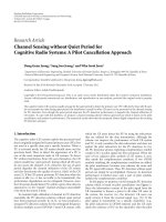
The measurement campaigns were carried out in a meeting
room in a building of the Graduate School of Information
Science and Technology, Hokkaido University, as shown in
Figure 1. The room has an area of about 95 m2 . The walls of


EURASIP Journal on Wireless Communications and Networking

3

Windows

Walls: plasterboard

Console
Ceilling height = 2.6 m
4m

TX

Pillar

RX

3.5 m

8.3 m
Partition

y
12 m
x
y
499th
measurement point

0.5λ

Motion
0.5λ
TX-x
TX-y
TX antennas

RX-x
RX-y

0th
measurement point
RX antennas

Reinforced concrete
Metal

Figure 1: Measurement site (top view).

the room consist of plasterboard around reinforced concrete
pillars and metal doors. The metal whiteboard behind the
TX was fixed on the wall, and the bottom of the whiteboard
was 1 m above the floor, whereas the TX and RX were placed
0.9 m above the floor. In the room, TX and RX antennas,
omnidirectional colinear antennas AT-CL010 (TSS JAPAN),
were placed on two tables separated by 4 m. The nominal
gain of these antennas on the horizontal plane was about
4 dBi.
On the RX side, a stepping motor was used to move the
RX array along the x- or y-axis during the experiments. Each
step of the motor was 0.0088 cm. This motor was exactly

controlled by a personal computer. The RX array was stopped
at every 10 steps (equal to 0.088 cm) of the motor. Channels
were measured at intervals of 0.088 cm, and we had a total
of 500 spatial measurement points. Therefore, the length of
the measurement route was 500 × 0.088 cm = 44 cm. Here,
we chose the length of 44 cm because it covered several
wavelengths of signal and the difference of pathloss measured
at the first point and the last point was less than 1 dB.
Channels were measured for all the TX and the RX
antenna pairs through a vector network analyzer (VNA), as
shown in Figure 2. RF switches at both the TX and the RX
sides were controlled by a personal computer and selected
a TX antenna and an RX antenna, respectively. Measured
data were then saved in the computer. The unselected antennas were automatically connected to 50 Ω dummy loads.

TX

RX

RF switch
50 Ω

RF switch
50 Ω

Transmission port

50 Ω

VNA

50 Ω

Reception port

Measured data
RF switch controller

PC

RF switch controller

Figure 2: Channel measurement system.

The measurement band was from 5.15 GHz to 5.40 GHz
(bandwidth = 250 MHz), and we obtained 1601 frequency
domain data with 156.25 kHz interval. Each channel was
averaged over 10 snapshots in order to reduce thermal noise
included in the raw measurements. We examined both SISO
and real 2 × 2 MIMO systems. For the MIMO case, the
antenna spacing was 3 and 6 cm (half- and one wavelength
at 5 GHz), and two array orientations (TX-x/RX-x (endfire)


4

EURASIP Journal on Wireless Communications and Networking
TX

RX

y

#1 #2

that the measurement campaigns were conducted while no
one was in the room, to ensure statistical stationarity of
propagation.

x

y

3. Antenna Patterns

#1 #2

x

(a) TX-x/RX-x
TX

RX
y

#2
#1

#2

y

#1
x

x

(b) TX-y/RX-y

Figure 3: Antenna array orientations.

RX antennas

(a) OLOS environment (TX antennas are behind the partition)

TX antennas

RX antennas

1m
0.9 m

(b) LOS environment

Figure 4: Measurement environments.

and TX-y/RX-y (broadside)) along the x- and the y-axes,
respectively, were examined, as shown in Figure 3. When
there was a metal partition between the TX and RX antennas,
we had an OLOS environment, as shown in Figure 4(a). In
the absence of the partition, we had a LOS environment, as

shown in Figure 4(b).
The total of channel response matrix data was 1601 ×
500 = 800 500 obtained for each case of the direction of
the RX antenna motion, the array orientation, the antenna
spacing, and the LOS/OLOS condition. It should be noted

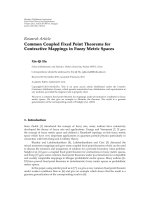
It is well known that when antenna spacing (AS) among
elements is not large enough, there exists mutual coupling
among the elements and their patterns are changed. In
MIMO systems, due to the limitation of space, especially
at mobile stations, the antenna spacing may be small. As
a result, mutual coupling among antennas may be large,
and this would affect the system performance. Thus, in this
section, we consider the antenna pattern for a two-element
linear array.
The patterns for the two-element array with AS of 0.5λ
and 1.0λ used in our measurement campaigns are shown
in Figure 5 (solid curves). The dashed curve corresponding
to the pattern of a single antenna is also included for
comparison. The patterns were obtained by conducting 360◦
measurement of the antennas in an anechoic chamber. It is
seen that the single antenna has an almost omnidirectional
pattern because it does not have the mutual coupling effect.
However, in the multiple antenna case, the patterns are
very different from an omnidirectional one. The antenna
gain seems to decrease as the AS becomes smaller. On the
other hand, the patterns tend to become similar to the
omnidirectional one as the AS becomes larger. The numbers
under each pattern correspond to the ones in Figure 3.
Given the TX-x/RX-x orientation, the RX end is located

in the 0◦ direction with respect to the TX end, and the TX
end is located in the 180◦ direction with respect to the RX
end. Thus, the direct wave departs from the TX end in the 0◦
direction and arrives at the RX end in the 180◦ direction. On
the other hand, given the TX-y/RX-y orientation, the RX end
is located in the 90◦ direction with respect to the TX end, and
the TX end is also located in the 90◦ direction with respect to
the RX end. Thus, the direct wave departs from the TX end
and arrives at the RX end in the 90◦ direction. The gains at
the 0◦ and 180◦ directions tend to be smaller than those at
the 90◦ direction, especially in the case of AS = 0.5λ. These
phenomena are shown in Figure 6.

4. Received Power
In this section, based on the measured channel data, we
examine received power of both SISO and MIMO channels.
Received power of the SISO channel in the frequency
domain at the first spatial measurement position is shown
in Figure 7. It should be noted that the first spatial measurement position when the RX array moves along the x-axis is
different from the one when the array moves along the yaxis, as shown in Figure 8. It is seen from Figure 7 that the
received power for the LOS condition is generally larger than
the power for the OLOS condition due to the direct wave.
Received power of the SISO channel in the spatial domain
at the frequency of 5.15 GHz is shown in Figure 9. It can be
seen that the power fluctuation is much dependent on the


EURASIP Journal on Wireless Communications and Networking
90◦

90◦

180◦

90◦

0◦ 180◦

−90◦
6 3 0 −3 (dBi)

5

0◦

−90◦
6 3 0 −3 (dBi)

#1

90◦

180◦

0◦ 180◦

−90◦
6 3 0 −3 (dBi)

#2

(a) AS = 0.5 λ

0◦

−90◦
6 3 0 −3 (dBi)

#1

#2

(b) AS = 1.0 λ

Figure 5: Antenna patterns for a two-element array with mutual coupling (solid curves) and single isolated antenna pattern (dashed curve).

90◦

90◦

90◦

90◦

TX-x/RX-x
180◦

0◦

180◦

−90◦

0◦

y

−90◦

6 3 0 −3 (dBi) #1

180◦

−90◦
6 3 0 −3 (dBi) #1

#2

6 3 0 −3 (dBi)

x

O

TX

0◦ 180◦

0◦

−90◦
6 3 0 −3 (dBi) #2

RX

(a) Lower gain for TX-x/RX-x
180◦

0◦

−90◦

90◦

90◦

−90◦

TX-y/RX-y
0◦
#2
6 3 0 −3 (dBi)
180◦

90◦

180◦
6 3 0 −3 (dBi)
0◦

90◦

90◦

y

0◦
#1
6 3 0 −3 (dBi)
TX

#2

x

−90◦

180◦
6 3 0 −3 (dBi)

O

#1

RX

(b) Higher gain for TX-y/RX-y

Figure 6: Antenna gain toward the direct wave for the case of AS = 0.5 λ.

direction of the RX array motion. In the LOS environment,
the power fluctuates more rapidly when the array moves
along the x-axis than when it moves along the y-axis. The
interval of the ripples of the power, when the RX motion is
along the x-axis, is about 3 cm (half-wavelength at 5 GHz).
This can be explained as follows. The most dominant wave
was the direct wave (to +x direction) from the TX to the RX.

It is conjectured that other dominant waves were the reflected
wave (to +x direction) from the wall behind the TX array and
the reflected wave (to −x direction) from the wall behind the
RX array. These three waves caused a standing wave along the
x-axis.
Received power of the SISO channel averaged over the
1601 frequency domain data at each spatial measurement


6

EURASIP Journal on Wireless Communications and Networking

Received power (dB)

−40

1st measurement position when
RX motion along the x-axis

y

−50

Motion

−60

x

−70

Motion

−80
−90

5.15

5.2

5.25
5.3
Frequency (GHz)

5.35

1st measurement position when
RX motion along the y-axis
RX side

5.4

Figure 8: The first spatial measurement position.

LOS
OLOS

−40

(a) RX motion along the x-axis
Received power (dB)

Received power (dB)

−40
−50
−60
−70

5.15

−60
−70
−80
−90

−80
−90

−50

5.2

5.25
5.3
Frequency (GHz)

5.35

0

5.4

10
20
30
Spatial measurement position (cm)

40

LOS
OLOS
(a) RX motion along the x-axis

LOS
OLOS

−40

Figure 7: Received power of SISO channel in the frequency domain
at the first spatial measurement position.

position is shown in Figure 10. It is confirmed that the power
for the LOS condition is higher than that for the OLOS
condition due to the direct wave. It can also be seen that in
the OLOS case, the power is almost the same in both cases of
the RX array motion; meanwhile in the LOS case, the power
when the array motion is along the x-axis is more variable
than when the motion is along the y-axis.
Received power of 2 × 2 MIMO channels averaged over
the four channels and 1601 frequency domain data at each
spatial measurement position is shown in Figure 11. As in
the SISO case, the power for the LOS condition is higher
than that for the OLOS condition due to the direct wave.
Here, we can see that in the LOS case, the power for the TXy/RX-y orientation is considerably larger than that for the
TX-x/RX-x one when the antenna spacing is 0.5λ. However,
the power is almost the same for both of the TX-y/RX-y
orientation and TX-x/RX-x one when the antenna spacing
is 1.0 λ. This is due to the effect of mutual coupling between
antenna elements. When AS = 0.5λ, the antenna gain toward
the direct wave for the TX-y/RX-y orientation is much

Received power (dB)

(b) RX motion along the y-axis
−50
−60
−70
−80
−90

0

10
20
30
Spatial measurement position (cm)

40

LOS
OLOS
(b) RX motion along the y-axis

Figure 9: Received power of SISO channel in the spatial domain at
the frequency of 5.15 GHz.

higher than that for the TX-x/RX-x orientation, as seen from
Figures 5(a) and 6. However, when AS = 1.0λ, the antenna
gain toward the direct wave for the TX-x/RX-x orientation
is almost the same as that for the TX-y/RX-y orientation, as
seen from Figure 5(b).


EURASIP Journal on Wireless Communications and Networking

Received power (dB)

−40

−45

−50

−55

−60

0

10
20
30
Spatial measurement position (cm)

40

RX motion along the x-axis
RX motion along the y-axis

LOS
OLOS

Figure 10: Received power of SISO channel averaged over the
frequency domain data at each spatial measurement position.

5. Channel Autocorrelation and Doppler
Spectrum in the Indoor Fading Environment
In this section, based on our measured channel data, we
examine channel autocorrelation and Doppler spectrum of
both SISO and MIMO cases.

We assume that a mobile terminal is moving at a constant
velocity v. With a time interval Δt, the distance Δl that the
mobile terminal has moved is given by
Δl = vΔt.

(1)

It is well known that the maximum Doppler frequency fD
occurring during the mobile terminal’s motion is as follows:
fD =

v
fc ,
c

(2)

where c is the speed of light (c = 3 × 108 m/s) and fc is the
carrier frequency of the mobile terminal.
Combining (1) and (2), we have
fD =

Δl
,
λΔt

(3)

where λ is the wavelength of the carrier frequency.
Assuming that the time interval between the adjacent

measurement points (Δl = 0.088 cm) is 0.5 milliseconds
(Δt = 0.5 milliseconds), then fD is calculated from (3) as
follows:
fD =

0.088 (cm)
5.7 (cm) × 0.5 (ms)

7

the x- and y-axes are shown in Figure 12. The channel
autocorrelation was estimated by averaging over the spatial
domain data and the 1601 frequency domain data. If we
divide the measurement distance (abscissa) in Figure 12 by
the velocity v, we have the channel autocorrelation versus
time. The Doppler spectra of both the measured data and
the Jakes model were calculated by applying the 450-point
DFT process to the time domain channel autocorrelation
after multiplying it by the Hamming window. It can be seen
that the channel autocorrelation and Doppler spectrum are
much dependent on the direction of the RX motion. The
channel autocorrelation in the LOS environment fluctuates
much more when the RX moves along the x-axis than
when it moves along the y-axis. In the LOS case, the power
spectrum density (PSD) is mainly concentrated around fD
of ±31 Hz when the RX moves along the x-axis. This is
because most of dominant incoming waves were the direct
wave (+x direction) from the TX to the RX, the reflected
wave (+x direction) from the wall behind the TX, and the
reflected wave (−x direction) from the wall behind the RX. It

should be noted that the interval of the ripples of the channel
autocorrelation is about 3 cm (the half wavelength at 5 GHz).
When the RX moves along the y-axis, on the other hand,
the PSD is mainly distributed around the Doppler frequency
of 0 Hz. The reason is that the direction of RX motion
is approximately perpendicular to most of the dominant
incoming waves. In the OLOS case, the PSD was expected
to be the U-shaped Jakes spectrum. However, as seen from
Figure 12, the observed PSD is quite different from the one
in the Jakes model. The reason for this is considered to be
that scatterers in the indoor environment are not uniformly
distributed around an RX as well as those that are assumed
in the Jakes model.
The channel autocorrelation and Doppler spectrum for
fD = 31 Hz of 2 × 2 MIMO channels are shown in Figure 13.
Here, the channel autocorrelation was estimated by averaging
over the four channels as well as the spatial domain and
frequency domain data. The Doppler spectrum, as in the
SISO case, was calculated by applying the 450-point DFT
process to the time domain channel autocorrelation after
multiplying it by the Hamming window. It is observed that
the channel autocorrelation and Doppler spectrum of the
2 × 2 MIMO case are quite similar to those of the SISO
case. In addition, from Figure 13, it can also be observed
that the channel autocorrelation and Doppler spectrum are
dependent not only on the direction of the RX motion but
also on the array orientation and the antenna spacing. This
is due to the effect of the mutual coupling between antenna
elements at both the TX and the RX, as shown in Figure 5.
Even in the OLOS case, the Doppler spectrum of MIMO

channels is different from the U-shaped Jakes one.

(4)

31 Hz,
where the carrier frequency was assumed to be the center of
the measurement band ( fc = 5.275 GHz).
The channel autocorrelation and Doppler spectrum for
fD = 31 Hz of the SISO case when the RX moves along

6. MIMO E-SDM Systems
Before investigating the performance of MIMO E-SDM
systems in actual time-varying fading environments, the
concept of a MIMO E-SDM system is briefly described in the
section. For more details on the system, refer to [4].


8

EURASIP Journal on Wireless Communications and Networking
−40

−40

−50

−55

−60

RX motion along the y-axis
Received power (dB)

Received power (dB)

RX motion along the x-axis
−45

0

10
20
30
Spatial measurement position (cm)
TX-y/RX-y
TX-x/RX-x

−45

−50

−55

−60

40

0

10

20
30
Spatial measurement position (cm)

40

LOS
OLOS
(a) AS = 0.5 λ

−40

−40

−45

−50

−55

−60

RX motion along the y-axis
Received power (dB)

Received power (dB)

RX motion along the x-axis

0

10
20
30
Spatial measurement position (cm)
TX-y/RX-y
TX-x/RX-x

40

−45

−50

−55

−60

0

10
20
30
Spatial measurement position (cm)

40

LOS
OLOS
(b) AS = 1.0 λ

Figure 11: Received power of 2 × 2 MIMO channels averaged over the four channels and frequency domain data at each spatial measurement
position.

A block diagram of a MIMO E-SDM system with Ntx
antennas at a TX and Nrx antennas at an RX is shown
in Figure 14. When MIMO CSI is available at the TX,
orthogonal transmit beams can be formed by eigenvalue
decomposition of the matrix HH H, where H denotes the
Nrx ×Ntx MIMO channel matrix, and (·)H denotes Hermitian
transpose. The E-SDM technique is assumed to be used for
downlink (DL) transmission. This study also assumes that
the channel is narrow enough so that no frequency selective
fading occurs, and that the average power of each substream
prior to power control is identical.
At the TX side, an input stream is divided into K
substreams (K ≤ min(Ntx , Nrx )). Then, signals before
transmission are driven by a TX weight matrix to form
orthogonal eigenbeams and control power allocation. At the
RX side, received signals are detected by an RX weight matrix.
The Ntx × K TX weight matrix W tx is determined as
√

W tx = U P,

(5)

where U is the Ntx × K MIMO channel matrix obtained by
the eigenvalue decomposition as
H H H = UΛU H ,

Λ = diag(λ1 , . . . , λK ).

(6)

Here, λ1 ≥ · · · ≥ λK > 0 are positive eigenvalues of
HH H. The columns of U are the eigenvectors corresponding
to those positive eigenvalues, and P = diag(P1 , . . . , PK ) is
the
√ diagonal transmit power matrix. It should be noted that
P = diag( P1 , . . . , PK ) holds.
In an ideal MIMO E-SDM system, in which the TX
weight matrix completely matches an instantaneous MIMO
channel response, spatially orthogonal substreams with
optimal resource allocation can be achieved. Under the
circumstance, received signals can easily be demultiplexed
by using a maximal ratio combining (MRC) or spatial filtering weight. However, in time-varying fading environments
spatial filtering weight is a better choice to mitigate the
degradation of system performance [5].


EURASIP Journal on Wireless Communications and Networking

9
15

1

10
Power spectral density (dB)

Channel autocorrelation

0.75

0.5

Jakes model

5

0

0.25
−5

Jakes spectrum
−10
−45

0
0

5

10
15
Measurement distance (cm)

20

−30

−15

0
15
Frequency (Hz)

30

45

30

45

LOS
OLOS
(a) RX motion along the x-axis

15

1

10
Power spectral density (dB)

Channel autocorrelation

0.75

0.5

Jakes model

5

0

0.25
−5

Jakes spectrum
0
0

5

10
15
Measurement distance (cm)

20

−10
−45

−30

−15

0
15
Frequency (Hz)

LOS
OLOS
(b) RX motion along the y-axis

Figure 12: Channel autocorrelation and Doppler spectrum for fD = 31 Hz of SISO channel.

The signal-to-noise power ratio of the kth detected
substream is given by
γk =

λk Pk Ps
,
σ2

(7)

where Ps = E[|s1 (t)|2 ] = · · · = E[|sK (t)|2 ], and σ 2 is
noise power. This indicates that the quality of each detected
substream is different. Therefore, the channel capacity and
performance of MIMO E-SDM systems can be improved by
adapting the TX data resource and power allocation [4].


TX-x/RX-x
0.75

0.5
Jakes model

0.25
0

0
5
10 15 20
Measurement distance (cm)

15
10

TX-x/RX-x

5
0
−5 Jakes spectrum
−10
−45 −30 −15 0

Channel autocorrelation

1

1
TX-y/RX-y
0.75
0.5

Jakes model

0.25
0

15 30 45
Frequency (Hz)

Power spectral density (dB)

EURASIP Journal on Wireless Communications and Networking
Power spectral density (dB)

Channel autocorrelation

10

0
5
10 15 20
Measurement distance (cm)

15
TX-y/RX-y

10
5
0
−5

Jakes spectrum

−10
−45 −30 −15 0

15 30 45
Frequency (Hz)

LOS
OLOS

0.75
0.5
Jakes model

0.25
0

0
5
10 15 20
Measurement distance (cm)

15
10

TX-x/RX-x

5

0
−5

Jakes spectrum

−10
−45 −30 −15 0

1
TX-y/RX-y
0.75
0.5
Jakes model
0.25
0

15 30 45
Frequency (Hz)

Power spectral density (dB)

TX-x/RX-x

Channel autocorrelation

1

Power spectral density (dB)

Channel autocorrelation

(a) RX array motion along the x-axis and AS = 0.5 λ

0
5
10 15 20
Measurement distance (cm)

15
TX-y/RX-y

10
5
0
−5

Jakes spectrum

−10
−45 −30 −15 0

15 30 45
Frequency (Hz)

LOS
OLOS

0.75

Jakes model

0.5
0.25
0

0
5
10 15 20
Measurement distance (cm)

15
10

TX-x/RX-x

5
0
−5

Jakes spectrum

−10
−45 −30 −15 0

1
TX-y/RX-y
0.75
Jakes model
0.5
0.25

0

15 30 45
Frequency (Hz)

Power spectral density (dB)

TX-x/RX-x

Channel autocorrelation

1

Power spectral density (dB)

Channel autocorrelation

(b) RX array motion along the y-axis and AS = 0.5 λ

0
5
10 15 20
Measurement distance (cm)

15
TX-y/RX-y

10
5
0

−5

Jakes spectrum

−10
−45 −30 −15 0

15 30 45
Frequency (Hz)

LOS
OLOS

0.75
0.5
Jakes model
0.25
0

0
5
10 15 20
Measurement distance (cm)

15
10

TX-x/RX-x

5

0
−5

Jakes spectrum

−10
−45 −30 −15 0

15 30 45
Frequency (Hz)

1
TX-y/RX-y
0.75
0.5
Jakes model
0.25
0
0
5
10 15 20
Measurement distance (cm)

Power spectral density (dB)

TX-x/RX-x

Channel autocorrelation

1

Power spectral density (dB)

Channel autocorrelation

(c) RX array motion along the x-axis and AS = 1.0 λ
15
TX-y/RX-y

10
5
0
−5

Jakes spectrum

−10
−45 −30 −15 0

15 30 45
Frequency (Hz)

LOS
OLOS
(d) RX array motion along the y-axis and AS = 1.0 λ

Figure 13: Channel autocorrelation and Doppler spectrum for fD = 31 Hz of 2×2 MIMO channels.


EURASIP Journal on Wireless Communications and Networking

x1

s1
s2

Input
MUX

.
.
.

TX
weight
matrix

sK

.
.
.
xNtx

Beam 2
.
.
.

r1

y1

r2

Beam 1

x2

11

y2

.
.
.

RX
weight
matrix

.
.
.

Beam K rNrx

Base station

Output
DEMUX

yK
Terminal

Figure 14: Block diagram of a MIMO E-SDM system.

Tf

ACK

DL ACK
packet

τ

DL ACK
packet

Table 1: Simulation Parameters of MIMO E-SDM System.

DL
packet

Figure 15: TDD transmission frame format.

7. A Procedure of Adapting Measured
Data for Performance Evaluation in
Dynamic Channels
The E-SDM technique is assumed to be used in a time
division duplexing (TDD) system (Although a TDD system is

considered in the paper, the obtained results are equivalently
applied to a frequency division duplex system in which CSI
is estimated at the RX and then fed back to the TX.), such
as HIPERLAN/2 [26]. The TX weights are determined by the
channel responses estimated by the uplink acknowledgment
(ACK) packet periodically transmitted at times i × T f (i =
0, 1, . . .), and DL packet transmission is done at times i ×
T f + τ, as shown in Figure 15. The terminal was assumed to
be moving at the constant velocity v yielding fD = 31 Hz,
as stated in Section 5. Here, we assumed that the frame
duration of the TDD system T f was 2.0 milliseconds, as in
the HIPERLAN/2 standard [26], and the time delay τ for the
actual DL data transmission from ACK was 1.5 milliseconds.
Also, as mentioned earlier, in the experiments, we measured
MIMO channels at 500 spatially different points along the xor the y-axis. If the MIMO channels at measurement points
4k (k = 0, 1, . . .) were those for the uplink ACK packets, then
the MIMO channels at the measurement points 4k + 3 were
those for the DL packets, as shown in Figure 16(a). This is
because the ratio τ/T f was 3/4.
If the terminal’s velocity increased up to 3v, then fD also
rose to 93 Hz. In this case, the MIMO channel responses
for the uplink ACK and DL packets were given by the
measurement points 12k and 12k + 9, respectively, as shown
in Figure 16(b).

8. Performance Analyses of MIMO E-SDM
Systems in the Time-Varying Fading
Enviroment
8.1. Simulation Parameters. As mentioned earlier, we
obtained 800 500 measured MIMO channel matrices in

each case of the array orientation, the direction of the

Items
No. of TX & RX antennas
Resource control
Modulation schemes
Data rate
Data burst length
Training symbols
Frame duration (T f )
Delay from ACK (τ)
Max Doppler frequencies
( fD )
Thermal noise
RX signal processing

Parameters
2×2
Minimum BER criterion
based on Chernoff upper-bound [4]
QPSK, 16QAM
4 bits/symbol
48 symbols (no coding)
15 PN symbols (BPSK)
2.0 milliseconds
1.5 milliseconds
31 & 93 Hz
Additive white Gaussian noise
Zero-forcing weight

RX array motion, the antenna spacing, and the LOS/OLOS
condition. In this section, we used them to evaluate the
BER performance of MIMO E-SDM systems in the indoor
time-varying fading environment. The BER performance
was obtained under simulation parameters shown in Table 1.
All the channel data were regarded as frequency flat fading
channels. The validity of this assumption is as follows.
We assumed the DL packet duration of 0.12 milliseconds. This value is not shown in Table 1 because it does not
explicitly affect the results. Because we have 48 symbols in
the DL packet, the symbol duration is 0.0025 milliseconds.
Then, the bandwidth is 400 kHz when the roll-off parameter
is 0. On the other hand, as examined in [15], the time
delay spread in the measurement site was less than 40 ns;
thus the channel coherence bandwidth was considered to be
wider than 2.5 MHz. The transmission bandwidth is much
narrower than the coherence bandwidth, and we can assume
the frequency flat fading.
The data rate was set to 2 bps/Hz (2 bits per symbol
duration) per TX antenna; therefore, the total data rate was
fixed constantly at 4 bps/Hz (4 bits per symbol duration)
for the 2×2 MIMO system. The number of substreams
was dependent on the resource adaptation, specifically
the modulation scheme and the transmit power. We had
two cases of the resource selection, namely, 16QAM×1 (1
stream) and QPSK×2 (2 streams). The reason why we need
resource selection is because we should send more bits
over a substream with higher SNR and fewer bits over a


12

EURASIP Journal on Wireless Communications and Networking
ACK

ACK

ACK

DL
packet

DL
packet

···

0
Tf

DL
packet

···

3

ACK

4

···

7

8

ACK
DL
packet
···

11 12

τ

ACK

DL
packet
···

15

ACK

···

0

Measurement

points

DL
packet

···

9
Tf

(a) fD = 31 Hz

···

12

DL
packet

···

21

ACK

···

24

···

33 36

τ

DL
packet
···

···

45 Measurement
points

(b) fD = 93 Hz

Figure 16: Uplink and downlink MIMO positions for the different fD .

10−3
10−4
10−5

TX-y/RX-y
AS = 0.5λ

10−2
10−3
10−4

10−1

10−5

10
20
30
40
Normalised total TX power (dB)

100

100
Average BER

10−2

10−1
Average BER

Average BER

10−1

100
TX-x/RX-x
AS = 0.5λ

TX-x/RX-x
AS = 1λ

10−2
10−3
10−4

10−1
Average BER

100

10−5

10
20
30
40
Normalised total TX power (dB)

TX-y/RX-y
AS = 1λ

10−2
10−3
10−4
10−5

10
20
30
40
Normalised total TX power (dB)

10
20
30
40
Normalised total TX power (dB)

LOS
OLOS
Ideal case (τ = 0)
fD = 31 Hz
fD = 93 Hz
(a) RX array motion along the x-axis

100

10−3
10−4
10−5

10−2
10−3
10−4

10−1

TX-x/RX-x
AS = 1λ

10−2

10−3
10−4

10−1

10−5

10−5

10
20
30
40
Normalised total TX power (dB)

100

100
Average BER

10−2

10−1

TX-y/RX-y
AS = 0.5λ

Average BER

10−1

TX-x/RX-x
AS = 0.5λ

Average BER

Average BER

100

10
20
30
40
Normalised total TX power (dB)

10
20
30
40
Normalised total TX power (dB)

TX-y/RX-y
AS = 1λ

10−2
10−3
10−4
10−5
10

20
30
40
Normalised total TX power (dB)

LOS
OLOS
Ideal case (τ = 0)
fD = 31 Hz
fD = 93 Hz
(b) RX array motion along the y-axis

Figure 17: BER performance of 2 × 2 MIMO E-SDM system.

substream with lower SNR to obtain better BER under the
fixed data rate requirement. Thus, we need to determine
the modulation schemes for each substream considering the
SNR that was stated in Section 6. Also, we need to allocate
transmit power to each substream properly. The modulation
and power allocation are determined in such a way that the
upper bound of BER has the lowest value [4].

The HIPERLAN/2 system may be used in some different
scenarios as described in [26], and depending on the
scenarios, the mobility of mobile terminals may be fixed,
walking speed, or slow vehicles limited within 10 m/s. In this
paper, two values of fD of 31 and 93 Hz, which correspond
to two terminal’s velocities of 1.8 and 5.4 m/s for the carrier
frequency of 5.2 GHz, were considered. The mobility can

EURASIP Journal on Wireless Communications and Networking
be considered as walking speed or slow vehicles. For those
terminal velocities, we can assume that both of the uplink
and the downlink packet duration were so short that the
channel change during the duration was negligible.
8.2. Simulation Results. The average BER performance of
2 × 2 MIMO E-SDM system versus normalized total TX
power for fD = 31 and 93 Hz is shown in Figure 17. Many
conventional studies have evaluated the performance of
MIMO systems as a function of average SNR. However, in
NLOS or OLOS environments, the transmit power must
be higher than in LOS environments in order to obtain
the same average SNR. Therefore, for fair comparison, the
performance evaluation of MIMO systems should be done
under the same transmit power condition as in [15]. In this
study, the BER performance of MIMO E-SDM systems in
LOS and OLOS environments was examined as a function
of the normalized total transmit power. The normalized
total TX power is the total TX power that is normalized
by the value yielding Es /N0 = 0 dB when we have only
the direct wave in the SISO-LOS transmission environment.
This value was measured in an anechoic chamber with the
same measurement setup mentioned in Section 2. Here, Es
is received signal energy per symbol and N0 is the noise
power density. The ideal case in Figure 17 is that where the
time delay from ACK to actual DL data transmission is equal
to zero (i.e., τ = 0); that is, the channel for the E-SDM
transmission is exactly the same as the estimated one for the
weight matrix determination and resource allocation.

BER performance in the LOS environment is better than
that in the OLOS one due to the higher received power,
as shown in Figure 11. The BER performance is related to
the direction of the RX motion. Better performance can
be obtained in the LOS environment when the motion is
along the y-axis than when it is along the x-axis. This is due
to the effect of Dopper spectrum. As seen from Figure 13,
the Doppler spectrum is distributed around 0 Hz in the
LOS case for the RX motion along the y-axis, whereas it is
concentrated around ± fD for the RX motion along the xaxis. It can be easily seen that the more distributed around
0 Hz the Doppler spectrum is, the better BER performance is
obtained because of the less channel transition. In addition,
the BER performance is also related to the antenna orientation. Better BER performance is obtained for the TX-y/RX-y
orientation than for the TX-x/RX-x orientation in the case
of the LOS environment and AS = 0.5 λ. This is because the
antenna gain for the opposite end in the MIMO system was
higher for the TX-y/RX-y orientation than for the TX-x/RXx orientation due to the effect of mutual coupling among
antenna elements, as shown in Figure 6. As a result, higher
received power was obtained for the TX-y/RX-y orientation
than for the TX-x/RX-x orientation in both cases of the
RX array motion along the x- and the y-axes in the LOS
environment and AS = 0.5 λ, as shown in Figure 11.
Furthermore, as in simulation results based on computer
generated channels assuming the Jakes model [8, 9], the
higher fD was, the more the BER performance was degraded
in the indoor fading environment. This is because greater
channel change during the time interval τ caused larger

13

inter-substream interference and prevented optimal resource
allocation from being achieved. Therefore, a countermeasure
such as a channel prediction scheme [8, 9] may be necessary
for MIMO E-SDM transmission in fast time-varying fading
environments.

9. Conclusions
In this paper, we have presented an experiment for measuring
SISO and 2 × 2 MIMO channel responses at the 5.2 GHz
frequency band in an indoor time-varying fading environment. In the environment, not only OLOS condition but
also LOS condition was considered; scatterers were located at
both the TX and the RX, and were not necessarily distributed
uniformly; the effect of mutual coupling among antennas
was also taken into account.
We first considered the antenna patterns of SISO and
MIMO systems. Different from the SISO case where the
antenna has an omnidirectional pattern, in the MIMO case,
the patterns of antenna elements are changed due to the
mutual coupling among antennas, and the antenna gain
seems to decrease as the AS becomes smaller.
Based on the measured data, we second examined
received power, channel autocorrelation, and Doppler spectrum. The results showed that these fading properties are
dependent not only on the direction of the RX motion but
also on the array configuration and propagation environments. These are due to the effects of various distributions of
scatterers, multipath signals, LOS wave existence, and mutual
coupling among antenna elements. Unlike theoretical analysis, Doppler spectrum in the indoor fading environment is
different from the U-shaped Jakes one.
Finally, based on the measured data, the performance
of MIMO E-SDM systems was evaluated. Simulation results
showed that a channel change during the time interval

between the transmit weight matrix determination and
the actual data transmission could degrade the system
performance in indoor communications. It was shown that
the performance relates to the Doppler spectrum. Therefore,
a channel prediction scheme may be necessary for the
systems in indoor fast time-varying fading environments.

References
[1] E. Telatar, “Capacity of multi-antenna Gaussian channels,”
European Transactions on Telecommunications, vol. 10, no. 6,
pp. 585–595, 1999.
[2] D. Gesbert, M. Shafi, D.-S. Shiu, P. J. Smith, and A. Naguib,
“From theory to practice: an overview of MIMO space-time
coded wireless systems,” IEEE Journal on Selected Areas in
Communications, vol. 21, no. 3, pp. 281–302, 2003.
[3] A. J. Paulraj, D. A. Gore, R. U. Nabar, and H. Bă lcskei,
o
An overview of MIMO communications—a key to gigabit
wireless,” Proceedings of the IEEE, vol. 92, no. 2, pp. 198–217,
2004.
[4] K. Miyashita, T. Nishimura, T. Ohgane, Y. Ogawa, Y. Takatori,
and K. Cho, “High data-rate transmission with eigenbeamspace division multiplexing (E-SDM) in a MIMO channel,” in
Proceedings of IEEE Vehicular Technology Conference (VTC ’02Fall), vol. 3, pp. 1302–1306, Vancouver, Canada, September
2002.


14

EURASIP Journal on Wireless Communications and Networking

[5] G. Lebrun, J. Gao, and M. Faulkner, “MIMO transmission
over a time-varying channel using SVD,” IEEE Transactions on
Wireless Communications, vol. 4, no. 2, pp. 757–764, 2005.
[6] S. H. Ting, K. Sakaguchi, and K. Araki, “A robust and
low complexity adaptive algorithm for MIMO eigenmode
transmission system with experimental validation,” IEEE
Transactions on Wireless Communications, vol. 5, no. 7, pp.
1775–1784, 2006.
[7] W. C. Jakes, Microwave Mobile Communications, John Wiley &
Sons, New York, NY, USA, 1974.
[8] T. Nishimura, T. Tsutsumi, T. Ohgane, and Y. Ogawa,
“Compensation of channel information error using first order
extrapolation in eigenbeam space division multiplexing (ESDM),” in Proceedings of International Conference on Wireless
Communications and Applied Computational Electromagnetics
(ACES ’05), pp. 44–47, Honolulu, Hawaii, USA, April 2005.
[9] B. H. Phu, Y. Ogawa, T. Ohgane, and T. Nishimura, “Extrapolation of time-varying MIMO channels for an E-SDM system,”
in Proceedings of IEEE Vehicular Technology Conference (VTC
’06-Spring), vol. 4, pp. 1748–1752, Melbourne, Australia, May
2006.
[10] J. Fuhl, A. F. Molisch, and E. Bonek, “Unified channel
model for mobile radio systems with smart antennas,” IEE
Proceedings Radar, Sonar and Navigation, vol. 145, no. 1, pp.
32–41, 1998.
[11] H. Hofstetter and G. Steinbă ck, A geometry based stochastic
o
channel model for MIMO systems,” in Proceedings of Internationa ITG Workshop on Smart Antennas (WSA 04), pp. 194
199, Munich, Germany, March 2004.
ă
[12] E. Bonek, W. Weichselberger, M. Herdin, and H. Ozcelik,
“A geometry-based stochastic MIMO channel model for 4G

indoor broadband packet access,” in Proceedings of 18th
General Assembly of the International Union of Radio Science
(URSI ’05), New Delhi, India, October 2005, C03.1.
[13] J. Karedal, F. Tufvesson, N. Czink, et al., “A geometry-based
stochastic MIMO model for vehicle-to-vehicle communications,” IEEE Transactions on Wireless Communications, vol. 8,
no. 7, pp. 3646–3657, 2009.
[14] J. W. Wallace and M. A. Jensen, “Mutual coupling in MIMO
wireless systems: a rigorous network theory analysis,” IEEE
Transactions on Wireless Communications, vol. 3, no. 4, pp.
1317–1325, 2004.
[15] H. Nishimoto, Y. Ogawa, T. Nishimura, and T. Ohgane,
“Measurement-based performance evaluation of MIMO spatial multiplexing in a multipath-rich indoor environment,”
IEEE Transactions on Antennas and Propagation, vol. 55, no.
12, pp. 3677–3689, 2007.
[16] Y. Ogawa, H. Nishimoto, T. Nishimura, and T. Ohgane,
“Performance of MIMO spatial multiplexing in indoor lineof-sight environments,” in Proceedings of IEEE Vehicular
Technology Conference (VTC ’05-Fall), vol. 4, pp. 23982402,
Dallas, Tex, USA, September 2005.
ă
[17] N. Czink, X. Yin, H. Ozcelik, M. Herdin, E. Bonek, and
B. H. Fleury, “Cluster characteristics in a MIMO indoor
propagation environment,” IEEE Transactions on Wireless
Communications, vol. 6, no. 4, pp. 1465–1474, 2007.
[18] V.-M. Kolmonen, J. Kivinen, L. Vuokko, and P. Vainikainen,
“5.3-GHz MIMO radio channel sounder,” IEEE Transactions
on Instrumentation and Measurement, vol. 55, no. 4, pp. 1263–
1269, 2006.
[19] J. P. Kermoal, L. Schumacher, K. I. Pedersen, P. E. Mogensen,
and F. Frederiksen, “A stochastic MIMO radio channel model
with experimental validation,” IEEE Journal on Selected Areas

in Communications, vol. 20, no. 6, pp. 1211–1226, 2002.

[20] K. Mizutani, K. Sakaguchi, J. Takada, and K. Araki, “Measurement of time-varying MIMO channel for performance
analysis of closed-loop transmission,” in IEEE Vehicular
Technology Conference (VTC ’06-Spring), vol. 6, pp. 2854–
2858, Melbourne, Australia, May 2006.
[21] P. Stoica and R. Moses, Introduction to Spectral Analysis,
Prentice Hall, New York, NY, USA, 1997.
[22] A. Domazetovic, L. J. Greenstein, N. B. Mandayam, and I.
Seskar, “Estimating the Doppler spectrum of a short-range
fixed wireless channel,” IEEE Communications Letters, vol. 7,
no. 5, pp. 227–229, 2003.
[23] J. W. Wallace and M. A. Jensen, “Time-varying MIMO channels: measurement, analysis, and modeling,” IEEE Tranactions
on Antennas and Propagation, vol. 54, no. 11, pp. 3265–3273,
2006.
[24] K. Sulonen, P. Suvikunnas, L. Vuokko, J. Kivinen, and P.
Vainikainen, “Comparison of MIMO antenna configurations
in picocell and microcell environments,” IEEE Journal on
Selected Areas in Communications, vol. 21, no. 5, pp. 703–712,
2003.
[25] K. Nishimori, Y. Makise, M. Ida, R. Kudo, and K. Tsunekawa,
“Channel capacity measurement of 8 x 2 MIMO transmission
by antenna configurations in an actual cellular environment,”
IEEE Transactions on Antennas and Propagation, vol. 54, no.
11, pp. 3285–3291, 2006.
[26] “Broadband Radio Access Networks (BRAN); High Performance Radio Local Area Network (HIPERLAN) Type
2; requirements and architectures for wireless broadband
access,” Tech. Rep. TR 101 031 V2.2.1 (1999-01), European
Telecommunications Standards Institute, Sophia Antipolis,
France, January 1999.