Mobile and Wireless Communications-Physical layer development and implementation 2012 Part 8 docx
Bạn đang xem bản rút gọn của tài liệu. Xem và tải ngay bản đầy đủ của tài liệu tại đây (670.83 KB, 20 trang )
High-Rate,ReliableCommunicationswithHybridSpace-TimeCodes 131
symbols to antennas is shown in Table 2. Using this code, n
S
+ n
B
symbols are transmitted
per channel use, for a code rate equal to
T
BS
n
nn
.
(23)
Fig. 6. ZF-SQRD LQOSTBC Architecture Transmitter/Receiver
ANTENNA
Symbol Period
1 2 3 4
(VBLAST)
S
n
2
1
3
5
1
k
s
s
s
*
2
*
6
*
2
k
s
s
s
1
7
3
k
s
s
s
*
*
8
*
4
k
s
s
s
(ABBA)
T
S
S
n
n
n
2
1
B
nk
k
k
s
s
s
4
2
1
*
14
*
1
*
2
B
nk
k
k
s
s
s
24
4
3
B
nk
k
k
s
s
s
*
34
*
3
*
4
B
nk
k
k
s
s
s
Table 2. ZF-SQRD LQOSTBC Symbol to Antenna Mapping with
S
nk 4
Since the transmitter has no knowledge of the channel, all symbols must be transmitted with
equal energy. In the ABBA layers, each symbol’s transmission is spread across multiple time
intervals; in consequence, the signal constellations must be scaled accordingly. If E
v
is the
average energy of the signal constellation employed by each antenna in the VBLAST layers,
then the average constellation energy E
a
of the ABBA layers is given by E
a
=E
v
/n
a
. It should
be noted that the coding schemes referenced above use a single constellation, resulting in
unequal symbol energy and suboptimal BER performance.
The system equation for ZF-SQRD LQOSTBC over four symbol periods may be written as
follows, where subindices indicate antenna number, and superindices indicate symbol
period within a block:
)4()1(
)4(
1
)1(
1
,2,1,
,12,11,1
)4()1(
)4(
1
)1(
1
RR
TRRR
T
RR
nn
A
abba
nnnn
n
nn
nn
nn
S
S
hhh
hhh
yy
yy
,
(24)
or equivalently,
NHSY
.
(25)
Matrix
4
R
n
CY
represents the symbols received in a block. Matrix H is the channel
matrix defined above. Matrix
4
R
n
CN
represents the noise added to each received
symbol. Matrix S is composed of a spatial multiplexing block and n
B
ABBA blocks. The
spatial multiplexing block S
spa
is defined as:
)4()1(
)4(
1
)1(
1
*
414
*
2434
*
43
*
21
SSSSSS
nnnnnn
spa
ss
ss
ssss
ssss
S
,
(26)
which corresponds to the VBLAST layer mapping in Table 2. The ABBA block is defined as:
abba
n
abbaabba
abba
B
SSSS
21
,
(27)
where every element of equation (27) is given by:
)4()1(
)4(
1
)1(
1
)4(
2
)1(
2
)4(
3
)1(
3
*
12
*
34
*
21
*
43
*
34
*
12
*
43
*
21
ll
ll
ll
ll
kkkk
kkkk
kkkk
kkkk
abba
B
ss
ss
ss
ss
ssss
ssss
ssss
ssss
S
,
(28)
with l = n
S
+ 4B, k = 4(B − 1 + n
S
) and B = 1, 2,…, n
B
. Rewriting the system equation (24) as a
linear dispersion code, we have:
MobileandWirelessCommunications:Physicallayerdevelopmentandimplementation132
*)4(
)3(
*)2(
)1(
*)4(
1
)3(
1
*)2(
1
)1(
1
*)4(
)3(
*)2(
)1(
*)4(
1
)3(
1
*)2(
1
)1(
1
R
R
R
R
R
R
R
R
n
n
n
n
LDabbaspa
n
n
n
n
n
n
n
n
n
n
n
n
SHH
y
y
y
y
y
y
y
y
,
(29)
expressed in compact form as:
LDLDLDLD
NSHY ,
(30)
where H
LD
is a linear dispersion matrix with two blocks, one corresponding to the V-BLAST
layers and another to the ABBA layers. The V-BLAST block H
spa
is given by:
spa
nn
spa
n
spa
n
spa
n
spaspa
spa
SRRR
S
HHH
HHH
H
,2,1,
,12,11,1
,
(31)
where
*
,
,
*
,
,
,
000
000
000
000
ji
ji
ji
ji
spa
ji
h
h
h
h
H
,
(32)
for
R
ni ,,2,1 and
S
nj ,,2,1
. The ABBA block
abba
H
is itself a block matrix; it is
given by:
High-Rate,ReliableCommunicationswithHybridSpace-TimeCodes 133
*)4(
)3(
*)2(
)1(
*)4(
1
)3(
1
*)2(
1
)1(
1
*)4(
)3(
*)2(
)1(
*)4(
1
)3(
1
*)2(
1
)1(
1
R
R
R
R
R
R
R
R
n
n
n
n
LDabbaspa
n
n
n
n
n
n
n
n
n
n
n
n
SHH
y
y
y
y
y
y
y
y
,
(29)
expressed in compact form as:
LDLDLDLD
NSHY
,
(30)
where H
LD
is a linear dispersion matrix with two blocks, one corresponding to the V-BLAST
layers and another to the ABBA layers. The V-BLAST block H
spa
is given by:
spa
nn
spa
n
spa
n
spa
n
spaspa
spa
SRRR
S
HHH
HHH
H
,2,1,
,12,11,1
,
(31)
where
*
,
,
*
,
,
,
000
000
000
000
ji
ji
ji
ji
spa
ji
h
h
h
h
H
,
(32)
for
R
ni ,,2,1 and
S
nj ,,2,1
. The ABBA block
abba
H
is itself a block matrix; it is
given by:
abba
nn
abba
n
abba
n
abba
n
abbaabba
abba
SRRR
S
HHH
HHH
H
,2,1,
,12,11,1
,
(33)
where every element of equation (33) is given by:
*
3,
*
2,
*
1,
*
,
2,3,,1,
*
1,
*
,
*
3,
*
2,
,1,2,3,
,
lililili
lililili
lililili
lililili
abba
ki
hhhh
hhhh
hhhh
hhhh
H
,
(34)
for
R
ni ,,2,1
,
B
nk ,,2,1
and l = n
S
+ 4B. The matrix
spa
ji
H
,
of H
LD
that links the
j
th
spatial antenna with the i
th
receiver antenna. Likewise,
abba
ki
H
,
links the k
th
ABBA block to
the i
th
receiver antenna. To complete the reformulation of system equation (24), it remains to
rearrange matrix S. We define S
LD
as:
T
abba
LD
spa
LDLD
SSS
(35)
where
T
nnnn
spa
LD
SSSS
ssssssssS
)4()3()2()1()4(
1
)3(
1
)2(
1
)1(
1
(36)
and the ABBA block for n
A
= 4 is, then, given by:
T
llllnnnn
abba
LD
ssssssssS
SSSS
)1()1(
1
)1(
2
)1(
3
)1(
4
)1(
3
)1(
2
)1(
1
.
(37)
We have rewritten the hybrid space-time matrices as linear dispersion code matrices. Now
we can substitute the original V-BLAST plus ABBA hybrid transceiver with a simpler,
purely spatial system with N
T
= 4n
S
+n
A
n
B
transmit antennas like is depicted in Figure 7 and
without distinction between the ABBA and VBLAST layers.
5. Receiver Architectures for Hybrid Space-Time Codes
Since schemes ZF-SQRD LSTBC and ZF-SQRD LQOSTBC are equivalent to a purely spatial
system with N
T
transmit antennas, it is possible to propose a linear detector based on the
MobileandWirelessCommunications:Physicallayerdevelopmentandimplementation134
sorted QR decomposition and OSIC, that takes advantage of the structure of the linear
dispersion matrices to achieve low complexity and high performance.
5.1 OSIC Detection for Hybrid Schemes Proposed
We first calculate HC Sorted QR (Hybrid Coding Sorted QR) of the matrix H
LD
=Q
LD
R
LD
where Q
LD
is a unitary matrix and R
LD
is an upper triangular matrix. By multiplying the
received signal equations (10) and (35) by
H
LD
Q
, the modified received vector is:
LDLDLDLD
H
LDLD
NSRYQY
~
~
,
(38)
if vector S
LD
is transmitted. Note that the statistical properties of the noise term
LD
N
~
remain unchanged. Due to the upper triangular structure of R
LD
, the k
th
element of
LD
Y
~
is:
T
N
ki
kiikkkkk
nsrsry
1
,,
~~
.
(39)
Symbols are estimated in sequence, from lower stream to higher stream, using OSIC;
assuming that all previous decisions are correct; the interference can be perfectly cancelled
in each step except for the additive noise. The estimated symbol
k
s
is given by:
kk
N
ki
iikk
k
r
sry
s
T
,
1
,
ˆ
D
,
(40)
where
k
s
ˆ
is the estimate of
k
s
and D[.] is a decision device that maps its argument to the
closest constellation point. Therefore the receiver requires calculating the QR decomposition
for the linear dispersion matrix H
LD
; the main challenge lies in finding the most efficient way
to obtain this decomposition.
We use the permutation vector order provided by HC Sorted QR algorithm to reorder the
received symbols; the QR decomposition is obtained using the modified Gram-Schmidt
(MGS) algorithm.
5.2 HC Sorted QR Decomposition
Matrix H
LD
is
RAT
nnN
for both hybrid schemes. A direct application of MGS on it would
result in unacceptable complexity. However, taking advantage of the structure imposed on
H
LD
by the proposed code, we can decrease this complexity significantly. We now explain
how this simplification is obtained.
From the equations (15) and (30) we can see that the structure presented for the H
LD
matrix
allows us to reduce the computational complexity that is required for to calculate the HC
High-Rate,ReliableCommunicationswithHybridSpace-TimeCodes 135
sorted QR decomposition and OSIC, that takes advantage of the structure of the linear
dispersion matrices to achieve low complexity and high performance.
5.1 OSIC Detection for Hybrid Schemes Proposed
We first calculate HC Sorted QR (Hybrid Coding Sorted QR) of the matrix H
LD
=Q
LD
R
LD
where Q
LD
is a unitary matrix and R
LD
is an upper triangular matrix. By multiplying the
received signal equations (10) and (35) by
H
LD
Q
, the modified received vector is:
LDLDLDLD
H
LDLD
NSRYQY
~
~
,
(38)
if vector S
LD
is transmitted. Note that the statistical properties of the noise term
LD
N
~
remain unchanged. Due to the upper triangular structure of R
LD
, the k
th
element of
LD
Y
~
is:
T
N
ki
kiikkkkk
nsrsry
1
,,
~~
.
(39)
Symbols are estimated in sequence, from lower stream to higher stream, using OSIC;
assuming that all previous decisions are correct; the interference can be perfectly cancelled
in each step except for the additive noise. The estimated symbol
k
s
is given by:
kk
N
ki
iikk
k
r
sry
s
T
,
1
,
ˆ
D
,
(40)
where
k
s
ˆ
is the estimate of
k
s
and D[.] is a decision device that maps its argument to the
closest constellation point. Therefore the receiver requires calculating the QR decomposition
for the linear dispersion matrix H
LD
; the main challenge lies in finding the most efficient way
to obtain this decomposition.
We use the permutation vector order provided by HC Sorted QR algorithm to reorder the
received symbols; the QR decomposition is obtained using the modified Gram-Schmidt
(MGS) algorithm.
5.2 HC Sorted QR Decomposition
Matrix H
LD
is
RAT
nnN
for both hybrid schemes. A direct application of MGS on it would
result in unacceptable complexity. However, taking advantage of the structure imposed on
H
LD
by the proposed code, we can decrease this complexity significantly. We now explain
how this simplification is obtained.
From the equations (15) and (30) we can see that the structure presented for the H
LD
matrix
allows us to reduce the computational complexity that is required for to calculate the HC
Sorted QR decomposition, since many of the elements of each matrix are equal, and their
locations in each matrix are fixed and can be calculated in advance. This method involves
obtaining the QR decomposition of the H
LD
matrix in two stages: first we obtain the QR
decomposition corresponding to the spatial layers of the hybrid system; in the second stage
we calculate the QR decomposition for the diversity layers.
As a first step, we calculate the QR decomposition H = Q
m
R
m
using the Sorted QR algorithm;
in this process, we also produce vector order which specifies the detection order of the
spatial layers. Then, using Q
m
and R
m
, and non normalized columns of the matrix H, we
build the matrices
ala
div
H
or
abba
div
H
. The next step is analogous to MGS: column k + 1 is
normalized and used to fill column k+2 of each block (Alamouti/ABBA); the process is
repeated for the remaining columns for each block of
ala
div
H
or
abba
div
H
. In the process, matrix
R
LD
is also calculated. A block diagram of the process is shown in the Figure 7.
Fig. 7. HC Sorted QR Process Using MGS Algorithm
The structure of matrices Q
LD
and R
LD
, and their relation to Q
m
and R
m
, has been detailed in
(Cortez et al., 2007), (Kim et al., 2006), (Le et al., 2005). The complete process is presented in
two stages. In the first stage the algorithm 1 takes the channel matrix H and outputs the
intermediate matrices Q
m
, R
m
and vector order.
MobileandWirelessCommunications:Physicallayerdevelopmentandimplementation136
Algorithm 1. HC Sorted QR of the Spatial Layers
1: INPUT:
TR
nn
H
,
L
,
nsym
,
S
n
2: OUPUT:
m
Q
,
m
R
, order
3:
HQ
m
,
0
TT
nn
m
R
, ]:1:1[ nsymorden
4: for 1i to
S
n
do
5:
jQk
mnij
S
:,minarg
:
6: Exchange columns i and k of
m
Q
and
m
R
7: Exchange columns
1)1(:1:
LiLi and 1)1(:1:
LkLk of
order
8:
2
)(:,),( iQiiR
mm
9:
),(/)(:,)(:, iiRiQiQ
mmm
10: for
1
ij to
T
n
do
11:
)(:,)(:,),( jQiQjiR
m
H
mm
12:
),()(:,)(:,)(:, jiRiQjQjQ
mmmm
13: endfor
14: endfor
The structure for the matrices Q
m
and R
m
are:
TRSR
SRR
TS
S
T
S
S
nnnn
nnn
nn
n
n
n
n
m
hhqq
hhqq
hhqq
Q
,1,
,1,
,21,2
,21,2
,1
1,1
,11,1
,
(41)
TSSs
TSS
TSS
nnnn
nnn
nnn
m
rr
rrr
rrrr
R
,,
,21,2,2
,11,1,11,1
00
0
.
(42)
We choose the first n
S
columns of Q
m
and the first n
S
rows of R
m
to built the matrices Q
spa
and R
spa
with the next structure:
High-Rate,ReliableCommunicationswithHybridSpace-TimeCodes 137
Algorithm 1. HC Sorted QR of the Spatial Layers
1: INPUT:
TR
nn
H
,
L
,
nsym
,
S
n
2: OUPUT:
m
Q
,
m
R
, order
3:
HQ
m
,
0
TT
nn
m
R
, ]:1:1[ nsymorden
4: for 1i to
S
n
do
5:
jQk
mnij
S
:,minarg
:
6: Exchange columns i and k of
m
Q
and
m
R
7: Exchange columns
1)1(:1:
LiLi and 1)1(:1:
LkLk of
order
8:
2
)(:,),( iQiiR
mm
9:
),(/)(:,)(:, iiRiQiQ
mmm
10: for
1
ij to
T
n
do
11:
)(:,)(:,),( jQiQjiR
m
H
mm
12:
),()(:,)(:,)(:, jiRiQjQjQ
mmmm
13: endfor
14: endfor
The structure for the matrices Q
m
and R
m
are:
TRSR
SRR
TS
S
T
S
S
nnnn
nnn
nn
n
n
n
n
m
hhqq
hhqq
hhqq
Q
,1,
,1,
,21,2
,21,2
,1
1,1
,11,1
,
(41)
TSSs
TSS
TSS
nnnn
nnn
nnn
m
rr
rrr
rrrr
R
,,
,21,2,2
,11,1,11,1
00
0
.
(42)
We choose the first n
S
columns of Q
m
and the first n
S
rows of R
m
to built the matrices Q
spa
and R
spa
with the next structure:
SRRR
S
S
nnnn
n
n
spa
qqq
qqq
qqq
Q
,2,1,
,22,21,2
,12,11,1
,
(43)
TSSs
TSS
TSS
nnnn
nnn
nnn
spa
rr
rrr
rrrr
R
,,
,21,2,2
,11,1,11,1
00
0
.
(44)
The matrices Q
spa
and R
spa
represent the contribution of the spatial layers in both hybrid
schemes. The columns with elements
ji
h
,
in equation (41) are non normalized columns that
we used to build the matrices
ala
div
H
and
abba
div
H
that are required in the second stage of the
QR decomposition for the diversity layers. In the case of ZF-SQRD LDSTBC the matrix
ala
div
H
has the following structure:
*
,
*
,
*
1,
*
2,
*
,1
*
,1
*
1,1
*
2,1
,1
1,1
2,11,1
1
1
TR
TR
SRSR
T
T
SS
T
T
SS
nn
nn
nnnn
n
n
nn
n
n
nn
ala
div
hhhh
hhhh
hhhh
H
.
(45)
For the case of ZF-SQRD LQOSTBC the matrix
abba
div
H
with 4
A
n has the structure:
*
2,
*
,
*
2,
*
4,
*
,1
*
2,1
*
4,1
*
2,1
1,1
3,1
3,11,1
TR
TR
SRSR
T
T
SS
T
T
SS
nn
nn
nnnn
n
n
nn
n
n
nn
abba
div
hhhh
hhhh
hhhh
H
.
(46)
Once the matrix
abbaala
div
H
/
is found, the next step is to apply the Sorted QR decomposition
on it. This calculation may be carried out using Algorithm 2 below; the ordering among
elements of the matrix
abbaala
div
H
/
is by block and not by column. It is only necessary to
MobileandWirelessCommunications:Physicallayerdevelopmentandimplementation138
calculate the odd rows and columns of matrices
div
Q
and
div
R
. It can be seen as
ala
div
H
and
abba
div
H
have the same structure, the matrix
abba
div
H
can be seen as a particular case of
ala
div
H
with two Alamouti coders in each block ABBA. The above consideration allows us to use the
same algorithm to calculate the HC Sorted QR decomposition for both schemes. The matrices
div
Q
and
div
R
generated in this part of the process represent the contribution of diversity
layers in the HC Sorted QR decomposition.
Algorithm 2. HC Sorted QR of the Diversity Layers
1: INPUT:
abbaala
div
H
/
,
L
,
nsym
,
B
n ,
S
n
, order
2: OUPUT:
div
Q
,
div
R
, order
3:
abbaala
div
div
HQ
/
, 0
div
R ,
S
Lnm
4: for
2:1i to
B
n2 do
5:
jQk
div
nij
B
:,minarg
2:2:
6: Exchange columns i and i+1 for k and k+1 of
div
Q
and
div
R
7: Exchange columns 1)1(:1:
LimLim and
1)1(:1:
LkmLkm of order
8:
2
)(:,),( iQiiR
divdiv
9:
),(/)(:,)(:, iiRiQiQ
divdivdiv
10:
),()1,1( iiRiiR
divdiv
11:
*
),:2:2()1,1:2:1( iLnQiLnQ
R
div
R
div
12:
*
),1:2:1()1,:2:2( iLnQiLnQ
R
div
R
div
13: for
1
ij to
B
n2 do
14:
)(:,)(:,),( jQiQjiR
divHdivdiv
15: endfor
16:
*
):2:3,()1:2:2,1(
B
div
B
div
LniiRLniiR
17:
*
)1:2:2,():2:3,1(
B
div
B
div
LniiRLniiR
18: for
1
ij to
B
n2 do
19:
),()(:,)(:,)(:, jiRiQjQjQ
divdivdivdiv
20:
),1()1(:,)(:,)(:, jiRiQjQjQ
divdivdivdiv
21: endfor
22: endfor
High-Rate,ReliableCommunicationswithHybridSpace-TimeCodes 139
calculate the odd rows and columns of matrices
div
Q
and
div
R
. It can be seen as
ala
div
H
and
abba
div
H
have the same structure, the matrix
abba
div
H
can be seen as a particular case of
ala
div
H
with two Alamouti coders in each block ABBA. The above consideration allows us to use the
same algorithm to calculate the HC Sorted QR decomposition for both schemes. The matrices
div
Q
and
div
R
generated in this part of the process represent the contribution of diversity
layers in the HC Sorted QR decomposition.
Algorithm 2. HC Sorted QR of the Diversity Layers
1: INPUT:
abbaala
div
H
/
,
L
,
nsym
,
B
n ,
S
n
, order
2: OUPUT:
div
Q
,
div
R
, order
3:
abbaala
div
div
HQ
/
, 0
div
R ,
S
Lnm
4: for
2:1i to
B
n2 do
5:
jQk
div
nij
B
:,minarg
2:2:
6: Exchange columns i and i+1 for k and k+1 of
div
Q
and
div
R
7: Exchange columns 1)1(:1:
LimLim and
1)1(:1:
LkmLkm of order
8:
2
)(:,),( iQiiR
divdiv
9:
),(/)(:,)(:, iiRiQiQ
divdivdiv
10:
),()1,1( iiRiiR
divdiv
11:
*
),:2:2()1,1:2:1( iLnQiLnQ
R
div
R
div
12:
*
),1:2:1()1,:2:2( iLnQiLnQ
R
div
R
div
13: for
1
ij to
B
n2 do
14:
)(:,)(:,),( jQiQjiR
divHdivdiv
15: endfor
16:
*
):2:3,()1:2:2,1(
B
div
B
div
LniiRLniiR
17:
*
)1:2:2,():2:3,1(
B
div
B
div
LniiRLniiR
18: for
1
ij to
B
n2 do
19:
),()(:,)(:,)(:, jiRiQjQjQ
divdivdivdiv
20:
),1()1(:,)(:,)(:, jiRiQjQjQ
divdivdivdiv
21: endfor
22: endfor
The matrices Q
LD
and R
LD
are generated from the matrices Q
spa
, R
spa
, Q
div
and R
div
. The
construction process is described in Algorithms 3 and 4. Once the matrices Q
LD
and R
LD
are
generated the detection of the received symbols was carried out according to the procedure
described in section 5.1.
Algorithm 3. Generation of matrices Q
LD
and R
LD
for the scheme ZF-SQRD LDSTBC
1: INPUT:
spa
Q
,
spa
R
,
div
Q
,
div
R
,
B
n ,
S
n
2: OUPUT:
LD
Q ,
LD
R
3:
1col
4: for
1i to
S
n
do
5:
)(:,),12:2:1( kQcolnQ
spa
R
spa
LD
6:
1
colcol
7:
*
)(:,),2:2:2( kQcolnQ
spa
R
spa
LD
8:
1
colcol
9: endfor
10:
1row
11: for
1i to
S
n
do
12:
):1,()12:2:1,(
S
spa
S
spa
LD
nkRnrowR
13:
):1,()12:2:1,(
S
spa
S
spa
LD
nkRnrowR
14:
2
rowrow
15: endfor
16:
12,1
S
ncolrow
17: for 1i to
BS
nn
do
18: for 1j to
B
n do
19:
)12,(),(
S
spaspa
LD
njiRcolrowR
20:
)2,()1,(
S
spaspa
LD
njiRcolrowR
21:
*
)2,(),1(
S
spaspa
LD
njiRcolrowR
22:
*
)12,()1,1(
S
spaspa
LD
njiRcolrowR
23: 2
colcol
24: endfor
25:
12
S
ncol
26:
2
rowrow
27: endfor
MobileandWirelessCommunications:Physicallayerdevelopmentandimplementation140
28:
div
BSSBSS
ala
LD
RnnnnnnR ))(2:12),(2:12(
29:
ala
LD
spa
LD
LD
R
R
R
,
divspa
LDLD
QQQ
Algorithm 4. Generation of matrices Q
LD
and R
LD
for the scheme ZF-SQRD LQOSTBC
1: INPUT:
spa
Q
,
spa
R
,
div
Q
,
div
R
,
B
n ,
S
n
2: OUPUT:
LD
Q
,
LD
R
3:
1row ;
S
nk 4
4: for 1i to
S
n
do
5:
):1,():4:1,(
S
spaspa
LD
niRkrowR
6:
*
):1,():4:2,1(
S
spaspa
LD
niRkrowR
7:
):1,():4:3,2(
S
spaspa
LD
niRkrowR
8:
*
):1,():4:4,3(
S
spaspa
LD
niRkrowR
9:
4
rowrow
10: endfor
11:
1col
12: for
1i to
S
n
do
13:
)(:,),4:4:1( iQcolnQ
spa
R
spa
LD
14:
*
)(:,)1,4:4:2( iQcolnQ
spa
R
spa
LD
15:
)(:,)2,4:4:3( iQcolnQ
spa
R
spa
LD
16:
*
)(:,)3,4:4:4( iQcolnQ
spa
R
spa
LD
17: 4
colcol
18: endfor
19:
12,14,1
SS
ncolncolrow
20: for 1i to
S
n
do
21: for
1j to
B
n
do
22:
)2,(),( coliRcolrowR
spaabba
LD
23:
*
)12,(),1( coliRcolrowR
spaabba
LD
24:
)22,(),2( coliRcolrowR
spaabba
LD
25:
*
)32,(),3( coliRcolrowR
spaabba
LD
High-Rate,ReliableCommunicationswithHybridSpace-TimeCodes 141
28:
div
BSSBSS
ala
LD
RnnnnnnR ))(2:12),(2:12(
29:
ala
LD
spa
LD
LD
R
R
R
,
divspa
LDLD
QQQ
Algorithm 4. Generation of matrices Q
LD
and R
LD
for the scheme ZF-SQRD LQOSTBC
1: INPUT:
spa
Q
,
spa
R
,
div
Q
,
div
R
,
B
n ,
S
n
2: OUPUT:
LD
Q
,
LD
R
3:
1row ;
S
nk 4
4: for 1i to
S
n
do
5:
):1,():4:1,(
S
spaspa
LD
niRkrowR
6:
*
):1,():4:2,1(
S
spaspa
LD
niRkrowR
7:
):1,():4:3,2(
S
spaspa
LD
niRkrowR
8:
*
):1,():4:4,3(
S
spaspa
LD
niRkrowR
9:
4
rowrow
10: endfor
11:
1col
12: for
1i to
S
n
do
13:
)(:,),4:4:1( iQcolnQ
spa
R
spa
LD
14:
*
)(:,)1,4:4:2( iQcolnQ
spa
R
spa
LD
15:
)(:,)2,4:4:3( iQcolnQ
spa
R
spa
LD
16:
*
)(:,)3,4:4:4( iQcolnQ
spa
R
spa
LD
17: 4
colcol
18: endfor
19:
12,14,1
SS
ncolncolrow
20: for 1i to
S
n
do
21: for
1j to
B
n
do
22:
)2,(),( coliRcolrowR
spaabba
LD
23:
*
)12,(),1( coliRcolrowR
spaabba
LD
24:
)22,(),2( coliRcolrowR
spaabba
LD
25:
*
)32,(),3( coliRcolrowR
spaabba
LD
26:
)2,()2,( coliRcolrowR
spaabba
LD
27:
*
)12,()2,1( coliRcolrowR
spaabba
LD
28:
)22,()2,2( coliRcolrowR
spaabba
LD
29:
*
)32,()2,3( coliRcolrowR
spaabba
LD
30:
)12,()1,( coliRcolrowR
spaabba
LD
31:
*
)2,()1,1( coliRcolrowR
spaabba
LD
32:
)32,()1,2( coliRcolrowR
spaabba
LD
33:
*
)22,()1,3( coliRcolrowR
spaabba
LD
34:
)12,()3,( coliRcolrowR
spaabba
LD
35:
*
)2,()3,1( coliRcolrowR
spaabba
LD
36:
)32,()3,2( coliRcolrowR
spaabba
LD
37:
*
)22,()3,3( coliRcolrowR
spaabba
LD
38: 422,4
colcolcolcol
39: endfor
40:
14
S
ncol
,
12
S
ncol
, 4
rowrow
41: endfor
42:
divspa
LDLD
RRR
,
divspa
LDLD
QQQ
6. Simulation results
To demonstrate the advantages of the codes presented in section 5 we compare the bit error
rate (BER) performance of recent hybrid codes, employing 16-QAM modulation. In all cases,
we have fixed the code rate to 3 symbols per channel use. The block length is fixed to L = 4.
We remark that, besides better BER performance, the codes we have presented have lower
receiver complexity, requiring between 4% and 12% fewer multiplications.
In Figure 7, we show the BER performance comparison between QR Group Receiver 6 × 6
(Zhao & Dubey, 2005), STBC-VBLAST algorithm 6 × 6 (2, 2, 3) (Mao et al., 2005), and ZF-
SQRD LQOSTBC with n
R
= 6, n
T
= 6 and n
A
= 4.
MobileandWirelessCommunications:Physicallayerdevelopmentandimplementation142
Fig. 7. BER vs. SNR of ZF-SQRD LQOSTBC, STBC-VBLAST 6 × 6 (2, 2, 3) and QR Group
Receiver 6 × 6.
Regarding ZF-SQRD LDSTBC, the block length is fixed to L = 2. In Figure 8, we show the
BER performance comparison between QR Group Receiver 6 × 6, STBC-VBLAST 6 × 6 (2, 2,
3), and ZF-SQRD LDSTBC with n
R
= 6, n
T
= 6 and n
B
= 3.
Fig. 8. BER vs. SNR of ZF-SQRD LDSTBC, STBC-VBLAST 6 × 6 (2, 2, 3) and QR Group
Receiver 6 × 6.
7. Conclusions
We have presented an overview of space-time block codes, with a focus on hybrid codes,
and analyzed in some depth two hybrid MIMO space-time codes with arbitrary number of
High-Rate,ReliableCommunicationswithHybridSpace-TimeCodes 143
Fig. 7. BER vs. SNR of ZF-SQRD LQOSTBC, STBC-VBLAST 6 × 6 (2, 2, 3) and QR Group
Receiver 6 × 6.
Regarding ZF-SQRD LDSTBC, the block length is fixed to L = 2. In Figure 8, we show the
BER performance comparison between QR Group Receiver 6 × 6, STBC-VBLAST 6 × 6 (2, 2,
3), and ZF-SQRD LDSTBC with n
R
= 6, n
T
= 6 and n
B
= 3.
Fig. 8. BER vs. SNR of ZF-SQRD LDSTBC, STBC-VBLAST 6 × 6 (2, 2, 3) and QR Group
Receiver 6 × 6.
7. Conclusions
We have presented an overview of space-time block codes, with a focus on hybrid codes,
and analyzed in some depth two hybrid MIMO space-time codes with arbitrary number of
STBC/ABBA and spatial layers, and a receiver algorithm with very low complexity. We
have used the theory of linear dispersion codes to transform the original MIMO system to
an equivalent system where the OSIC method for nulling and cancellation of the
interference among layers can be applied.
8. Future Research
There are many open, interesting lines of research on hybrid codes. One is to carry out a
theoretical analysis of their spectral efficiency versus diversity trade-off. It would also be
interesting to explore a hardware implementation of a hybrid MIMO transceiver. Finally, as
the performance limits of perfect space-time codes become well understood, hybrid codes
remain an attractive alternative, although more rigorous and powerful construction and
analysis techniques are required.
9. Acknowledgments
We thank the CONACYT research (grant 51332-Y) and Intel research grant INTEL-
CERMIMO2008 and PROMEP for supporting this work.
10. References
Alamouti S. M. (1998). A Simple Transmit Diversity Technique for Wireless
Communications, IEEE Journal on Selected Areas in Communications, vol. 16, no. 8,
October 1998, pp. 1451-1458, ISSN:0733-8716
Arar, M. & Yongacoglu A. (2006) Efficient Detection Algorithm for 2N×2N MIMO Systems
Using Alamouti Code and QR Decomposition, IEEE Communication Letters, vol. 10,
no. 12, December 2006, pp. 819-821, ISSN:1089-7798
Berhuy G. & Oggier F. (2009). On the Existence of Perfect Space-Time Codes, IEEE
Transactions on Information Theory, Vol. 55, No. 5, May 2009, pp. 2078-2082, ISSN:
0018-9448
Biglieri E., Calderbank R., Constantinides A., Goldsmith A., Paulraj A., & Poor H. V. (2007).
MIMO Wireless Communications, Cambridge University Press, ISBN: 978-0-521-
87328-4, United Kingdom
Cortez J., Bazdresch M., Torres D. & Parra-Michel R. (2007). An Efficient Detector for Non-
Orthogonal Space-Time Block Codes with Receiver Antenna Selection, Proceedings
of the 18
th
IEEE International Symposium on Personal Indoor and Mobile Wireless
Communications, pp. 1-5, ISBN: 978-1-4244-1144-3, Athens, Greece, September 2007
Cortez J., Bazdresch M., Torres D. & Parra-Michel R. (2008). Generalized ABBA-VBLAST
Hybrid Space-Time Code for MIMO Wireless Communications, Proceedings of the
9th IEEE International Workshop on Signal Processing Advances in Wireless
Communications, pp. 481-485, ISBN:978-1-4244-2045-2, Recife, Brazil, July 2008
Dai L., Sfar S. & Letaief K. (2007). A Quasi-Orthogonal Group Space-Time Architecture to
Achieve a Better Diversity-Multiplexing Tradeoff, IEEE Transactions on Wireless
Communications, Vol. 6, No. 4, pp. 1295-1307, April 2007, ISSN: 1536-1284
MobileandWirelessCommunications:Physicallayerdevelopmentandimplementation144
Foschini G. J. & Gans M. J. (1998). On Limits of Wireless Communications in a Fading
Environment when Using Multiple Antennas. Wireless Personal Communications,
Vol. 6, No. 3, March 1998, pp. 311-335, ISSN: 0929-6212
Freitas W., Cavalcanti F. & Lopes R. (2006). Hybrid MIMO Transceiver Scheme with
Antenna Allocation and Partial CSI at Transmitter, Proceedings of the 17
th
Annual
International Symposium on Personal Indoor and Mobile Radio Communications, pp. 1-5,
ISBN:1-4244-0329-4, Helsinki, Finland, September 2006
Gesbert D., Shafi M., Shiu D S., Smith P. J. & Naguib A. (2003). From Theory to Practice: an
Overview of MIMO Space-Time Coded Wireless Systems, IEEE Journal on Selected
Areas in Communications, Vol. 21, No. 3, April 2003, pp. 281-302, ISSN: 0733-8716
Golden G., Foschini G., Valenzuela R. & Wolniansky P. (1999). Detection Algorithm and
Initial Laboratory Results Using VBLAST, Electronic Letters, Vol. 35, No. 1, January
1999, pp. 14-16, ISSN:0013-5194
Hassibi B. & Hochwald B. (2002) High-rate Codes that are Linear in Space and Time, IEEE
Transactions on Information Theory, vol. 48, no. 7, July 2002, pp. 1804-1824,
ISSN:0018-9448
Jafarkhani H. (2001). A Quasi-Orthogonal Space-Time Block Code. IEEE Transactions on
Communications Vol. 49, No. 1, January 2001, pp. 1-4, ISSN: 0090-6778
Kim H., Park H., Kim T. & Eo I., Performance Analysis of DSTTD System with Decision
Feedback Detection, Proceedings of IEEE International Conference on Acoustics, Speech
and Signal Processing, pp. 14-18, ISBN: 1-4244-0728-1, May 2006, Tolouse
Kwak K., Kim J., Park B. & Hong D. (2005). Performance Analysis of DSTTD Based on
Diversity-Multiplexing Trade-off, 61st IEEE Vehicular Technology Conference, 2005,
Vol. 2, pp. 1106-1109, 30 May-1 June 2005
Longoria O., Sanchez A., Cortez J., Bazdresch M. & Parra-Michel R. (2007) Linear Dispersion
Codes Generation from Hybrid STBC-VBLAST Architectures, Proceedings of IEEE
International Conference on Electrical and Electronics Engineering, pp. 142-145, ISBN: 1-
4244-1166-1, Septemer 2007, Mexico
Mao T. & Motani M. (2005) STBC-VBLAST for MIMO Wireless Communication Systems,
Proceedings of IEEE International Conference on Communications, pp. 2266-2270, ISBN:
0-7803-8938-7, May 2005, Seuol
Oggier F., Belfiore J C. & Viterbo E. (2007). Cyclic Division Algebras: A Tool for Space-Time
Coding. Foundations and Trends in Communications and Information Theory, Vol. 4, No.
1, pp. 1-95, 2007, ISBN: 978-1-60198-050-2
Paulraj A., Gore D. A., Nabar R. U. & Bölcskei H. (2004). An Overview of MIMO
Communicatios-A Key to Gibabit Wireless. Proceedings of the IEEE, Vol. 92, No. 2,
February 2004, pp. 198-218, ISSN: 0018-9219
Pe M., Pham V., Mai L. & Yoon G. (2005). Low-complexity maximum-likelihood decoder for
four-transmit-antenna quasi-orthogonal space-time block code, IEEE Transactions
on Communications, vol. 53, no. 11, November 2005, pp. 1817-1821, ISSN: 0090-6778
Tarokh V., Jafarkhani H. & Calderbank A. (1999). Space-Time Block Codes from Orthogonal
Designs, IEEE Transactions on Information Theory, vol. 45, no. 5, July 1999, pp. 1456-
1467, ISSN: 0018-9448
Telatar I. (1999). Capacity of Multiple-Antenna Gaussian Channels. European Transactions on
Telecommunications, Vol. 10, No. 6, February 1999, pp. 585-595, ISSN: 1120-3862.
High-Rate,ReliableCommunicationswithHybridSpace-TimeCodes 145
Foschini G. J. & Gans M. J. (1998). On Limits of Wireless Communications in a Fading
Environment when Using Multiple Antennas. Wireless Personal Communications,
Vol. 6, No. 3, March 1998, pp. 311-335, ISSN: 0929-6212
Freitas W., Cavalcanti F. & Lopes R. (2006). Hybrid MIMO Transceiver Scheme with
Antenna Allocation and Partial CSI at Transmitter, Proceedings of the 17
th
Annual
International Symposium on Personal Indoor and Mobile Radio Communications, pp. 1-5,
ISBN:1-4244-0329-4, Helsinki, Finland, September 2006
Gesbert D., Shafi M., Shiu D S., Smith P. J. & Naguib A. (2003). From Theory to Practice: an
Overview of MIMO Space-Time Coded Wireless Systems, IEEE Journal on Selected
Areas in Communications, Vol. 21, No. 3, April 2003, pp. 281-302, ISSN: 0733-8716
Golden G., Foschini G., Valenzuela R. & Wolniansky P. (1999). Detection Algorithm and
Initial Laboratory Results Using VBLAST, Electronic Letters, Vol. 35, No. 1, January
1999, pp. 14-16, ISSN:0013-5194
Hassibi B. & Hochwald B. (2002) High-rate Codes that are Linear in Space and Time, IEEE
Transactions on Information Theory, vol. 48, no. 7, July 2002, pp. 1804-1824,
ISSN:0018-9448
Jafarkhani H. (2001). A Quasi-Orthogonal Space-Time Block Code. IEEE Transactions on
Communications Vol. 49, No. 1, January 2001, pp. 1-4, ISSN: 0090-6778
Kim H., Park H., Kim T. & Eo I., Performance Analysis of DSTTD System with Decision
Feedback Detection, Proceedings of IEEE International Conference on Acoustics, Speech
and Signal Processing, pp. 14-18, ISBN: 1-4244-0728-1, May 2006, Tolouse
Kwak K., Kim J., Park B. & Hong D. (2005). Performance Analysis of DSTTD Based on
Diversity-Multiplexing Trade-off, 61st IEEE Vehicular Technology Conference, 2005,
Vol. 2, pp. 1106-1109, 30 May-1 June 2005
Longoria O., Sanchez A., Cortez J., Bazdresch M. & Parra-Michel R. (2007) Linear Dispersion
Codes Generation from Hybrid STBC-VBLAST Architectures, Proceedings of IEEE
International Conference on Electrical and Electronics Engineering, pp. 142-145, ISBN: 1-
4244-1166-1, Septemer 2007, Mexico
Mao T. & Motani M. (2005) STBC-VBLAST for MIMO Wireless Communication Systems,
Proceedings of IEEE International Conference on Communications, pp. 2266-2270, ISBN:
0-7803-8938-7, May 2005, Seuol
Oggier F., Belfiore J C. & Viterbo E. (2007). Cyclic Division Algebras: A Tool for Space-Time
Coding. Foundations and Trends in Communications and Information Theory, Vol. 4, No.
1, pp. 1-95, 2007, ISBN: 978-1-60198-050-2
Paulraj A., Gore D. A., Nabar R. U. & Bölcskei H. (2004). An Overview of MIMO
Communicatios-A Key to Gibabit Wireless. Proceedings of the IEEE, Vol. 92, No. 2,
February 2004, pp. 198-218, ISSN: 0018-9219
Pe M., Pham V., Mai L. & Yoon G. (2005). Low-complexity maximum-likelihood decoder for
four-transmit-antenna quasi-orthogonal space-time block code, IEEE Transactions
on Communications, vol. 53, no. 11, November 2005, pp. 1817-1821, ISSN: 0090-6778
Tarokh V., Jafarkhani H. & Calderbank A. (1999). Space-Time Block Codes from Orthogonal
Designs, IEEE Transactions on Information Theory, vol. 45, no. 5, July 1999, pp. 1456-
1467, ISSN: 0018-9448
Telatar I. (1999). Capacity of Multiple-Antenna Gaussian Channels. European Transactions on
Telecommunications, Vol. 10, No. 6, February 1999, pp. 585-595, ISSN: 1120-3862.
Tirkkonen O., Boariu A. & Hottinen A. (2000). Minimal Non-Orthogonality Rate 1 Space-
Time Block Code for 3+ Tx Antennas, Proceedings of the 6th International Symposium
on Spread-Spectrum Technology and Applications, New Jersey, USA, Septermber 6-8,
2000
Tse D. & Viswanath D. (2005), Fundamentals of Wireless Communications, Cambridge
University Press, ISBN: 0521845270, England.
Wubben D., Bohnke R., Rinas J., Kuhn V. & Kammeyer K. (2001). Efficient algorithm for
decoding layered space-time codes, IEE Electronic Letters, vol. 37, no. 22, October
2001, pp. 1348-1350, ISSN: 0013-5194.
Zhao L. & Dubey V. (2005). Detection Schemes for Space-Time Block Code and Spatial
Multiplexing Combined System, IEEE Communication Letters, vol. 9, no. 1, January
2005, pp. 49-51, ISSN: 1089-7798
Zheng L. & Tse D. (2003) Diversity and Multiplexing: Fundamental TradeOff in Multiple
Antenna Channels, IEEE Transactions on Information Theory, vol. 49, no. 5, May 2003,
pp. 1073-1096, ISSN: 0018-9448
MobileandWirelessCommunications:Physicallayerdevelopmentandimplementation146
MIMOChannelCharacteristicsinLine-of-SightEnvironments 147
MIMOChannelCharacteristicsinLine-of-SightEnvironments
LeileiLiu,WeiHong,NianzuZhang,HaimingWangandGuangqiYang
X
MIMO Channel Characteristics in
Line-of-Sight Environments
Leilei Liu, Wei Hong, Nianzu Zhang, Haiming Wang and Guangqi Yang
State Key Lab. of Millimeter Waves, School of Information Science and Engineering,
Southeast University
China
1. Introduction
It is known that the performance of Multiple-Input-Multiple-Output (MIMO) system is
highly dependent on the channel characteristics, which determined by antenna
configuration and richness of scattering. In this chapter, we address the utilization issue of
MIMO communication in strong line-of-sight (LOS) component propagation. It will be
focused on the characteristics of the MIMO channel matrix, the channel capacity and the
condition number of the matrix. Two typical scenarios will be discussed: the pure LOS
environment and the LOS environment with a scatterer. Our previous researches (Liu et al.,
2007 & 2009) formed the basis of this chapter.
For the first case, the design constraint for antenna arrangement as a function of frequency
and distance is discussed for the LOS MIMO communication. Then is can be seen how this
constraint works and how could this constraint be weaken by smart geometrical
arrangement and multi-polarization.
For the second case, the effects of scatterer on the MIMO channel characteristics in LOS
environment are described. The MIMO channel matrix is expressed analytically for typical
scatterer and the microstrip antennas are considered in this case. Some suggestions for
practical MIMO system design will be presented in the end.
2. MIMO channel model and channel characteristics
2.1 MIMO channel matrix H
We consider a MIMO channel model with n
t
transmit antennas and n
r
receive antennas
[illustrated in Fig. 1]. The channel impulse response between the i transmit antenna and the j
receive antenna is denoted as
,j i
h . Given that the signal ( )
i
x t is launched from the i transmit
antenna, the signal received at the j receive antenna is given by
,
1
( ) ( ) ( ) ( ) 1, 2, , ; 1, 2, ,
t
n
j
j i i j t r
i
y t h t x t t i n j n
(1)
where
denotes the convolution operation, ( )
j
t
is the additive noise in the receiver.
8
MobileandWirelessCommunications:Physicallayerdevelopmentandimplementation148
The channel is assumed to be frequency-flat over the band of interest, then (1) is rewritten as
1
( )
x
t ( )
i
x
t
( )
t
n
x
t
,j i
h
1
( )y t
( )
i
y t
( )
t
n
y t
1
j
r
n
Fig. 1. MIMO channel model with n
t
transmit antennas and n
r
receive antennas
,
1
( ) ( ) ( ) ( )
t
n
j j i i j
i
y t h t x t t
(2)
It can be described by matrix form
( ) ( ) ( )t t t y Hx η (3)
where
1
T
1 2
( ) ( ( ), ( ), , ( )) C
t
t
n
n
t x t x t x t
x
1
T
1 2
( ) ( ( ), ( ), , ( )) C
r
r
n
n
t y t y t y t
y
1
T
1 2
( ) ( ( ), ( ), , ( )) C
r
r
n
n
t t t t
η
are the transmitted signal vector, the received signal vector and the zero-mean complex
Gaussian noise vector respectively.
The composite MIMO channel response is given by the matrix H with
1,1 1,2 1,
2,1 2,2 2,
,1 ,1 ,
C
t
t
r t
r r r t
n
n
n n
n n n n
h h h
h h h
h h h
H
(4)
The discrete signal model is obtained by sampling as symbol time T
s
( ) ( ) ( )
s t
k E n k k y Hx η (5)
where
s
E is the total average energy available at the transmitter over a symbol period,the
normalized transmitted energy on every transmit antenna is
s
t
E n during a symbol
period.
2.2 LOS component and NLOS component
The Ricean MIMO channel model decomposes the channel into a deterministic LOS
component and a stochastic NLOS (non-LOS) component for the scattered multi-path signal
(Erceg et al., 2002), where the Ricean K-factor is defined as the ratio between the power of
the two (Tepedelenlioglu et al., 2003), and the common path loss is moved out of the matrix
H as being normalized.
1
1 1
L
OS NLOS
K
K K
H H H
(6)
Note that when
K
the matrix becomes a pure LOS matrix and when 0K it
corresponds to the case of pure Rayleigh fading. As the environment we concerned is
related to the microwave relay system, which is a pure LOS channel generally, our
discussion will be focused on the LOS scenario, which implies
K
.
2.3 Deterministic MIMO Channel Capacity
Chanel capacity evaluates the performance of MIMO channels by quantifying the maximum
information able to be transmitted by the propagation channel without error (Paulraj et al.,
2004). We assume that the channel H is perfectly known to the receiver. The capacity
expressed in Bit/s/Hz of the MIMO channel is given by (Telatar, 1999)
H
2
, ( )
0
max log det
r
t
s
n
tr n
t
E
C
n N
xx xx
xx
R R
I HR H (7)
where
s
E is the total average energy available at the transmitter over a symbol period,
0
N
is additive temporally white complex Gaussian noise.
( )
H
stands for complex conjugate
transpose,
( )tr stands for trace.
x
x
R is the covariance matrix of transmitted signal x. The maximization is performed over all
possible input covariance matrices satisfying
( )
x
x t
tr n
R .
Given a bandwidth of WHz, the maximum asymptotically error-free data rate supported by
the MIMO channel is simply WCbit/s.
Assume that CSI (Channel State Information) is known only at the receiver, and then the
covariance matrix should be
t
n
xx
R I
(8)
This implies that the signals transmitted from the individual antennas are independent and
equi-powered. With (8)submitted to (7), the channel capacity is given as (Foschiniet al. ,
1998)
H
2
0
log det
r
s
n
t
E
C
n N
I HH
(9)
which may be decomposed as
2
1
0
log
r
m
s
n i
i
t
E
C
n N
I (10)
MIMOChannelCharacteristicsinLine-of-SightEnvironments 149
The channel is assumed to be frequency-flat over the band of interest, then (1) is rewritten as
1
( )
x
t ( )
i
x
t
( )
t
n
x
t
,j i
h
1
( )y t
( )
i
y t
( )
t
n
y t
1
j
r
n
Fig. 1. MIMO channel model with n
t
transmit antennas and n
r
receive antennas
,
1
( ) ( ) ( ) ( )
t
n
j j i i j
i
y t h t x t t
(2)
It can be described by matrix form
( ) ( ) ( )t t t
y Hx η (3)
where
1
T
1 2
( ) ( ( ), ( ), , ( )) C
t
t
n
n
t x t x t x t
x
1
T
1 2
( ) ( ( ), ( ), , ( )) C
r
r
n
n
t y t y t y t
y
1
T
1 2
( ) ( ( ), ( ), , ( )) C
r
r
n
n
t t t t
η
are the transmitted signal vector, the received signal vector and the zero-mean complex
Gaussian noise vector respectively.
The composite MIMO channel response is given by the matrix H with
1,1 1,2 1,
2,1 2,2 2,
,1 ,1 ,
C
t
t
r t
r r r t
n
n
n n
n n n n
h h h
h h h
h h h
H
(4)
The discrete signal model is obtained by sampling as symbol time T
s
( ) ( ) ( )
s t
k E n k k y Hx η (5)
where
s
E is the total average energy available at the transmitter over a symbol period,the
normalized transmitted energy on every transmit antenna is
s
t
E n during a symbol
period.
2.2 LOS component and NLOS component
The Ricean MIMO channel model decomposes the channel into a deterministic LOS
component and a stochastic NLOS (non-LOS) component for the scattered multi-path signal
(Erceg et al., 2002), where the Ricean K-factor is defined as the ratio between the power of
the two (Tepedelenlioglu et al., 2003), and the common path loss is moved out of the matrix
H as being normalized.
1
1 1
L
OS NLOS
K
K K
H H H
(6)
Note that when
K
the matrix becomes a pure LOS matrix and when 0K it
corresponds to the case of pure Rayleigh fading. As the environment we concerned is
related to the microwave relay system, which is a pure LOS channel generally, our
discussion will be focused on the LOS scenario, which implies
K
.
2.3 Deterministic MIMO Channel Capacity
Chanel capacity evaluates the performance of MIMO channels by quantifying the maximum
information able to be transmitted by the propagation channel without error (Paulraj et al.,
2004). We assume that the channel H is perfectly known to the receiver. The capacity
expressed in Bit/s/Hz of the MIMO channel is given by (Telatar, 1999)
H
2
, ( )
0
max log det
r
t
s
n
tr n
t
E
C
n N
xx xx
xx
R R
I HR H (7)
where
s
E is the total average energy available at the transmitter over a symbol period,
0
N
is additive temporally white complex Gaussian noise.
( )
H
stands for complex conjugate
transpose,
( )tr stands for trace.
xx
R is the covariance matrix of transmitted signal x. The maximization is performed over all
possible input covariance matrices satisfying
( )
xx t
tr nR .
Given a bandwidth of WHz, the maximum asymptotically error-free data rate supported by
the MIMO channel is simply WCbit/s.
Assume that CSI (Channel State Information) is known only at the receiver, and then the
covariance matrix should be
t
n
xx
R I
(8)
This implies that the signals transmitted from the individual antennas are independent and
equi-powered. With (8)submitted to (7), the channel capacity is given as (Foschiniet al. ,
1998)
H
2
0
log det
r
s
n
t
E
C
n N
I HH
(9)
which may be decomposed as
2
1
0
log
r
m
s
n i
i
t
E
C
n N
I (10)
MobileandWirelessCommunications:Physicallayerdevelopmentandimplementation150
where
min ,
t r
m n n ,
i
denotes the positive eigenvalues of W, or the singular value of
the matrix
H .
H
H
r t
r t
n n
n n
HH
W
H H
Equation (10) expresses the spectral efficiency of the MIMO channel as the sum of the
capacities of m SISO channels with corresponding channel gains
( 1, 2, )
i
i m
and
transmit energy
s
t
E n (Paulraj et al., 2004).
2.3 Condition number of the channel matrix
The condition number of the channel matrix is the second important characteristic
parameter to evaluate the environmental modelling impact on MIMO propagation. It is
known that low-rank matrix brings correlations between MIMO channels and hence is
incapable of supporting multiple parallel data streams. Since a channel matrix of full rank
but with a large condition number will still bring high symbol error rate, condition number
is preferred to rank as the criterion.
The condition number is defined as the ratio of the maximum and minimum singular value
of the matrix H.
max
min
( )
( )
( )
cond
H
H
H
(11)
The closer the condition number gets to one, the better MIMO channel quality is achieved.
As a multiplication factor in the process of channel estimation, small condition number
decreases the error probability in the receiver.
3. MIMO technique utilized in LOS propagation
As discussed above, the high speed data transmission promised by the MIMO technique is
highly dependent on the wireless MIMO channel characteristics. The channel characteristics
are determined by antenna configuration and richness of scattering. In a pure LOS
component propagation, low-rank channel matrix is caused by deficiency of scattering
(Hansen et al., 2004).
Low-rank matrix brings correlations between MIMO channels and hence is incapable of
supporting multiple parallel data streams. But some propagation environments, such as
microwave relay in long range communication and WLAN system in short range
communication, are almost a pure LOS propagation without multipath environment.
However, by proper design of the antenna configuration, the pure LOS channel matrix
could also be made high rank. It is interesting to investigate how to make MIMO technique
utilized in LOS propagation.
3.1 The design constraint
We firstly consider a symmetrical
4 4
MIMO scheme with narrow beam antennas. The
practical geometric approach is illustrated in Fig. 2, this geometrical arrangement can extend
the antenna spacing and hence reduce the impact of MIMO channel correlation. On each
side, the four antennas numbered clockwise are distributed on the corners of a square with
the antenna spacing d. R represents the distance between the transmitter and the receiver.
Fig. 2. Arrangement of 4 Rx and 4 Tx antennas model
We assume the distance R is much larger than the antenna spacing d. This assumption
results in a plane wave from the transmitter to the receiver. In addition, the effect of path
loss differences among antennas can be ignored, only the phase differences will be
considered.
From the geometrical antenna arrangement, we have the different path lengths
,m n
r from
transmitting antenna n to receive antenna m:
1,1
r R
2 2 2
2,1 4,1
/(2 )r r R d R d R
2 2 2
3,1
2 /r R d R d R
,…
All the approximations above are made use of first order Taylor series expansion, which
becomes applicable when the distance is much larger than antenna spacing.
Denoting the received vector from transmitting antenna n as
1, 4,
2 2
[exp( ), ,exp( )] , 1 4
T
n n n
j r j r n
h (12)
where
is the wavelength and ( )
T
denotes the vector transpose. Thus the channel matrix
is given as
1 2 3 4
[ , , , ]
H h h h h (13)
The best situation for the channel matrix is that its condition number (11) equals to one. It is
satisfied when H is the full orthogonality matrix which means all the columns (or rows) are
orthogonal.
Orthogonality between different columns in (13) is obtained if the inner product of two
received vectors from the adjacent transmitting antennas equals to zero:
2 2
1
2 2
, 2exp( (2 ))[1 exp( )] 0
2
k k
d d
h h j R j
R R
(14)
which results in
2
(2 1) 0,1
2
R
d k k
(15)