Optical Fibre, New Developments Part 2 docx

Bạn đang xem bản rút gọn của tài liệu. Xem và tải ngay bản đầy đủ của tài liệu tại đây (1.31 MB, 35 trang )

Opticalbresinaeronautics,roboticsandcivilengineering 29

4. Application in robotics

The number of application domains of robotic systems is rapidly growing and in particular
the service robotics is becoming the most popular. In such application field a high degree of
autonomy is required for the robot and thus a large number of exteroceptive sensors appear
necessary. When multifingered robotic hands are considered, the requirement of minimally
invasiveness for the sensory system is of major importance due to the limited space
available in a mechanical structure with several degrees of freedom. In a robotic hand,
different exteroceptive sensors are required to ensure stable grasping and manipulation of
objects. Among these, sensing of both contact point and contact force appears mandatory for
any control algorithm which intends to achieve such goals. Even though many different
technologies have been explored and tested to build tactile sensors, like piezo-resistive (Liu
et al., 1993), capacitive (Morimura et al., 2000), piezoelectric (Krishna & Rajanna, 2002),
magneto-resistive (Tanie, 1986), optoelectronic approaches demonstrated their potential
since the beginning of tactile sensors development (Maekawa et al., 1993). Also, on the
market optoelectronic tactile sensors can be found that measure distributed tactile
information, but such tactile information is generally limited to pressure force, and spatial
resolution is coarse, a few millimetres order. Generally, a commercial sensor accurately
responds to a load of 0.25 N or more up to 2 N, but such a range can be too narrow for
manipulation tasks. More recently, a number of different optical approaches have been
pursued, among which the solution based on an LEDs matrix has been presented in
(Rossiter & Mukai, 2005) and the solution based on a CCD camera is reported in (Ohka et al.,
2006).
Among optical approaches, those based on the use of optical fibres appear particularly
suitable for pressure sensing, thanks to the low size and minimum invasivity of fibres
themselves. Since the advent of fibre optics, it has been recognized that optical fibres can be
used as effective pressure (and tactile) sensors. One of the earliest demonstrations of such a
capability relied on the pressure-induced displacement of a diaphragm placed close to the

tip of an optical fibre (Cook & Hamm, 1979). The fibre was operated in reflection mode, so
that changes in reflected intensity can be used as a measure of the pressure applied on the
diaphragm. In case of tactile sensing, such an approach presents the disadvantage of
requiring a complex micromachining at the tip of the fibre. Another possible approach is
based on the intensity loss resulting from pressure-induced bending of the fibre (Fields et
al., 1980). However, in this case the response of the sensor is highly nonlinear due to the
exponential dependence of the bending loss on the radius of curvature of the fibre. More
complex examples can be found based on interferometric approaches, where the changes in
the optical phase are used as transducer mechanism to sense the pressure (Saran et al., 2006,
Wang et al., 2001, Yuan et al., 2005). Interferometric sensors exhibit high sensitivity, but also
present some disadvantages, such as low tolerance to external disturbances, and periodicity
in their response.

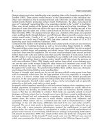
Fig. 13. Sketch of the single sensing element (taxel).

Recently, we proposed a solution based on the scattering of the light illuminating the
surface of urethane foam (De Maria et al., 2008). The configuration makes use of a couple of
emitter/receiver fibres placed at the edge of a micromachined well covered by the foam.
The distance between the two fibres can be chosen in order to ensure a desired sensitivity of
the sensing element. As a demonstration of the effectiveness of the proposed configuration,
we present the results of two sensors, in which the relative distance between the two fibres
was properly selected in order to fit the range of pressures to be detected. Top and lateral
schematic views of a single taxel are shown in Fig. 13. The sensor works as follows: the light
emitted by the illuminating fibre is scattered by the internal surface of the urethane foam
and a fraction of its power is collected by the receiving fibre, depending on the applied
pressure. In particular, when one applies a pressure on the external surface of the urethane
foam, the distance between the tip of the collecting fibre and the internal surface of the foam
is reduced, and this will result in an increased fraction of power collected by the receiving

fibre. The use of a scattering surface, such as that of the urethane foam employed for the
realization of the prototypes, is justified by the fact the multiple scattering permits to
smooth (average-out) local variation of light intensity within the cavity, and thus reduce the
sensitivity of the collected power on micro-displacements of the illuminating and/or
receiving fibre. As the power collected by the receiving fibre is a function of the pressure
applied on the foam surface, it can be used as a measure of the applied force. Obviously, the
collected light is also a function of the relative distance between the illuminating and the
receiving fibres. In our experiments, such a distance was kept constant and was not a
function of the applied force. However, we can exploit such dependence, by choosing an
opportune distance giving rise to a desired sensitivity of the sensor on the applied pressure.
Generally speaking, a smaller distance will result in a higher sensitivity, so that smaller
pressures can be measured.
On the other hand, a higher sensitivity implies a reduced dynamic range, i.e. the sensor
response will saturate at lower pressure levels. Hence, a trade-off must be found between
sensitivity and dynamic range.
One advantage of the proposed technique is that it can be easily extended to a number of
taxels, so as to acquire a pressure distribution. Figure 14 shows a possible configuration of a
matrix of taxels to realize a complete tactile sensor able to detect both contact point and
contact force applied on a finite area.
Two different taxels have been produced with the same well and two different distances
between the emitting/receiving fibres, i.e. 10 m and 200 m. The micromachined well size
is 5x5 mm
2
. The optical source was a superluminescent LED operating at a central
wavelength of 1550nm, and having an output optical power of 3mW. The output pigtail of
Illuminatin
g

Receivin
g

Scatterin
g

Urethane
A
pplied force
Scatterin
g

OpticalFibre,NewDevelopments30

the source was connected to the illuminating fibre, whereas the receiving fibre was
connected to an InGaAs photodiode, whose output signal was fed to an oscilloscope having
an input impedance of 1 M. Both illuminating and receiving fibres were SMF-28, single-
mode optical fibres. The two prototypes have been calibrated with a load cell mounted as
shown in Fig. 15. The results corresponding to the calibration of the first prototype are
reported in Fig. 16 (left), where the output voltage, proportional to the optical power
collected by the receiving fibre, is plotted against the load applied to the sensor. As
expected, the sensitivity is very high but with a limited dynamic range. Moreover, to test the
repeatability of the measurements, different sets of measurements have been collected and
two of them are reported in the figure.

Fig. 14. Schematic diagram of a 10-taxel tactile sensor.

Fig. 15. Experimental set-up for the fibre-optics based taxel.
The second prototype, as expected, had a lower sensitivity but wider dynamic range, as
shown by the calibration curve of Fig. 16 (right). In both cases, the sensitivity is certainly

better than the typical values of commercial optical tactile sensors.

Load cell for calibration Illuminating fibre
Receiving fibre
Tactile sensor
Illuminating fibre
Receiving fibres

5. Conclusions

In this chapter, a number of experimental demonstrations on the use of the optical fibre
sensor technology have been reported. It has been shown that different application fields
can take advantage of the peculiar characteristics of optical fibre sensors. In particular,
distributed fibre sensors have great potentiality in the field of structural health monitoring,
as they permit to perform continuous measurements of the quantity of interest. On the other
hand, fibre Bragg grating technology offers high sensitivity and accuracy, and in general it
benefits from the immunity to electromagnetic interference, in common with other fibre-
optic sensors. Finally, the small size and minimally invasiveness of optical fibres have been
demonstrated to be useful in robotic applications, where the use of fibre-optics may lead to
efficient exteroceptive sensing systems.

Fig. 16. Calibration curves of the first prototype with 10 m distance between the fibres (left)
and of the second prototype with 200 m distance between the fibres (right).

6. References

Agrawal, G.P. (2001). Nonlinear Fibre Optics. Academic Press, San Diego.
Barnoski, J.K. & Jensen, S.M. (1976). Fibre waveguides: A novel technique for investigating

attenuation characteristics. Appl. Opt. Vol. 15, No. 9, 2112-2115.
Bernini, R.; Crocco, L.; Minardo, A.; Soldovieri, F. & Zeni, L. (2002). Frequency-domain
approach to distributed fibre-optic Brillouin sensing. Opt. Lett. Vol. 27, No. 5, 288-
290.
Bernini, R.; Fraldi, M.; Minardo, A.; Minatolo, V.; Carannante, F.; Nunziante, L. & Zeni, L.
(2006a). Identification of defects and strain error estimation for bending steel beams
using time domain Brillouin distributed fibre sensors. Smart Materials and Structures
Vol. 2, 612-622.
Bernini, R.; Minardo, A. & Zeni, L. (2006b). An accurate high resolution technique for
distributed sensing based on frequency domain Brillouin scattering. IEEE Photonics
Technology Letters Vol. 18, No. 1, 280-282.
140 160 180 200 220 240 260 280 300
0
50
100
150
200
250
300
350
Weight [g]
Output Voltage [mV]

Measured
Cubic fitting
Opticalbresinaeronautics,roboticsandcivilengineering 31

the source was connected to the illuminating fibre, whereas the receiving fibre was
connected to an InGaAs photodiode, whose output signal was fed to an oscilloscope having

an input impedance of 1 M. Both illuminating and receiving fibres were SMF-28, single-
mode optical fibres. The two prototypes have been calibrated with a load cell mounted as
shown in Fig. 15. The results corresponding to the calibration of the first prototype are
reported in Fig. 16 (left), where the output voltage, proportional to the optical power
collected by the receiving fibre, is plotted against the load applied to the sensor. As
expected, the sensitivity is very high but with a limited dynamic range. Moreover, to test the
repeatability of the measurements, different sets of measurements have been collected and
two of them are reported in the figure.

Fig. 14. Schematic diagram of a 10-taxel tactile sensor.

Fig. 15. Experimental set-up for the fibre-optics based taxel.
The second prototype, as expected, had a lower sensitivity but wider dynamic range, as
shown by the calibration curve of Fig. 16 (right). In both cases, the sensitivity is certainly
better than the typical values of commercial optical tactile sensors.

Load cell for calibration Illuminating fibre
Receiving fibre
Tactile sensor
Illuminating fibre
Receiving fibres

5. Conclusions

In this chapter, a number of experimental demonstrations on the use of the optical fibre
sensor technology have been reported. It has been shown that different application fields
can take advantage of the peculiar characteristics of optical fibre sensors. In particular,
distributed fibre sensors have great potentiality in the field of structural health monitoring,

as they permit to perform continuous measurements of the quantity of interest. On the other
hand, fibre Bragg grating technology offers high sensitivity and accuracy, and in general it
benefits from the immunity to electromagnetic interference, in common with other fibre-
optic sensors. Finally, the small size and minimally invasiveness of optical fibres have been
demonstrated to be useful in robotic applications, where the use of fibre-optics may lead to
efficient exteroceptive sensing systems.

Fig. 16. Calibration curves of the first prototype with 10 m distance between the fibres (left)
and of the second prototype with 200 m distance between the fibres (right).

6. References

Agrawal, G.P. (2001). Nonlinear Fibre Optics. Academic Press, San Diego.
Barnoski, J.K. & Jensen, S.M. (1976). Fibre waveguides: A novel technique for investigating
attenuation characteristics. Appl. Opt. Vol. 15, No. 9, 2112-2115.
Bernini, R.; Crocco, L.; Minardo, A.; Soldovieri, F. & Zeni, L. (2002). Frequency-domain
approach to distributed fibre-optic Brillouin sensing. Opt. Lett. Vol. 27, No. 5, 288-
290.
Bernini, R.; Fraldi, M.; Minardo, A.; Minatolo, V.; Carannante, F.; Nunziante, L. & Zeni, L.
(2006a). Identification of defects and strain error estimation for bending steel beams
using time domain Brillouin distributed fibre sensors. Smart Materials and Structures
Vol. 2, 612-622.
Bernini, R.; Minardo, A. & Zeni, L. (2006b). An accurate high resolution technique for
distributed sensing based on frequency domain Brillouin scattering. IEEE Photonics
Technology Letters Vol. 18, No. 1, 280-282.
140 160 180 200 220 240 260 280 300
0
50

100
150
200
250
300
350
Weight [g]
Output Voltage [mV]

Measured
Cubic fitting
OpticalFibre,NewDevelopments32

Bernini, R.; Minardo, A.& Zeni, L. (2008). Vectorial dislocation monitoring of pipelines by
use of Brillouin-based fibre-optics sensors. Smart Materials and. Structures. Vol. 17,
015006.
Cavallo, A.; May, C.; Minardo, A.; Natale, C.; Pagliarulo, P. & Pirozzi, P. (2009). Modelling
and control of a smart auxiliary mass damper equipped with a Bragg grating for
active vibration control, Sensors and Actuators A, in press.
Cook, R.O. & Hamm, C.W. (1979). Fibre optic lever displacement transducer. Appl. Opt.
Vol. 18, No. 19, 3230-3241.
Culshaw, B. & Dakin, J. 1997. Optical Fibre sensors Vol. 4. Artech House Publishers,
0890069409.
De Maria, G.; Minardo, A.; Natale, C.; Pirozzi, S. & Zeni, L. (2008). Optoelectronic Tactile
Sensor Based on Micromachined Scattering Wells. FIRST MEDITERRANEAN
PHOTONICS CONFERENCE, European Optical Society Topical Meeting, 25–28
June 2008, Ischia, Italy.
Fields, J.N.; Asawa, C.K.; Ramer, O.G. & Barnowski, M.K. (1980). Fibre Optic Pressure
Sensor. J. Acoust. Soc. Am., Vol. 67, 816-818.

Garus, D.; Krebber, K.; Schliep, F. & Gogolla, T. (1996). Distributed sensing technique based
on Brillouin optical-fibre frequency-domain analysis. Opt. Lett., Vol. 21, No. 17,
1402-1404.
Kersey, A. D.; Davis, M. A.; Patrick, H. J.; LeBlanc, M.; Poo, K. P.; Askins, A.G.; Putnam, M.
A. & Friebele, E. J. (1997). Fibre grating sensors, Journal of Lightw. Technol., vol. 15,
no. 8, pp. 1442-1462.
Krishna, G.M. & Rajanna, K. (2002). Tactile sensor based on piezoelectric resonance. Proc. of
2002 IEEE Conference on Sensor, pp. 1643- 1647.
Liu, L.; Zheng, X. & Li, Z. (1993). An array tactile sensor with piezoresistive with single
crystal silicon diaphragm. Sensors and Actuators-A32, 193-196.
Maekawa, H.; Tanie, K. & Komoriya, K. (1993). A finger-shaped tactile sensor using an
optical waveguide. Proc. of 1993 IEEE International Conference on Systems, Man and
Cybernetics, pp. 403-408.
Measures, R.M. (2002). Structural monitoring with fibre optic technology. Academic press, San
Diego.
Morimura, H.; Shigematsu, S. & Machinda, K. (2000). A novel sensor cell architecture and
sensing circuit scheme for capacitive fingerprint sensors. IEEE Journal of Solid State
Circuits, Vol, 35, 724-731.
May, C.; Pagliarulo, P. & Janocha, H. (2006). Optimisation of a magnetostrictive auxiliary
mass damper. Proc. 10th International Conference on New Actuators ACTUATOR2006,
Bremen, Germany, pp. 344–348.
Nikles, M.; Thevenaz, L. & Robert, P.A. 1997. Brillouin gain spectrum characterization in
single-mode optical fibres. J. Lightw. Technol., Vol. 15, No. 10, 1842 – 1851.
Ohka, M.; Kobayashi, H.; Takata, J. & Mitsuya, Y. (2006). Sensing Precision of an Optical
Three-axis Tactile Sensor for a Robotic Finger. Proc. Of the 15th IEEE International
Symposium on Robot and Human Interactive Communication, pp. 214-219.
Rossiter, J. & Mukai, T. (2005). A novel tactile sensor using a matrix of LEDs operating in
both photoemitter and photodetector modes. Proc. of 2005 IEEE Conference on
Sensor, pp. 994-997.

Saran, A.; Abeysinghe, D.C. & Boyd, J.T. (2006. Microelectromechanical system pressure
sensor integrated onto optical fibre by anodic bonding. Appl. Opt., Vol. 45, 1737-
1742.
Tanie, K. (1986). Advances in tactile sensors for robotics. Proc. of the 6th Sensor Symposium
Japan, pp. 63-68.
Udd. E. (2002). Overview of fibre optic sensors, In: Fibre Optic Sensors. Francis T. S. Yu;
Shizhuo Yin, pp. 1-40, Routledge, 978-0-203-90946-1, USA.
Wang, A.; Xiao, H.; Wang, J.; Wang, Z.; Zhao, W. & May, R.G. (2001). Self-calibrated
interferometric-based-optical fibre sensors. J. Lightw. Technol., Vol. 19, No. 10, 1495-
1501.
Yuan, S.; Ansari, F.; Liu, X. & Zhao, Y. (2005). Optical fibre based dynamic pressure sensor
for WIM sensor. Sens. and Actuat. A, Vol. 120, No. 1, 53-58.
Zhao, Y. & Liao, Y. (2004) “Discrimination methods and demodulation techniques for fibre
Bragg grating sensors”, Opt. Lasers Eng., vol. 41, pp. 1-18.

Opticalbresinaeronautics,roboticsandcivilengineering 33

Bernini, R.; Minardo, A.& Zeni, L. (2008). Vectorial dislocation monitoring of pipelines by
use of Brillouin-based fibre-optics sensors. Smart Materials and. Structures. Vol. 17,
015006.
Cavallo, A.; May, C.; Minardo, A.; Natale, C.; Pagliarulo, P. & Pirozzi, P. (2009). Modelling
and control of a smart auxiliary mass damper equipped with a Bragg grating for
active vibration control, Sensors and Actuators A, in press.
Cook, R.O. & Hamm, C.W. (1979). Fibre optic lever displacement transducer. Appl. Opt.
Vol. 18, No. 19, 3230-3241.
Culshaw, B. & Dakin, J. 1997. Optical Fibre sensors Vol. 4. Artech House Publishers,
0890069409.
De Maria, G.; Minardo, A.; Natale, C.; Pirozzi, S. & Zeni, L. (2008). Optoelectronic Tactile
Sensor Based on Micromachined Scattering Wells. FIRST MEDITERRANEAN
PHOTONICS CONFERENCE, European Optical Society Topical Meeting, 25–28

June 2008, Ischia, Italy.
Fields, J.N.; Asawa, C.K.; Ramer, O.G. & Barnowski, M.K. (1980). Fibre Optic Pressure
Sensor. J. Acoust. Soc. Am., Vol. 67, 816-818.
Garus, D.; Krebber, K.; Schliep, F. & Gogolla, T. (1996). Distributed sensing technique based
on Brillouin optical-fibre frequency-domain analysis. Opt. Lett., Vol. 21, No. 17,
1402-1404.
Kersey, A. D.; Davis, M. A.; Patrick, H. J.; LeBlanc, M.; Poo, K. P.; Askins, A.G.; Putnam, M.
A. & Friebele, E. J. (1997). Fibre grating sensors, Journal of Lightw. Technol., vol. 15,
no. 8, pp. 1442-1462.
Krishna, G.M. & Rajanna, K. (2002). Tactile sensor based on piezoelectric resonance. Proc. of
2002 IEEE Conference on Sensor, pp. 1643- 1647.
Liu, L.; Zheng, X. & Li, Z. (1993). An array tactile sensor with piezoresistive with single
crystal silicon diaphragm. Sensors and Actuators-A32, 193-196.
Maekawa, H.; Tanie, K. & Komoriya, K. (1993). A finger-shaped tactile sensor using an
optical waveguide. Proc. of 1993 IEEE International Conference on Systems, Man and
Cybernetics, pp. 403-408.
Measures, R.M. (2002). Structural monitoring with fibre optic technology. Academic press, San
Diego.
Morimura, H.; Shigematsu, S. & Machinda, K. (2000). A novel sensor cell architecture and
sensing circuit scheme for capacitive fingerprint sensors. IEEE Journal of Solid State
Circuits, Vol, 35, 724-731.
May, C.; Pagliarulo, P. & Janocha, H. (2006). Optimisation of a magnetostrictive auxiliary
mass damper. Proc. 10th International Conference on New Actuators ACTUATOR2006,
Bremen, Germany, pp. 344–348.
Nikles, M.; Thevenaz, L. & Robert, P.A. 1997. Brillouin gain spectrum characterization in
single-mode optical fibres. J. Lightw. Technol., Vol. 15, No. 10, 1842 – 1851.
Ohka, M.; Kobayashi, H.; Takata, J. & Mitsuya, Y. (2006). Sensing Precision of an Optical
Three-axis Tactile Sensor for a Robotic Finger. Proc. Of the 15th IEEE International
Symposium on Robot and Human Interactive Communication, pp. 214-219.
Rossiter, J. & Mukai, T. (2005). A novel tactile sensor using a matrix of LEDs operating in

both photoemitter and photodetector modes. Proc. of 2005 IEEE Conference on
Sensor, pp. 994-997.

Saran, A.; Abeysinghe, D.C. & Boyd, J.T. (2006. Microelectromechanical system pressure
sensor integrated onto optical fibre by anodic bonding. Appl. Opt., Vol. 45, 1737-
1742.
Tanie, K. (1986). Advances in tactile sensors for robotics. Proc. of the 6th Sensor Symposium
Japan, pp. 63-68.
Udd. E. (2002). Overview of fibre optic sensors, In: Fibre Optic Sensors. Francis T. S. Yu;
Shizhuo Yin, pp. 1-40, Routledge, 978-0-203-90946-1, USA.
Wang, A.; Xiao, H.; Wang, J.; Wang, Z.; Zhao, W. & May, R.G. (2001). Self-calibrated
interferometric-based-optical fibre sensors. J. Lightw. Technol., Vol. 19, No. 10, 1495-
1501.
Yuan, S.; Ansari, F.; Liu, X. & Zhao, Y. (2005). Optical fibre based dynamic pressure sensor
for WIM sensor. Sens. and Actuat. A, Vol. 120, No. 1, 53-58.
Zhao, Y. & Liao, Y. (2004) “Discrimination methods and demodulation techniques for fibre
Bragg grating sensors”, Opt. Lasers Eng., vol. 41, pp. 1-18.

OpticalFibre,NewDevelopments34
OpticalFibreSensorSystemforMultipointCorrosionDetection 35
OpticalFibreSensorSystemforMultipointCorrosionDetection
JoaquimF.Martins-FilhoandEduardoFontana
X

Optical Fibre Sensor System for
Multipoint Corrosion Detection

Joaquim F. Martins-Filho and Eduardo Fontana
Department of Electronics and Systems, Federal University of Pernambuco
Brazil

1. Introduction

Over the past thirty years there has been intense research and development on optical fibre
sensors for many applications, basically because of their advantages over other technologies,
such as immunity to electromagnetic interference, lightweight, small size, high sensitivity,
large bandwidth, and ease in signal light transmission. The applications include sensing
temperature, strain, pressure, current/voltage, chemical/gas, displacement, and biological
processes among others. To accomplish those, different optical technologies have been
employed such as fibre grating, interferometry, light scattering and reflectometry, Faraday
rotation, luminescence and others. A review on fibre sensors can be found in (Lee, 2003).
Corrosion and its effects have a profound impact on the infrastructure and equipment of
countries worldwide. This impact is manifested in significant maintenance, repair, and
replacement efforts; reduced access, availability and production; poor performance; high
environmental risks; and unsafe conditions associated with facilities and equipment. There
have been some efforts from different countries to estimate the cost of corrosion and the
results indicate that it can reach 2 to 5% of the gross national product. For example,
corrosion damage represented an estimated cost of US$ 276 billions in the United States of
America in 2002 (Thompson et al., 2005). Therefore, corrosion monitoring is an important
aspect of modern infrastructure in industry sectors such as mining, aircraft, shipping,
oilfields, as well as in military and civil facilities.
Optical fibre-based corrosion sensors have been investigated in recent years mainly because
of the advantages obtained by the use of optical fibres, as already pointed out. A short
review of the technologies employed in the fibre-based corrosion sensors can be found in
(Wade et al., 2008). The reported applications include corrosion monitoring in aircrafts
(Benounis & Jaffrezic-Renault, 2004), in the concrete of roadways and bridges (Fuhr &
Huston, 1998) and in oilfields.

2. Corrosion Monitoring in Deepwater Oilfield Pipelines

In the oil industry, to which we focus the sensing approach described in this chapter, a very
challenging problem is that related to surveillance and maintenance of deepwater oilfield
pipelines, given the harsh environment to be monitored and the long distances involved.
3
OpticalFibre,NewDevelopments36

These structures are subject to corrosion and sand-induced erosion in a high pressure, high
temperature environment. Moreover, the long distances (kilometres) between the corrosion
points and the monitoring location make the commercially available instruments not
appropriate for monitoring these pipelines. Costly, regularly scheduled, preventive
maintenance is then required (Staveley, 2004; Yin et al., 2000). Electronic and
electromagnetic-based corrosion sensors (Yin et al., 2000; Vaskivsky et al., 2001; Andrade
Lima et al., 2001) are also not suitable in these conditions. Fibre optic based corrosion
sensors are ideal for this application. However, the sensing approaches reported in the
literature are either single point (Qiao et al., 2006; Wade et al., 2008) or use a stripped
cladding fibre structure that requires a high precision mechanical positioning system with
moving parts for light detection, which compromises the robustness of the sensor system
(Benounis et al., 2003; Benounis & Jaffrezic-Renault, 2004; Saying et al., 2006; Cardenas-
Valencia et al., 2007). An optical fibre PH sensor has been recently developed for the indirect
evaluation of the corrosion process in petroleum wells (Da Silva Jr. et al., 2007). It employs a
fibre Bragg grating mechanically coupled to a PH-sensitive hydrogel, which changes its
volume according to the PH of the medium. Thus, the change in PH is translated into a
mechanical strain on the Bragg grating, which can be interrogated by standard optical
methods. Although it can easily be multiplexed for multipoint measurements, this technique
is limited to the evaluation of the chemical corrosion due to acid attack inside the well,
disregarding the combined effects of other important sources of corrosion, such as
mechanical (erosion), chemical, thermic and biological (microorganisms). The oil industry
can also make use of the time domain reflectometry (TDR) technique to evaluate the
corrosion process inside pipelines and oil wells (Kohl, 2000). The proposed scheme involves
the deployment of a metallic cable inside and along the pipeline or well. The conductor is

exposed to the fluid at selected locations such that it should be susceptible to the same
corrosive processes as the pipeline. A signal generator launches a pulsed electrical signal to
the conductor cable and an electronic receiver measures the reflected pulses intensity and
delay. The reflections come from the locations where the exposed cable was affected by the
corrosion process, which changes its original impedance. This TDR technique has also been
applied to the monitoring of corrosion in steel cables of bridges (Liu et al., 2002). Although
this technique has the advantage of being multipoint or even distributed, it is limited in
reach. For practical purposes the maximum distance covered by the sensor is about 2 km.
This is suitable for standard wells, but not for deep oilfields, especially those from the
recently discovered presalt regions in Brazil, which are over 6 km deep.

3. A Multipoint Fibre Optic Corrosion Sensor

We have recently presented for the first time the concept and first experimental results of a
fibre-optic-based corrosion sensor using the optical time domain reflectometry (OTDR)
technique as the interrogation method (Martins-Filho et al., 2007; Martins-Filho et al., 2008).
Our proposed sensor system is multipoint, self-referenced, has no moving parts and can
detect the corrosion rate several kilometres away from the OTDR equipment. These features
make it very suitable to the problem of corrosion monitoring of deepwater pipelines in the
oil industry. It should be pointed out, however, that the approach is not limited to this
specific application and can be employed to address a number of single or multipoint
corrosion detection problems in other industrial sectors.

In this chapter we present a detailed description of the sensor system, further experimental
results and theoretical calculations for the measurement of the corrosion rate of aluminium
films in controlled laboratory conditions and also for the evaluation of the maximum
number of sensor heads the system supports.

3.1 Sensor Setup
Our proposed sensor system consists of several sensor heads connected to a commercial

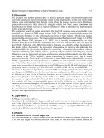
OTDR equipment by a single-mode optical fibre and fibre couplers. Figure 1 shows the
corrosion sensor setup. The OTDR is connected to a 2 km long single mode optical fibre.
Directional couplers can split the optical signal such that a small fraction (3 to 9%) is
directed to the sensing heads. The OTDR operates at 1.55 m, with a pulsewidth of 10 ns,
which corresponds to a spatial resolution of 2 m. The OTDR is set to measure 50000 points
for the total distance of 5 km (one point every 10 cm). The optical fibres and couplers are
standard telecommunication devices. The sensor heads have 100 nm of aluminium
deposited on cleaved fibre facets by a standard thermal evaporation process and they are
numbered from 1 to 11 in Fig. 1.
Fig. 1. Schematic diagram of the corrosion sensor. Sensor heads are numbered. Fibre lengths
and split ratios are shown.

3.2 Results
For laboratory measurements the corrosion action was simulated by controlled etching of
the Aluminium film on the sensor head. We used 25 H
3
PO
4
: 1 HNO
3
: 5 CH
3
COOH as the
Al-etcher. The expected corrosion rate of Al from this etcher is 50 nm/min. Figure 2-a shows
the OTDR trace where each peak, numbered from 1 to 11, indicates the reflection from the
corresponding sensing head. The head number 6 is immersed in the Al-etcher. As the
aluminium is being removed from the fibre facet the reflected light measured in the OTDR
decreases, as shown in Fig. 2-b.
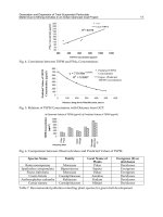
In Fig. 3 we plot the ratio of peak (point A) to valley (point B) of the reflected light shown in
Fig. 2-b as a function of the aluminium corrosion time. Figure 3 shows that up to 60 seconds

of corrosion there is no significant change in the OTDR measured reflected light, since the
aluminium is still too thick. Further up from this point the reflection drops to a minimum
and then stabilizes at a constant level. The constant level means that the corrosion process
on the fibre facet has ended. We obtain the corrosion rate by taking the deposited metal
thickness and the time taken to reach the constant level, as show in Fig. 3.
40m40m40m40m40m40m 40m40m40m40m
10m10m10m10m10m10m 10m10m10m10m
4
96
5
95
7
93
7
93
6
94
6
94
5
95
9
91
8
92
3
97
1 2
3
4 5 6 7 8 9 10

OTDR
11
Optical Fiber
2km
OpticalFibreSensorSystemforMultipointCorrosionDetection 37

These structures are subject to corrosion and sand-induced erosion in a high pressure, high
temperature environment. Moreover, the long distances (kilometres) between the corrosion
points and the monitoring location make the commercially available instruments not
appropriate for monitoring these pipelines. Costly, regularly scheduled, preventive
maintenance is then required (Staveley, 2004; Yin et al., 2000). Electronic and
electromagnetic-based corrosion sensors (Yin et al., 2000; Vaskivsky et al., 2001; Andrade
Lima et al., 2001) are also not suitable in these conditions. Fibre optic based corrosion
sensors are ideal for this application. However, the sensing approaches reported in the
literature are either single point (Qiao et al., 2006; Wade et al., 2008) or use a stripped
cladding fibre structure that requires a high precision mechanical positioning system with
moving parts for light detection, which compromises the robustness of the sensor system
(Benounis et al., 2003; Benounis & Jaffrezic-Renault, 2004; Saying et al., 2006; Cardenas-
Valencia et al., 2007). An optical fibre PH sensor has been recently developed for the indirect
evaluation of the corrosion process in petroleum wells (Da Silva Jr. et al., 2007). It employs a
fibre Bragg grating mechanically coupled to a PH-sensitive hydrogel, which changes its
volume according to the PH of the medium. Thus, the change in PH is translated into a
mechanical strain on the Bragg grating, which can be interrogated by standard optical
methods. Although it can easily be multiplexed for multipoint measurements, this technique
is limited to the evaluation of the chemical corrosion due to acid attack inside the well,
disregarding the combined effects of other important sources of corrosion, such as
mechanical (erosion), chemical, thermic and biological (microorganisms). The oil industry
can also make use of the time domain reflectometry (TDR) technique to evaluate the
corrosion process inside pipelines and oil wells (Kohl, 2000). The proposed scheme involves
the deployment of a metallic cable inside and along the pipeline or well. The conductor is

OTDR
11
Optical Fiber
2km
OpticalFibre,NewDevelopments38


2.0 2.1 2.2 2.3 2.4 2.5 2.6
0
10
20
30
40
50

Intensity (dB)
Distance (Km)
(a)
1
2
3
4
5
6
7
8
9
10
11

2,338 2,340 2,342 2,344 2,346 2,348 2,350 2,352 2,354 2,356
15
20
25
30
35
40
45
Intensity (dB)
Distance (Km)
Corrosion
Time (s)
68.5
76.9
82.0
84.4
87.6
91.4
94.8
B
A
(b)

Fig. 2. (a) OTDR trace, corresponding to the intensity of the reflected light as a function of
distance along the fibre. Sensor head numbers are shown. (b) OTDR traces for sensor head
number 6, for several corrosion times.

The measured corrosion rate was 47.5 nm/min, which is very close to the expected value (50
nm/min). Other measurements performed using different sensor heads showed similar

results. It is important to note that since the corrosion rate is obtained from the ratio of peak
(point A) to valley (point B) of the OTDR trace as a function of time, this measurement is
self-referenced, because the ratio is immune, to a certain extent, to small optical power
fluctuations that may occur due to changes in the OTDR signal power, optical fibre and fibre
coupler loss variations along the sensor system.
0 20 40 60 80 100 120 140
4
6
8
10
12
14
16
18
20
22
24
Relative Intensity (dB)
Corrosion Time (s)
Corrosion Rate
Metal
Thickness
0
100nm

Fig. 3. Relative intensity obtained from Fig. 2-b, as a function of the corrosion time. Metal
thickness and corrosion rate are shown.

Figure 3 also shows a valley in the relative reflected intensity just before the constant level
used for corrosion determination. Although this feature does not seem to be important for

the determination of the corrosion rate, we verified if it would be an artifact due to the
pulsed OTDR operation in the multipoint (multireflection) setup scheme shown in Fig.1, by
performing measurements in the single head setup show in Fig. 4. This new setup uses a
CW laser source and an optical power meter, instead of the OTDR. The laser light at 1.55 m
from the CW laser with fibre pigtail is coupled to an optical isolator and then to a 50%
coupler and to a 79/21 coupler. The output of this coupler has another optical isolator in one
end and a sensor head in the other end. The sensor head used here is similar to those used in
the multipoint setup of Fig. 1. The light reflected from the sensor head reaches the optical
power meter through the optical couplers. The two isolators avoid unwanted reflections to
reach the power meter and the laser source, which could cause interference effects and
instabilities. For corrosion measurements we used the same Aluminium etcher as described
before. Figure 5 shows the optical power as a function of the corrosion time obtained from
the single head setup of Fig. 4. This result also exhibits the valley observed in the multipoint
setup that uses the OTDR (Fig. 3), indicating that this feature is not a measurement artifact.
Also, Fig. 5 confirms the corrosion rate obtained from Fig. 3, since the constant level starts at
about 120 seconds of corrosion.
OpticalFibreSensorSystemforMultipointCorrosionDetection 39


2.0 2.1 2.2 2.3 2.4 2.5 2.6
0
10
20
30
40
50

Intensity (dB)
Distance (Km)

(a)
1
2
3
4
5
6
7
8
9
10
11

2,338 2,340 2,342 2,344 2,346 2,348 2,350 2,352 2,354 2,356
15
20
25
30
35
40
45
Intensity (dB)
Distance (Km)
Corrosion
Time (s)
68.5
76.9
82.0
84.4
87.6

91.4
94.8
B
A
(b)

Fig. 2. (a) OTDR trace, corresponding to the intensity of the reflected light as a function of
distance along the fibre. Sensor head numbers are shown. (b) OTDR traces for sensor head
number 6, for several corrosion times.

The measured corrosion rate was 47.5 nm/min, which is very close to the expected value (50
nm/min). Other measurements performed using different sensor heads showed similar
results. It is important to note that since the corrosion rate is obtained from the ratio of peak
(point A) to valley (point B) of the OTDR trace as a function of time, this measurement is
self-referenced, because the ratio is immune, to a certain extent, to small optical power
fluctuations that may occur due to changes in the OTDR signal power, optical fibre and fibre
coupler loss variations along the sensor system.
0 20 40 60 80 100 120 140
4
6
8
10
12
14
16
18
20
22
24
Relative Intensity (dB)

Corrosion Time (s)
Corrosion Rate
Metal
Thickness
0
100nm

Fig. 3. Relative intensity obtained from Fig. 2-b, as a function of the corrosion time. Metal
thickness and corrosion rate are shown.

Figure 3 also shows a valley in the relative reflected intensity just before the constant level
used for corrosion determination. Although this feature does not seem to be important for
the determination of the corrosion rate, we verified if it would be an artifact due to the
pulsed OTDR operation in the multipoint (multireflection) setup scheme shown in Fig.1, by
performing measurements in the single head setup show in Fig. 4. This new setup uses a
CW laser source and an optical power meter, instead of the OTDR. The laser light at 1.55 m
from the CW laser with fibre pigtail is coupled to an optical isolator and then to a 50%
coupler and to a 79/21 coupler. The output of this coupler has another optical isolator in one
end and a sensor head in the other end. The sensor head used here is similar to those used in
the multipoint setup of Fig. 1. The light reflected from the sensor head reaches the optical
power meter through the optical couplers. The two isolators avoid unwanted reflections to
reach the power meter and the laser source, which could cause interference effects and
instabilities. For corrosion measurements we used the same Aluminium etcher as described
before. Figure 5 shows the optical power as a function of the corrosion time obtained from
the single head setup of Fig. 4. This result also exhibits the valley observed in the multipoint
setup that uses the OTDR (Fig. 3), indicating that this feature is not a measurement artifact.
Also, Fig. 5 confirms the corrosion rate obtained from Fig. 3, since the constant level starts at
about 120 seconds of corrosion.
OpticalFibre,NewDevelopments40

CW Laser
Coupler
50/50
Coupler
79/21
Isolator Isolator
Power
Meter
Sensor
Head

Fig. 4. Schematic diagram of the single head setup.

0 50 100 150 200
-60
-50
-40
-30
-20
-10
Power (dBm)
Time (s)

Fig. 5. Reflected optical power from a single head setup as a function of the corrosion time.

We also used the Fresnel reflection formulation (Fontana & Pantell, 1988) for a silica-Al-
liquid single layer structure, as shown in Fig. 6, to study the reflection properties of the
sensing head. Neglecting the small beam divergence of the guided mode, the reflectance is
given by



 
2
202312
202312
2exp1
2exp
dkjrr
dkjrr
R



, (1)
where
ii
ii
ii
r






1
1
1,
(2)

is the normal incidence reflectivity at the interface between media i and i+1 (i = 1, 2), k
0
=
2π/λ, ε
i
is the relative electrical permittivity of medium i (i = 1, 2, 3) and d is the metal film
thickness.

We assumed that the etching solution had a refractive index close to that of pure water, for
the sake of simplicity. Optical parameters for silica (Malitson, 1965), pure water (Schiebener
et al., 1990) and Al (Lide, 2004) at  = 1.55 m were used in the calculations.

fiber core
fiber cladding
Medium 1
(fiber) 

Medium 2
(aluminum) 

Medium 3
(liquid) 

d

Fig. 6. Schematic diagram of the sensing head showing the Aluminium film of thickness d
on the fibre facet.

Figure 7 shows a theoretical simulation as well as the experimental data for the reflectance
at the metalized fibre facet as a function of the metal film thickness. The experimental data

were obtained from Fig. 5. The theoretical result showed no evidence of a minimum
reflectance with the strong depth observed experimentally at an estimated Al film thickness
of 15 nm. In fact, the theoretical prediction yields almost 100% reflectance at this thickness
value, as can be noticed in Fig. 7. The difference between theoretical and experimental
results indicates that the valley observed in the experimental results is not due to any
interference effect that could occur in the fibre-metal-liquid interfaces.
Due to the resonant nature of the reflectance minima shown in Figs. 3 and 5, it is very likely
that they occur due to roughness induced, resonant coupling to surface plasmons (Fontana
& Pantell, 1988) at the metal-liquid interface as a thin and rough layer of metal may result
during the etching process. The coupling is thickness dependent and the strength depends
on the average size of irregularities on the surface (Fontana & Pantell, 1988). Given that the
dispersion relation of surface plasmons is very near that of photons in this spectral region,
surface roughness could provide the required small increase in momentum for efficient
coupling to the surface plasmon oscillation. A more elaborated calculation will be
performed in future work taking into account the change in dispersion relation of surface
plasmons due to roughness (Fontana & Pantell, 1988), to account for this effect.
It is worth noticing from Fig. 7 that the reflectance predicted theoretically with no metal film
was 26.7 dB lower than that at maximum thickness, a result that differs significantly from
the drop of  14 dB observed experimentally in Fig. 3 and  35 dB in Fig. 7. This is probably
due to the residual clusters left on the fibre facet that form an absorbing, non-homogeneous
interface that changes the reflectance relative to that predicted theoretically for a single
glass-liquid interface. In fact we observed from a direct inspection with an optical
microscope that some clusters of material still remained on the fibre facet, which were no
longer affected by the Al-etcher. As can be seen from Figs. 3 and 7, the resonant features in
the experimental results are similar, although the minima occur at different time points.
There is, however, a significant difference from 14 to 35 dB in the final reflectance drop
obtained from the data of Figs. 3 and 7, respectively, which may be due to the distinct
procedures used to carry out the experiments. For the data shown in Fig. 3, obtained with
OpticalFibreSensorSystemforMultipointCorrosionDetection 41


 
2
202312
202312
2exp1
2exp
dkjrr
dkjrr
R



, (1)
where
ii
ii
ii
r






1
1
1,
(2)

the OTDR, since the equipment is somewhat slow to execute several measurements to
average them in time, the head was placed in the etcher for a given time and then in water
for OTDR reading and averaging for each data point. For the case of Fig. 7, we used the
single head setup of Fig. 4, and we attempted to avoid artifacts introduced by the use of
alternate solutions and employed an optical power meter for fast data reading and
averaging, and thus the sensor head could remain immersed in the etcher during the entire
measurement. These distinct procedures may lead to different residual clustering in the fibre
facets, which can be the cause of the difference in the results of Figs. 3 and 7. It will be
further investigated in the future.













50 60 70 80 90 100
Al thickness (nm)
Theory
Data
10log(
R
)
60

40
30 20 10 0

Fig. 7. Theoretical (line) and experimental data (dots) for the reflectance as a function of the
Aluminium film thickness.

We also evaluated experimentally the maximum number of sensor heads our sensor system
can support, and we found that it depends on the dynamic range of the OTDR. For the
OTDR pulsewidth used to obtain the results shown here (10 ns) its dynamic range is about 7
dB. Since each coupler has an insertion loss of about 0.7 dB, we can have up to 10 sensor
heads in this configuration. This can be verified from Fig. 2-a. One can see that as the
number of heads increases along the fibre length the OTDR trace becomes noisier. This
noisy trace should have impact on the accuracy of the measured corrosion rate for the heads
located further away from the OTDR. On the other hand, for 500 ns pulsewidth the OTDR
dynamic range is 20.4 dB, which allows the use of up to 30 sensing heads. In this case the
OTDR spatial resolution is about 100 m. Therefore, the minimum separation between
consecutive sensor heads should be of about 200 m. In this configuration the sensor system
would cover a total length of 6 km, with a sensor head every 200 meters.

4. Conclusions

We proposed and demonstrated experimentally an optical fibre sensor for the corrosion
process in metal (Aluminium) using the optical time domain reflectometry technique. We

presented experimental results for the measurement of the corrosion rate of aluminium
films in controlled laboratory conditions. The obtained corrosion rate matched the expected
rate of the etcher used. We also evaluated experimentally the maximum number of sensor
heads the system supports. It depends on the OTDR dynamic range and it has implications
on the distance between consecutive sensor heads.
Our proposed sensor system is multipoint, self-referenced, has no moving parts (all-fibre)

and can detect the corrosion rate for each head several kilometres away from the OTDR,
thus making the system ideal for “in-the-field” monitoring of corrosion and erosion. This
system may have applications in harsh environments such as in deepwater oil wells and gas
flowlines (including from the presalt region), for the evaluation of the corrosion and erosion
processes in the inner wall of the casing pipes. In this case, different materials can be
deposited on the fibre facet to better match the pipe materials under corrosion/erosion. This
system may enable inferred condition-based maintenance without production interruption,
decreasing the cost of oil production, and substantially reducing the risk of environmental
disasters due to the failure of unmonitored flowlines.
Our experimental results also revealed a feature that may indicate the occurrence of the
surface plasmon effect at the metal-liquid interface. It could be due to the roughness
coupling to surface plasmons at the metal-liquid interface as a thin and rough layer of metal
may result during the etching process. Although we believe at this point that this effect is
not vital for the operation of the proposed sensor, nor to the measurement of the corrosion
rate, it will be investigated in future work.

5. References

Andrade Lima, E. & Bruno, A. C. (2001). Improving the Detection of Flaws in Steel Pipes
Using SQUID Planar Gradiometers. IEEE Transactions on Applied Superconductivity,
Vol. 11, No. 1, Mar 2001, 1299-1302, ISSN 1051-8223.
Benounis, M.; Jaffrezic-Renault, N.; Stremsdoerfer, G. & Kherrat, R. (2003). Elaboration and
standardization of an optical fibre corrosion sensor based on an electroless deposit
of copper. Sensors and Actuators B, Vol. 90, 2003, 90-97, ISSN 0925-4005.
Benounis, M. & Jaffrezic-Renault, N. (2004). Elaboration of an optical fibre corrosion sensor
for aircraft applications. Sensors and Actuators B, Vol. 100, March 2004, 1-8, ISSN
0925-4005
Cardenas-Valencia, A. M.; Byrne, R. H.; Calves, M.; Langebrake, L.; Fries, D. P. & Steimle, E.
T. (2007). Development of stripped-cladding optical fiber sensors for continuous
monitoring II: Referencing method for spectral sensing of environmental corrosion.

Sensors and Actuators B, Vol. 122, 2007, 410-418, ISSN 0925-4005
Da Silva Jr., M. F.; D'almeida, A. R.; Ribeiro, F. P.; Valente, L. C. G.; Braga, A. M. B. &
Triques, A. L. C. (2007). Optical Fiber PH Sensor, US Patent no. 7251384, granted in
July 2007, available in
Fontana, E. & Pantell, R. H. (1988). Characterization of multilayer rough surfaces by use of
surface-plasmon spectroscopy. Physical Review B, Vol. 37, No. 7, 1988, 3164-3182,
ISSN 0163-1829.
Fuhr, P. L. & Huston, D. R. (1998). Corrosion detection in reinforced concrete roadways and
bridges via embedded fiber optic sensors, Smart Materials and Structures, Vol. 7,
1998, pp. 217–228, ISSN 0964-1726.
OpticalFibreSensorSystemforMultipointCorrosionDetection 43

the OTDR, since the equipment is somewhat slow to execute several measurements to
average them in time, the head was placed in the etcher for a given time and then in water
for OTDR reading and averaging for each data point. For the case of Fig. 7, we used the
single head setup of Fig. 4, and we attempted to avoid artifacts introduced by the use of
alternate solutions and employed an optical power meter for fast data reading and
averaging, and thus the sensor head could remain immersed in the etcher during the entire
measurement. These distinct procedures may lead to different residual clustering in the fibre
facets, which can be the cause of the difference in the results of Figs. 3 and 7. It will be
further investigated in the future.














50 60 70 80 90 100
Al thickness (nm)
Theory
Data
10log(
R
)
60
40
30 20 10 0

Fig. 7. Theoretical (line) and experimental data (dots) for the reflectance as a function of the
Aluminium film thickness.

We also evaluated experimentally the maximum number of sensor heads our sensor system
can support, and we found that it depends on the dynamic range of the OTDR. For the
OTDR pulsewidth used to obtain the results shown here (10 ns) its dynamic range is about 7
dB. Since each coupler has an insertion loss of about 0.7 dB, we can have up to 10 sensor
heads in this configuration. This can be verified from Fig. 2-a. One can see that as the
number of heads increases along the fibre length the OTDR trace becomes noisier. This
noisy trace should have impact on the accuracy of the measured corrosion rate for the heads
located further away from the OTDR. On the other hand, for 500 ns pulsewidth the OTDR
dynamic range is 20.4 dB, which allows the use of up to 30 sensing heads. In this case the
OTDR spatial resolution is about 100 m. Therefore, the minimum separation between
consecutive sensor heads should be of about 200 m. In this configuration the sensor system
would cover a total length of 6 km, with a sensor head every 200 meters.

4. Conclusions

We proposed and demonstrated experimentally an optical fibre sensor for the corrosion
process in metal (Aluminium) using the optical time domain reflectometry technique. We

presented experimental results for the measurement of the corrosion rate of aluminium
films in controlled laboratory conditions. The obtained corrosion rate matched the expected
rate of the etcher used. We also evaluated experimentally the maximum number of sensor
heads the system supports. It depends on the OTDR dynamic range and it has implications
on the distance between consecutive sensor heads.
Our proposed sensor system is multipoint, self-referenced, has no moving parts (all-fibre)
and can detect the corrosion rate for each head several kilometres away from the OTDR,
thus making the system ideal for “in-the-field” monitoring of corrosion and erosion. This
system may have applications in harsh environments such as in deepwater oil wells and gas
flowlines (including from the presalt region), for the evaluation of the corrosion and erosion
processes in the inner wall of the casing pipes. In this case, different materials can be
deposited on the fibre facet to better match the pipe materials under corrosion/erosion. This
system may enable inferred condition-based maintenance without production interruption,
decreasing the cost of oil production, and substantially reducing the risk of environmental
disasters due to the failure of unmonitored flowlines.
Our experimental results also revealed a feature that may indicate the occurrence of the
surface plasmon effect at the metal-liquid interface. It could be due to the roughness
coupling to surface plasmons at the metal-liquid interface as a thin and rough layer of metal
may result during the etching process. Although we believe at this point that this effect is
not vital for the operation of the proposed sensor, nor to the measurement of the corrosion
rate, it will be investigated in future work.

5. References

Andrade Lima, E. & Bruno, A. C. (2001). Improving the Detection of Flaws in Steel Pipes
Using SQUID Planar Gradiometers. IEEE Transactions on Applied Superconductivity,
Vol. 11, No. 1, Mar 2001, 1299-1302, ISSN 1051-8223.
Benounis, M.; Jaffrezic-Renault, N.; Stremsdoerfer, G. & Kherrat, R. (2003). Elaboration and
standardization of an optical fibre corrosion sensor based on an electroless deposit
of copper. Sensors and Actuators B, Vol. 90, 2003, 90-97, ISSN 0925-4005.
Benounis, M. & Jaffrezic-Renault, N. (2004). Elaboration of an optical fibre corrosion sensor
for aircraft applications. Sensors and Actuators B, Vol. 100, March 2004, 1-8, ISSN
0925-4005
Cardenas-Valencia, A. M.; Byrne, R. H.; Calves, M.; Langebrake, L.; Fries, D. P. & Steimle, E.
T. (2007). Development of stripped-cladding optical fiber sensors for continuous
monitoring II: Referencing method for spectral sensing of environmental corrosion.
Sensors and Actuators B, Vol. 122, 2007, 410-418, ISSN 0925-4005
Da Silva Jr., M. F.; D'almeida, A. R.; Ribeiro, F. P.; Valente, L. C. G.; Braga, A. M. B. &
Triques, A. L. C. (2007). Optical Fiber PH Sensor, US Patent no. 7251384, granted in
July 2007, available in
Fontana, E. & Pantell, R. H. (1988). Characterization of multilayer rough surfaces by use of
surface-plasmon spectroscopy. Physical Review B, Vol. 37, No. 7, 1988, 3164-3182,
ISSN 0163-1829.
Fuhr, P. L. & Huston, D. R. (1998). Corrosion detection in reinforced concrete roadways and
bridges via embedded fiber optic sensors, Smart Materials and Structures, Vol. 7,
1998, pp. 217–228, ISSN 0964-1726.
OpticalFibre,NewDevelopments44

Kohl, K. T., (2000). System and method for monitoring corrosion in oilfield wells and
pipelines utilizing time-domain-reflectometry, US Patent no. 6114857, granted in
September 2000, available in
Lee, B. (2003). Review of the present status of optical fiber sensors. Optical Fiber Technology,
Vol. 9, 2003, pp. 57–79, ISSN 1068-5200.
Lide, D. R. (2004). Handbook of Chemistry and Physics, 85

th
Edition, CRC Press, ISBN 0-8493-
0485-7, USA, 2004, pp. 12-133 – 12-156.
Liu, W.; Hunsperger, R. G.; Chajes, M. J.; Folliard, K. J. & Kunz, E. (2002). Corrosion
Detection of Steel Cables using Time Domain Reflectometry. Journal of Materials in
Civil Engineering, Vol. 14, No. 3, May/June 2002, pp. 217-223, ISSN 0899-1561.
Malitson, I. H. (1965). Interspecimen comparison of the refractive index of fused silica.
Journal of the Optical Society of America, Vol. 55, No. 10, 1965, 1205-1209.
Martins-Filho, J. F.; Fontana, E.; Guimaraes, J.; Pizzato, D. F. & Souza Coelho, I. J. (2007).
Fiber-optic-based Corrosion Sensor using OTDR, Proceedings of the 6
th
Annual IEEE
Conference on Sensors, pp. 1172-1174, Atlanta, USA, 2007.
Martins-Filho, J. F.; Fontana, E.; Guimaraes, J. & Souza Coelho, I. J. (2008). Multipoint fiber-
optic-based corrosion sensor, Proceedings of the 19th International Conference on
Optical Fibre Sensors, pp. 70043P-1-70043P-4, Perth – Australia, 2008.
Qiao, G.; Zhou, Z. & Ou, J. (2006). Thin Fe-C Alloy Solid Film Based Fiber Optic Corrosion
Sensor, Proceedings of the 1st IEEE International Conference on Nano/Micro Engineered
and Molecular Systems, pp. 541-544, Zhuhai, China, January 2006, IEEE.
Staveley, C. (2004). Applications of Optical Fibre Sensors to Structural Health Monitoring,
Optimisation and Life-cycle Cost Control for Oil and Gas Infrastructures, Business
Briefing: Exploration & Production: The Oil & Gas Review 2004. 72-76 Available:

Saying, D.; Yanbiao, L.; Qian, T.; Yanan, L.; Zhigang, Q. & Song Shizhe, S. (2006). Optical
and electrochemical measurements for optical fibre corrosion sensing techniques.
Corrosion Science, Vol. 48, 2006, 1746-1756, ISSN 0010-938X.
Schiebener, P.; Straub, J.; Levelt Sengers, J.M.H. & Gallagher, J.S. (1990). Refractive Index of
Water and Steam as Function of Wavelength, Temperature and Density. Journal of
the Physical and Chemical Reference Data, Vol. 19, 1990, 677-717, ISSN 0047-2689.
Thompson, N.; Yunovich, M. & Dunmire, D. J. (2005). Corrosion costs and maintenance

strategies—a civil/industrial and government partnership, Materials Performance,
Vol. 44, No. 9, September 2005, pp. 16–20.
Vaskivsky, V.P.; Kempa, Ya.M.; Koba, S.I.; Klymonchuk, R.V.; Lyashchyk, O.B.; Naumets,
N.A.; Rybak, Ya.N. & Tsukornuk, G.V. (2001). Microwave pipe corrosion detector,
Proceedings of 11th International Conference on Microwave and Telecommunication
Technology, pp. 660 – 661, Ukraine, 2001
Wade, S.A.; Wallbrink, C.D.; McAdam, G.; Galea, S.; Hinton, B.R.W. & Jones, R. (2008). A
fibre optic corrosion fuse sensor using stressed metal-coated optical fibres, Sensors
and Actuators B, Vol. 131, No. 2, January 2008, pp. 602-608, ISSN 0925-4005.
Yin, J.; Lu, M. & Piñeda de Gyvez, J. (2000). Full-Signature Real-Time Corrosion Detection of
Underground Casing Pipes. IEEE Transactions on Instrumentation and Measurement,
Vol. 49, No. 1, February 2000, 120-128, ISSN 0018-9456.
FiberSensorApplicationsinDynamicMonitoringofStructures,
BoundaryIntrusion,SubmarineandOpticalGroundWireFibers 45
FiberSensorApplicationsinDynamicMonitoringofStructures,Boundary
Intrusion,SubmarineandOpticalGroundWireFibers
XiaoyiBao,JesseLeeson,JeffSnoddyandLiangChen
X

Fiber Sensor Applications in Dynamic
Monitoring of Structures, Boundary Intrusion,
Submarine and Optical Ground Wire Fibers

Xiaoyi Bao, Jesse Leeson, Jeff Snoddy and Liang Chen
University of Ottawa, (Physics Department)
Canada

1. Introduction

The pressure of reducing cost in industrial sectors has pushed the development of

monitoring techniques for civil structures, transportation departments, manufacturing
processes and security related applications. For the applications of civil engineering
monitoring, we refer to bridges, tunnels, highways, railways, dams, pipelines, seaports and
airports, which are associated to our daily lives. To assure them operating in good condition
requires static and dynamic monitoring of strains and vibrations, which provides insight of
the structural condition similar to monitoring human health. By identifying the abnormal
vibration patterns via the frequency range and amplitude, or the strain magnitude and
distribution, structural engineers can access the condition of civil structures. This may act as
a warning sign for potential problems and to trigger the repairing process to prevent
potential disaster and to protect our citizens. All useful monitoring tools should be able to
find critical events via unusual frequency ranges and strain readings, which are stored as
record for a specific structure for the purpose of determining the repairing time and scopes.
Another front of important application is fiber cable monitoring, such as aerial, submarine
and optical ground wire (OPGW) around high voltage power lines. The motivation of
monitoring submarine and aerial fibers is to identify the fast polarization changes, as the
polarization effect induces pulse broadening in dynamic fashion due to environmental
effects, such as temperature and wind, and hence errors in the high speed communication
system at rates higher than 10 GB/s. This monitoring process also produces an additional
benefit: as the rotation of the polarization state is also proportional to the surrounding
magnetic field via the Faraday effect. This means one can explore the high electrical current
phenomena via polarization effect to identify local high magnetic fields, if the measurement
is distributed, so that we can protect the power system.
The application to water wave and current measurement is driven by the advantage of fiber
sensors with large coverage in environments such as seaports, rivers and waterways.
Marine biologists use sound to identify marine mammals. Geophysicists record deep-sea
seismic events from resulting pressure waves. The measured acoustic frequency varies for
each application, with seismicity monitored at O(5 Hz), marine mammals at O(50 Hz) and
ship passage at O(100 Hz). This frequency range is similar to the concrete bridge monitoring
4
OpticalFibre,NewDevelopments46

requirement with much larger coverage than the bridges due to the size of the waves in
water.
Although the above applications are very different, they are all related to the measurement
of birefringence change in optical fibers. When the fiber is disturbed locally by stress,
temperature or acoustic wave, the local birefringence will change. This change can be
measured in the form of a polarized light change in transmission using direct detection or
phase change by interferometers, and Rayleigh scattering or Brillouin gain for its
dependence on the polarization state change.

2. Birefringence and Polarization Effects

When a monochromatic plane-wave (linear polarized beam) with a wavelength λ is
launched in optical fibers, the electrical field can be described as
)tjexp(j)z(E)tjexp(i)z(E)r(E
yx






(1)
where E
x
and E
y
are the electrical fields projection in the x and y directions at position z,
)]z(jexp[E)z(E

xxxox
 and )]z(jexp[E)z(E
yyyoy
 , and kn
xx
 and kn
yy
 are
the propagation constants, for the case of homogeneous and isotropic medium,
zyx
nnn 
and  /2k which is the free space propagation constant,  2 is the
angular frequency. The light is propagating in z-direction. The state of polarization (SOP)
refers to the electrical field behavior at a particular point in space.
x
 and
y

are the initial
phases at 0z
 for the electrical field which are associated to the initial polarization state,
and E
xo
and E
yo
are the initial amplitude of the electrical field at 0z  . As fiber is a
birefringent medium, the index of refraction of n
x
and n
y

are different (
yx
nn  ) which gives
different propagation velocities, which makes the polarization state changes along the fiber.
To a good approximation, the fundamental fiber mode is linearly polarized in the x or y
direction depending on whether E
x
or E
y
dominates. In this case, a single mode fiber (SMF)
is not a truly single mode; it in fact supports two modes of orthogonal polarizations. The
two orthogonally polarized modes of a single mode fiber are degenerate (
yx
nn  ) under
ideal condition.
A strictly monochromatic plane of electromagnetic light means an infinitely long wave train
which is completely polarized with zero spectral width, which is highly coherent. Any real
physical source has a finite spectral width, for a laser with narrow linewidth
 (
o
 ),
o
 is central frequency of the light source, we can call it quasi-monochromatic waves. A
quasi-monochromatic signal can be the superposition of a large number of randomly timed
statistically independent pulses with the same central frequency, which is partially
polarized light.
There are three time scales to consider in the partially polarized quasi-monochromatic light
for the fluctuations of the amplitude and phase of the electric field (Brosseau, 1998)
o1
/1  (~ 10

-15
s), the period of quasi-monochromatic light, which is the time duration for
the wave to go through a complete cycle; 2)
 /1
2
(~ 10
-9
- 10
-4
s), the time of coherence,
which provides a measure of the time interval over which a field acts like a monochromatic
wave; and 3)
det
3
t (~ 10
-3
s), which is the response time of the detector. When
2
 , the
amplitude and phase of the electric field are considered as random functions of time, such
as natural light;
2
 , we can take the amplitude and phase as constants, partially

polarized light exhibiting both intensity and phase fluctuations. If
2





, the electric field
can be treated as polarized light and it can be described as an ellipse whose size, eccentricity
and orientation are randomly changed in time and its orthogonal components are mutually
correlated. For a light source of well-stabilized laser, the coherence time
2

can be as small
as 10
-4
s, equivalent to a linewidth of ~ 10 kHz, such as the external-cavity-laser (ECL). For a
He-Ne laser, the linewidth is 1.5 GHz, which corresponds to
9
2
10



s.
The polarization state of the output electrical field in optical fiber depends on the orientation
of the electrical field relative to the refractive index axes of the birefringent medium, such as
optical fiber. It can be described by the Jones matrix (Measures, 2001)











)tz(jexp[)t,z(E
)]tz(jexp[)t,z(E
Re)t,z(E
yyyo
xxxo


(2)
If we take phase as
xx
tz)t,z(







and differential phase
as




xyxyxyxy
kznnz)z(











 , then Eq. (2) can be re-written as
 









)z()t,z(cosE
)t,z(cosE
)t,z(E
yo
xo


(3)
For homogeneous and isotropic medium, such as glass,
xy
)z(








. The polarization
angle is defined as
)])t,z(E/)t,z(Earctan(Re[)t,z(
xy


. Using Eq. (3) we have














)t,z(cosE
)z()t,z(cosE

arctan)t,z(
xo
yo

(4)
To determine the state of polarization (SOP) we introduce
xoyo
E/E


, and then we can
write






)t,z(tan)z(sin)z(cos)t,z(tan 
(5)
When the fiber is subjected to a local disturbance, such as stress or temperature, it leads to
the change of modal birefringence
yx
nnn 
, so the SOP will change accordingly
following the Eq. (4) of

(z,t).
For a linear polarized light at the input end of the fiber, this means
 m)0(

xy
and






m
)1()mcos()0(tan . At the output end of the fiber, the polarization state varies due
to environmental effects, which induces modulation to the SOP so that
)z()z(
yx
 . Hence
)z( varies with position which causes the output intensity to change with the time and
position following the disturbance. Based on this principle we can detect fast changes in
aerial (Waddy et al., 2005) and submarine fibers (Zhang et al., 2006) due to the wind, sun
radiation and wave changes, as well as the electrical current changes in optical ground wire
(OPGW) (Leeson et al., 2009) for the purpose of polarization mode dispersion (Chen et al.,
2007) compensation in transmission direction. To get the spatial information, we can use the
backscattering light, such as Rayleigh and Brillouin scattering light. By sending a pulsed
light to optical fiber, we can detect the disturbance location via optical time domain
reflectometry (OTDR) (Barnoski & Jensen, 1976).

FiberSensorApplicationsinDynamicMonitoringofStructures,
BoundaryIntrusion,SubmarineandOpticalGroundWireFibers 47

requirement with much larger coverage than the bridges due to the size of the waves in
water.

Although the above applications are very different, they are all related to the measurement
of birefringence change in optical fibers. When the fiber is disturbed locally by stress,
temperature or acoustic wave, the local birefringence will change. This change can be
measured in the form of a polarized light change in transmission using direct detection or
phase change by interferometers, and Rayleigh scattering or Brillouin gain for its
dependence on the polarization state change.

2. Birefringence and Polarization Effects

When a monochromatic plane-wave (linear polarized beam) with a wavelength λ is
launched in optical fibers, the electrical field can be described as
)tjexp(j)z(E)tjexp(i)z(E)r(E
yx






(1)
where E
x
and E
y
are the electrical fields projection in the x and y directions at position z,
)]z(jexp[E)z(E
xxxox




 and )]z(jexp[E)z(E
yyyoy




, and kn
xx


and kn
yy
 are
the propagation constants, for the case of homogeneous and isotropic medium,
zyx
nnn 
and



/2k which is the free space propagation constant,  2 is the
angular frequency. The light is propagating in z-direction. The state of polarization (SOP)
refers to the electrical field behavior at a particular point in space.
x

and
y

are the initial
phases at 0z

 for the electrical field which are associated to the initial polarization state,
and E
xo
and E
yo
are the initial amplitude of the electrical field at 0z

. As fiber is a
birefringent medium, the index of refraction of n
x
and n
y
are different (
yx
nn

) which gives
different propagation velocities, which makes the polarization state changes along the fiber.
To a good approximation, the fundamental fiber mode is linearly polarized in the x or y
direction depending on whether E
x
or E
y
dominates. In this case, a single mode fiber (SMF)
is not a truly single mode; it in fact supports two modes of orthogonal polarizations. The
two orthogonally polarized modes of a single mode fiber are degenerate (
yx
nn  ) under
ideal condition.
A strictly monochromatic plane of electromagnetic light means an infinitely long wave train

which is completely polarized with zero spectral width, which is highly coherent. Any real
physical source has a finite spectral width, for a laser with narrow linewidth


(
o
 ),
o
 is central frequency of the light source, we can call it quasi-monochromatic waves. A
quasi-monochromatic signal can be the superposition of a large number of randomly timed
statistically independent pulses with the same central frequency, which is partially
polarized light.
There are three time scales to consider in the partially polarized quasi-monochromatic light
for the fluctuations of the amplitude and phase of the electric field (Brosseau, 1998)
o1
/1  (~ 10
-15
s), the period of quasi-monochromatic light, which is the time duration for
the wave to go through a complete cycle; 2)




/1
2
(~ 10
-9
- 10
-4
s), the time of coherence,

which provides a measure of the time interval over which a field acts like a monochromatic
wave; and 3)
det
3
t

 (~ 10
-3
s), which is the response time of the detector. When
2
 , the
amplitude and phase of the electric field are considered as random functions of time, such
as natural light;
2



, we can take the amplitude and phase as constants, partially

polarized light exhibiting both intensity and phase fluctuations. If
2
 , the electric field
can be treated as polarized light and it can be described as an ellipse whose size, eccentricity
and orientation are randomly changed in time and its orthogonal components are mutually
correlated. For a light source of well-stabilized laser, the coherence time
2
 can be as small
as 10
-4

s, equivalent to a linewidth of ~ 10 kHz, such as the external-cavity-laser (ECL). For a
He-Ne laser, the linewidth is 1.5 GHz, which corresponds to
9
2
10

 s.
The polarization state of the output electrical field in optical fiber depends on the orientation
of the electrical field relative to the refractive index axes of the birefringent medium, such as
optical fiber. It can be described by the Jones matrix (Measures, 2001)










)tz(jexp[)t,z(E
)]tz(jexp[)t,z(E
Re)t,z(E
yyyo
xxxo


(2)
If we take phase as
xx

tz)t,z( 

 and differential phase
as




xyxyxyxy
kznnz)z( 

 , then Eq. (2) can be re-written as
 









)z()t,z(cosE
)t,z(cosE
)t,z(E
yo
xo


(3)

For homogeneous and isotropic medium, such as glass,
xy
)z(  . The polarization
angle is defined as
)])t,z(E/)t,z(Earctan(Re[)t,z(
xy
 . Using Eq. (3) we have














)t,z(cosE
)z()t,z(cosE
arctan)t,z(
xo
yo

(4)
To determine the state of polarization (SOP) we introduce
xoyo

E/E , and then we can
write






)t,z(tan)z(sin)z(cos)t,z(tan 
(5)
When the fiber is subjected to a local disturbance, such as stress or temperature, it leads to
the change of modal birefringence
yx
nnn 
, so the SOP will change accordingly
following the Eq. (4) of

(z,t).
For a linear polarized light at the input end of the fiber, this means
 m)0(
xy
and

m
)1()mcos()0(tan . At the output end of the fiber, the polarization state varies due
to environmental effects, which induces modulation to the SOP so that
)z()z(
yx
 . Hence
)z( varies with position which causes the output intensity to change with the time and

position following the disturbance. Based on this principle we can detect fast changes in
aerial (Waddy et al., 2005) and submarine fibers (Zhang et al., 2006) due to the wind, sun
radiation and wave changes, as well as the electrical current changes in optical ground wire
(OPGW) (Leeson et al., 2009) for the purpose of polarization mode dispersion (Chen et al.,
2007) compensation in transmission direction. To get the spatial information, we can use the
backscattering light, such as Rayleigh and Brillouin scattering light. By sending a pulsed
light to optical fiber, we can detect the disturbance location via optical time domain
reflectometry (OTDR) (Barnoski & Jensen, 1976).

OpticalFibre,NewDevelopments48

3. Rayleigh and Brillouin Scattering in Fibers

Scattering in general arises from microscopic or macroscopic variations in density,
composition or structure of a material through which light is passing. In a glass fiber, the
random ordering of molecules and the presence of dopants cause localized variations in
density (and therefore refractive index) that are small compared to the wavelengths of light
that are used. These give rise to Rayleigh scattering which causes attenuation of the
forward-propagating signal (and creation of a backward-propagating wave) that is
proportional to 
-4
.

Rayleigh scattering is a linear scattering process in that the scattered
power is simply proportional to the incident power. Also, no energy is transferred to the
glass in Rayleigh scattering; therefore there is no change in frequency of the scattered light.
In an homogeneous and isotropic dielectric medium such as glass, the response of the
medium to an electric field ( E


) is described by the polarisation vector (
s
P

) defined as
EP
os



(6)
where
o
 is the vacuum dielectric constant and

is the medium susceptibility. The
scattering is induced by fluctuations  of the medium dielectric constant
 . These
fluctuations can then cause a small polarisation change
s
P

 such that the displacement
vector
s
D

of the scattered field can be expressed as a linear combination of the scattered
(
s

E

) and the input field (
p
E

) (Landau & Lifchitz, 1969)
ssopsos
PEEED






(7)
The spatial (x, y, z) and temporal (t) dependence of the scattered wave must then be
described by the perturbed wave equation
2
s
2
o
2
s
2
2
o
s
2
t

P
t
E
c
n
E
















(8)
where
o
 is the magnetic permeability of vacuum, c
o
is the velocity of light in vacuum and
n is the refractive index of the medium.
Rigorously,

 is a tensor even for an isotropic medium, which can be separated into three
components: a scalar scattering, a symmetric scattering and an anti-symmetric scattering
(Landau & Lifchitz, 1969; Boyd, 2003). Fluctuations of pressure, temperature, entropy and
density, i.e. all thermodynamic fluctuations, are the origin of scalar scattering, and hence, at
the origin of Brillouin and Rayleigh scattering. Mathematically, scalar scattering is given by
the trace of the fluctuation tensor
 . The variation of  is induced by the thermodynamic
quantities

and T (Boyd, 2003)
T
T
T
























(9)
The second term can be neglected because density fluctuations affect the dielectric constant
significantly more than temperature fluctuations (the error of not taking that term into
account is 2%). We now expand the density fluctuations in terms of pressure (p) and
entropy (s) fluctuations
s
s
p
p
p
s























(10)

The first term corresponds to adiabatic density fluctuations associated to acoustic waves,
which is the origin of Brillouin scattering. The second term is an isobaric density fluctuation
(which is entropy or temperature fluctuations) and leads to Rayleigh scattering associated to
a diffusion process. If we neglect the entropy fluctuations the dielectric constant fluctuation
via density can be expressed as
,p
p
p
p
s
0
e
s
T





































(11)
where the electrostrictive constant
e

, is defined (Boyd, 2003) as
T
oe












(12)
o
 is the average density of the material.
If we assume that the sound wave propagates along the fibre optical axis, then the density
fluctuation propagates according to (Boyd, 2003)
0
z
V
tz
'

t
2
2
2
A
2
2
2
2


















(13)
where
' is the damping parameter and V

A
the velocity of the acoustic wave.
Brillouin scattering is a relatively narrow-band process with a natural linewidth of roughly
30 MHz in standard single-mode fiber in the spontaneous regime. The frequency
relationships among several different scattering processes are shown in Fig. 1 (not to scale),
in particular the Brillouin Stokes and anti-Stokes components are separated from the
Rayleigh peak by the Brillouin frequency
B

.

Fig. 1. Spontaneous scattering components (Snoody, 2008).

4. Birefringence Effect in Submarine Fiber and Optical Ground Wire (OPGW)

With the development of higher speed communication system (> 10 GB/s), polarization
mode dispersion (PMD) and polarization dependent loss (PDL) become additional
limitations and a major source of concern for the system’s performance (Huttner et al., 2000;
Gordon & Kogelnik, 2000). It is important to measure the fastest PMD change, so that PMD
compensation can follow the changes in real time.

0
- 
B

0
+

B

frequency


0
Brillouin
Brillouin

Raman

Raman

Rayleigh

Stokes components

anti-Stokes components

FiberSensorApplicationsinDynamicMonitoringofStructures,
BoundaryIntrusion,SubmarineandOpticalGroundWireFibers 49

3. Rayleigh and Brillouin Scattering in Fibers

Scattering in general arises from microscopic or macroscopic variations in density,
composition or structure of a material through which light is passing. In a glass fiber, the
random ordering of molecules and the presence of dopants cause localized variations in
density (and therefore refractive index) that are small compared to the wavelengths of light
that are used. These give rise to Rayleigh scattering which causes attenuation of the
forward-propagating signal (and creation of a backward-propagating wave) that is
proportional to 

-4
.

Rayleigh scattering is a linear scattering process in that the scattered
power is simply proportional to the incident power. Also, no energy is transferred to the
glass in Rayleigh scattering; therefore there is no change in frequency of the scattered light.
In an homogeneous and isotropic dielectric medium such as glass, the response of the
medium to an electric field ( E

) is described by the polarisation vector (
s
P

) defined as
EP
os



(6)
where
o
 is the vacuum dielectric constant and

is the medium susceptibility. The
scattering is induced by fluctuations


of the medium dielectric constant  . These
fluctuations can then cause a small polarisation change

s
P

 such that the displacement
vector
s
D

of the scattered field can be expressed as a linear combination of the scattered
(
s
E

) and the input field (
p
E

) (Landau & Lifchitz, 1969)
ssopsos
PEEED






(7)
The spatial (x, y, z) and temporal (t) dependence of the scattered wave must then be
described by the perturbed wave equation
2

s
2
o
2
s
2
2
o
s
2
t
P
t
E
c
n
E

















(8)
where
o
 is the magnetic permeability of vacuum, c
o
is the velocity of light in vacuum and
n is the refractive index of the medium.
Rigorously,
 is a tensor even for an isotropic medium, which can be separated into three
components: a scalar scattering, a symmetric scattering and an anti-symmetric scattering
(Landau & Lifchitz, 1969; Boyd, 2003). Fluctuations of pressure, temperature, entropy and
density, i.e. all thermodynamic fluctuations, are the origin of scalar scattering, and hence, at
the origin of Brillouin and Rayleigh scattering. Mathematically, scalar scattering is given by
the trace of the fluctuation tensor


. The variation of


is induced by the thermodynamic
quantities

and T (Boyd, 2003)
T
T
T
























(9)
The second term can be neglected because density fluctuations affect the dielectric constant
significantly more than temperature fluctuations (the error of not taking that term into
account is 2%). We now expand the density fluctuations in terms of pressure (p) and
entropy (s) fluctuations
s
s
p

p
p
s






















(10)

The first term corresponds to adiabatic density fluctuations associated to acoustic waves,
which is the origin of Brillouin scattering. The second term is an isobaric density fluctuation

(which is entropy or temperature fluctuations) and leads to Rayleigh scattering associated to
a diffusion process. If we neglect the entropy fluctuations the dielectric constant fluctuation
via density can be expressed as
,p
p
p
p
s
0
e
s
T




































(11)
where the electrostrictive constant
e
 , is defined (Boyd, 2003) as
T
oe













(12)
o
 is the average density of the material.
If we assume that the sound wave propagates along the fibre optical axis, then the density
fluctuation propagates according to (Boyd, 2003)
0
z
V
tz
'
t
2
2
2
A
2
2
2
2



















(13)
where
' is the damping parameter and V
A
the velocity of the acoustic wave.
Brillouin scattering is a relatively narrow-band process with a natural linewidth of roughly
30 MHz in standard single-mode fiber in the spontaneous regime. The frequency
relationships among several different scattering processes are shown in Fig. 1 (not to scale),
in particular the Brillouin Stokes and anti-Stokes components are separated from the
Rayleigh peak by the Brillouin frequency
B
 .

Fig. 1. Spontaneous scattering components (Snoody, 2008).

4. Birefringence Effect in Submarine Fiber and Optical Ground Wire (OPGW)

With the development of higher speed communication system (> 10 GB/s), polarization
mode dispersion (PMD) and polarization dependent loss (PDL) become additional
limitations and a major source of concern for the system’s performance (Huttner et al., 2000;
Gordon & Kogelnik, 2000). It is important to measure the fastest PMD change, so that PMD
compensation can follow the changes in real time.

0
- 
B

0
+ 
B
frequency


0
Brillouin
Brillouin

Raman

Raman

Rayleigh

Stokes components

anti-Stokes components

OpticalFibre,NewDevelopments50

The field test about the time evolution of polarization effects has been studied mostly in
buried and aerial fibers. Previous experiments showed that in buried fibers, SOP drift is
relatively slow, on the order of hours or days, and PMD fluctuation is due to temperature
(Karlsson et al., 2000; Cameron et al., 1998; Allen et al., 2003); while in aerial fibers, SOP drift
is relatively fast, on the order of microseconds in winter (Waddy et al., 2001), and PMD
fluctuation is due to temperature, wind or even power line current variations since aerial
fibers are often cabled together with power lines (Wuttke et al., 2003). Although, another
type of fiber, submarine fiber, is widely used in global telecommunication networks, so far,
very little work on polarization effects in it has been conducted, as submarine fibers are
usually installed at remote areas, which are hard to get access to.
In May 2005, we had an opportunity to conduct a field test on three pairs of submarine
fibers under Caribbean Sea, collaborated with Caribbean Crossing. One pair of fiber was
measured ~ 26 hours with a fast PMD technique sampling at 15 s intervals. SOP information
has usually been utilized to investigate the time evolution of polarization effects, which sets
upper limit for PMD compensation in the high speed communications.
Since a fast polarization measurement was desired, the state-of-the-art polarization analyzer
Adaptif A2000 was used for the test. Because we are interested in how fast the SOP and
DGD decorrelate in submarine fibers (Zhang et al., 2006) we focused on the ACF
(autocorrelation function) in the first few minutes. Fig. 2(a) describes the normalized ACF of
SOP, PSP, DGD and cross correlation function (CCF) of SOP and PSP. There is some
correlation between SOP and PSP within SOPs decorrelation time. Obviously, SOP decays
faster than PSP and DGD. In Fig. 2(b) the decorrelation time was found to be 3 min for this
combined submarine/buried fiber. The experimental ACF has a quick drop at the second
point, which means the fastest change in this submarine fiber is less than 15 s. Fig. 2(c)
compares the ACF of SOP during the day and night. The fitting parameter is chosen to be
1.1 and 5 min, respectively. As we expected, ACF in the day has a faster decay, which means
the cable is in a relative static environment during the night. Similar to the wind effects on

aerial fibers, the tension induced by ocean waves/currents may affect the signals in
submarine fibers. Some segments may not touch the seabed but suspend over the trough,
which is a normal situation for submarine fibers. It is natural to think the sun and moon are
the main causes of the different current activities. The unevenness in ocean temperature,
water density and salinity are the direct causes for currents. In the daytime, the solar
radiation can strengthen these perturbations and hence, produce stronger currents. This
may explain the different SOP drift times between the day and the night.

Fig. 2. (a) Small-scale view of experimental ACF of SOP, DGD, PSP, and CCF of SOP and
PSP. (b) Comparison of theoretical and experimental ACF of SOP and DGD. (c) Comparison
of experimental ACF of SOP during the day (11:00 A.M. to 18:00) and the night (23:00 to 6:00
A.M. the next morning) with corresponding curve fittings. From Zhang et al. (2006).
FiberSensorApplicationsinDynamicMonitoringofStructures,
BoundaryIntrusion,SubmarineandOpticalGroundWireFibers 51

The field test about the time evolution of polarization effects has been studied mostly in
buried and aerial fibers. Previous experiments showed that in buried fibers, SOP drift is
relatively slow, on the order of hours or days, and PMD fluctuation is due to temperature
(Karlsson et al., 2000; Cameron et al., 1998; Allen et al., 2003); while in aerial fibers, SOP drift
is relatively fast, on the order of microseconds in winter (Waddy et al., 2001), and PMD
fluctuation is due to temperature, wind or even power line current variations since aerial
fibers are often cabled together with power lines (Wuttke et al., 2003). Although, another
type of fiber, submarine fiber, is widely used in global telecommunication networks, so far,
very little work on polarization effects in it has been conducted, as submarine fibers are
usually installed at remote areas, which are hard to get access to.
In May 2005, we had an opportunity to conduct a field test on three pairs of submarine

fibers under Caribbean Sea, collaborated with Caribbean Crossing. One pair of fiber was
measured ~ 26 hours with a fast PMD technique sampling at 15 s intervals. SOP information
has usually been utilized to investigate the time evolution of polarization effects, which sets
upper limit for PMD compensation in the high speed communications.
Since a fast polarization measurement was desired, the state-of-the-art polarization analyzer
Adaptif A2000 was used for the test. Because we are interested in how fast the SOP and
DGD decorrelate in submarine fibers (Zhang et al., 2006) we focused on the ACF
(autocorrelation function) in the first few minutes. Fig. 2(a) describes the normalized ACF of
SOP, PSP, DGD and cross correlation function (CCF) of SOP and PSP. There is some
correlation between SOP and PSP within SOPs decorrelation time. Obviously, SOP decays
faster than PSP and DGD. In Fig. 2(b) the decorrelation time was found to be 3 min for this
combined submarine/buried fiber. The experimental ACF has a quick drop at the second
point, which means the fastest change in this submarine fiber is less than 15 s. Fig. 2(c)
compares the ACF of SOP during the day and night. The fitting parameter is chosen to be
1.1 and 5 min, respectively. As we expected, ACF in the day has a faster decay, which means
the cable is in a relative static environment during the night. Similar to the wind effects on
aerial fibers, the tension induced by ocean waves/currents may affect the signals in
submarine fibers. Some segments may not touch the seabed but suspend over the trough,
which is a normal situation for submarine fibers. It is natural to think the sun and moon are
the main causes of the different current activities. The unevenness in ocean temperature,
water density and salinity are the direct causes for currents. In the daytime, the solar
radiation can strengthen these perturbations and hence, produce stronger currents. This
may explain the different SOP drift times between the day and the night.

Fig. 2. (a) Small-scale view of experimental ACF of SOP, DGD, PSP, and CCF of SOP and
PSP. (b) Comparison of theoretical and experimental ACF of SOP and DGD. (c) Comparison
of experimental ACF of SOP during the day (11:00 A.M. to 18:00) and the night (23:00 to 6:00

A.M. the next morning) with corresponding curve fittings. From Zhang et al. (2006).
OpticalFibre,NewDevelopments52

Fig. 3. (a) Time evolution of DGD averaged over both wavelength and 10 min time, (b)
wavelength-averaged DGD fluctuation in every 10 min of fiber A, (c) temperature (solid
line) and wind (dotted line) data during measurement period, (d) tide (vertical water level)
information. From Zhang et al. (2007).

The time evolution of DGD averaged over wavelength at each 10 min interval is shown in
Fig. 3(a). The PMD (mean DGD) over 26 h was calculated to be 5.45 ps. It was found in
(Gisin et al., 1996) that with mean PMD
 over wavelength range

 , the uncertainty is
 /9.0 . Using this relation, the uncertainty of the measurement was 0.27 ps. In
order to investigate the PMD fluctuation within every 10 min, Fig. 3(b) shows the difference
between maximum and minimum PMD value (mean DGD). The fluctuation is relatively
large during the day and relatively small during the night, then it increases again in the
following morning. We may conclude sun radiation is correlated to PMD fluctuation in
submarine fibers. Fig. 3(d) shows the water level of the sea during the measurement period
at one end of FUT. Two PMD peaks are observed in Fig. 3(a) at 18:20 in the first day and 6:00

am the next morning. They have some correlation to the large downward changes in tide
level.
The time evolution of PMD is of greater interest to system designers. Tide is the periodic rise
and fall of a body of water resulting from gravitational interactions between the Sun, Moon
and Earth. It is the observed recurrence of high and low water along the seashore—usually,

but not always, twice daily. Current associated with tide, is the horizontal flow of water. It
floods in which makes the tide rise and ebbs out which makes the tide falls. As described in
Fig. 3(d), the testing place has a semidiurnal tide, which means there are two high tides and
two low tides in one day. The current may flow quickly when a high tide recedes. One high
tide appeared at 15:00 and the subsequent low tide arrived at 21:00, so the current with
maximum speed was around 18:00. Similarly the current flows quickly at about 6:15 next
morning. Since the tidal/current effect has particular direction, at the moment of maximum
current, submarine fiber should have the maximum induced tension or displacement if any,
which corresponds to the large absolute PMD value. Therefore, around those two time
moments, PMD reached two peak values as shown in Fig. 3(a). Since the distance between
the two ends of fiber is about 80 km, it is conceivable that tide times at the two ends are
different. And the fluctuation of PMD magnitude is a combined tidal effect on the cable over
the entire length. Therefore, there are some smaller peaks following the main peaks in Fig.
3(a).
OPGWs are a common type of aerial fiber installed worldwide on high voltage power lines.
An OPGW cable provides ground wire protection for important electrical current carrying
power lines and a high capacity communication network. Due to the proximity of the
OPGW to the electrical current there is magnetic field exposure to optical fiber in OPGW.
The component of magnetic field in the propagation direction of the light signal induces
circular birefringence by way of the first order Faraday effect, the resulting SOP dynamics
are unique from typical aerial fiber (Leeson et al., 2009). The OPGW network provides new
difficulties for PMD compensation designers because polarization changes can reach 300 Hz
due to harmonic magnetic fields. On the other hand, the magnetic field exposure may allow
high magnetic field detection providing SHM from ice buildup on ground wires and power
lines, a major problem during the winter in many areas where high voltage power lines are
deployed.
In August 2007, we conducted a field test on two different fibers installed within an OPGW.
The measurement was ~ 60 hours. The SOP changes where monitored simultaneously on
both fibers using two Agilent 8509 polarization analyzers at a sampling rate of 1 KHz. A
major difficulty in the development of a polarization monitoring technique for SHM of the

OPGW network is the presence of time varying birefringence from temperature changes,
wind (Aeolian vibrations/cable swings) and solar radiation. The drift of polarization
entering a magnetic field section de-correlates the linear relation between magnetic field and
the SOP changes. A Faraday Rotating Mirror (FRM) should be installed to observe the
nature of the magnetic field induced birefringence, as it minimizes static and quasi-static
reciprocal birefringence. For this reason, we monitored two fibers, one fibers transmission
and another with an FRM installed, Fig. 4 shows the power spectrum up to 330Hz calculated
for a one min daytime period for both fibers. In Fig. 4(a), on this time scale for the
transmission signal, we observe a peak at < 1 Hz, a large spectral base up to ~100 Hz and a
60 Hz peak with 120 Hz and 180 Hz harmonics. The < 1 Hz peak is correlated to OPGW
cable swings as discussed in (Wuttke et al., 2003). The 0 Hz to ~100 Hz spectral base matches

Optical Fibre, New Developments Part 2 docx

Tài liệu liên quan

Tài liệu bạn tìm kiếm đã sẵn sàng tải về