Recent Advances in Signal Processing 2011 Part 7 pdf

We also proposed a fusion that takes into account the special feature of each saliency map:
static, dynamic and face features.
Section 2 describes the eye movement experiment. The static and dynamic pathways are
presented in section 3. Section 4 tests whether faces are salient in dynamic stimuli and
section 5 deals with the choice of a face detector. Section 6 describes the face pathway, and
finally, the fusion of the different saliency maps and the evaluation of the model are
presented in section 7.

2. Eye movement experiment
Our purpose is to analyse whether faces influence human gaze and to understand how this
influence occurs. The video database was built in order to obtain videos with various
contents, with and without faces, with textured backgrounds, with moving and static
objects, with a moving camera etc. We were only interested in the first eye movements of
subjects when viewing videos. In fact, we know that after a certain time (quite short) it is
much more difficult to predict eye movements without taking into account top-down
processes. In order to remove top-down effects as much as possible, we did not use classical
videos. Instead, we created small concatenated clips as was done in (Carmi & Itti, 2006). We
put small parts of videos together with unrelated semantic contents. In this way, we
minimized potential top-down confounds without sacrificing real world relevance.

2.1.1 Participants
Fifteen human observers (3 women and 12 men, aged from 23 to 40 years

old) participated
in the experiment. They had normal or corrected to normal vision and were not aware of the
purpose of the experiment. They were asked to look at the videos freely.

2.1.2 Apparatus
Eye tracking was performed by an Eyelink II eye tracker (SR Research
1

). During the
experiment, participants were sitting, with their chin supported, in front of a 21" colour
monitor (75 Hz refresh rate) at a viewing distance of 57 cm (40°x 30° usable field of view). A
9-point calibration was carried out every five trials and a corrected-drift was done before
each trial.

2.1.3 Stimuli
The stimuli were inspired by an experiment proposed in (Carmi & Itti, 2006). Fifty-three
videos (25 frames per seconds, 720 x 576 pixels per frame) were selected from heterogeneous
sources including movies, TV shows, TV news, animated movies, commercials, sport and
music clips. The fifty-three videos were cut every 1-3 seconds (1.86 ± 0.61) into 305 clip-
snippets. The length of these clip-snippets was chosen randomly with the only constraint
being to obtain snippets without any shot cut. These clip-snippets were strung together to
make up twenty clips of 30 seconds (30.20 ± 0.81). Each clip contained at most one clip-
snippet from each of the fifty-three continuous sources. The choice of the clip-snippets and
their duration were random to prevent subjects from anticipating shot cuts. We used grey

1


level stimuli (14155 frames) without audio signal because the model did not consider colour
and audio information. Stimuli were seen in random order.

2.1.4 Human eye position density maps
The eye tracker records eye positions at 500 Hz. We recorded twenty eye positions (10
positions for each eye) per frame and per subject. The median of these positions (X-axis
median and Y-axis median) was taken for each frame and for each subject. Then, for each
frame, we had fifteen positions (one per subject). Because the final aim was to compare these
positions to a saliency map, a two-dimensional Gaussian was added to each position. The
standard deviation at mid-height of the Gaussian was equal to 0.5° of visual angle, which is

close to the size of the maximum resolution of the fovea. Therefore, for each frame k, we got
a human eye position density map M
h
(x,y,k).

2.1.5 Metric used for model evaluation
We used the Normalized Scanpath Saliency (NSS) (Peters & Itti, 2008). This criterion was
especially designed to compare eye fixations and the salient locations emphasized by a
model saliency map. We computed the NSS metric as follows (1):
( , , )
( , , ) ( , , ) ( , , )
( )
m
h m m
M x y k
M
x y k M x y k M x y k
NSS k

 


(1)
where M
h
(x,y,k) is the human eye position density map normalized to unit mean and
M
m
(x,y,k) a model saliency map for a frame k. The NSS is null if there is no link between eye
position and salient regions. The NSS is negative if eye position tends to be in non-salient

regions. The NSS is positive if eye position tends to be in salient regions. To summarize, a
saliency map is a good predictor of human eye fixations if the corresponding NSS value is
positive and high. In the next sections, we computed the NSS average over several frames.

3. The static and the dynamic pathways of the saliency model
We based ourselves on the biology of the human visual system to propose a saliency model
that decomposes the visual signal into a static and a dynamic saliency maps. The static and
the dynamic pathways, described in detail in (Marat et al., 2008; Marat et al., 2009), were
built in two common stages: a retina-like filter and a cortical-like bank of filters.

3.1 The retina and the visual cortex models
The retina model proposed split visual stimuli into different frequency bands: the high
spatial frequencies simulate a “Parvocellular-like” output and the low spatial frequencies
simulate a “Magnocellular-like” output. These outputs correspond to the two main outputs
of the retina with a parvocellular output that conveys detailed information and a
magnocellular output that responds rapidly and conveys global information about the
visual scene.
V1 cortical complex cells are modelled using a bank of Gabor filters, into six different
orientations and four frequency bands in the Fourier domain. The energy output of each
Gaze prediction improvement by adding a face feature to a saliency model 197

filter corresponds to an intermediate map, m
ij
, which is the equivalent of an elementary
feature of Treisman's Theory (Treisman & Gelade, 1980).

3.2 The static pathway
The static pathway is dedicated to the extraction of the static features of the visual stimulus.
This pathway corresponds to the ventral pathway of the human visual system and processes
detailed visual information. It starts with the parvocellular output of the retina and is then,

processed by the bank of Gabor filters. Two types of interactions between filter outputs were
implemented: short interactions reinforce objects belonging to a specific orientation and
long interactions allow contour facilitation.
After the interactions and after being normalized between [0,1], each map m
ij
was multiplied
by
2
(max( ) )
ij ij
m m
where max(m
ij
) is the maximum value and
ij
m
is the average of the
elementary feature map m
ij
(Itti et al., 1998). Then, for each map, values smaller than 20% of
the maximum value max(m
ij
) were set to 0. Finally, the intermediate maps were added
together to obtain a static saliency map M
s
(x,y,k) for each frame k (Fig. 1).

3.3 The dynamic pathway
The dynamic pathway, which is equivalent to the dorsal pathway of the human visual
system, is fast and carries global information. Because we assumed that human gaze is

attracted by motion contrast (the motion of a region against the background), we applied a
background motion compensation (2D motion estimation, Odobez & Bouthemy, 1995)
before the retina process. This allowed us to estimate the relative motion of regions against
the background. The compensated frames were filtered by the retina model described above
to form the “Magnocellular-like” output. Because this output only contains low spatial
frequencies, its information would be processed by the Gabor filters with the three lowest
frequency bands. For each frame, the classical optical flow constraint was applied to the
Gabor filter outputs in the same frequency band. The solution of this flow constraint defined
a motion vector per pixel of a frame. Then we computed for each pixel the motion vector
module, corresponding to the speed, and its angle, corresponding to the motion direction.
Hence, the motion saliency of a region is proportional to its speed against the background.
Then, a temporal median filter was applied to remove possible noise (if a pixel had a motion
in one frame but not in the previous ones). The filter was applied to five successive frames
(the current frame and the four previous ones) and it was reinitialised after each shot cut. A
dynamic saliency map M
d
(x,y,k) was obtained for each frame k (Fig. 1).



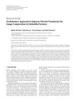
Fig. 1. Static and dynamic saliency maps: (a) Input video frame, (b) Static saliency map M
s

and (c) Dynamic saliency map M
d.
.

4. Face an important feature
Faces are one of the most important visual cues for communication. A lot of research has
examined the complex issue of face perception (Kanwisher & Yovel, 2006; Thorpe, 2002;

Palermo & Rhodes, 2007; Tsao & Livingstone, 2008; Goto & Tobimatsu, 2005), for a complete
review see (Dekowska et al., 2008). In this research, we just wanted to test whether faces
were gazed at during free viewing of dynamic scenes. Hence, to test if a face is an important
feature in the prediction of human eye movements, we hand-labelled the frames of the
videos used in the experiment described in section 2 with the position and the size of faces.
We manually created a face saliency map by adding a two dimensional Gaussian to the top
of each marked face: we called this saliency map the “true” face saliency map (Fig. 3). We
call “face” any kind of face (frontal or profile) as long as the face is big enough for the eyes
(at least one) and the mouth to be distinguished. Because it takes times to hand label all the
frames and because we wanted to test the influence of faces we only used a small part of the
whole database and we chose frames with at least one face (472 frames). Then, we computed
the mean NSS over these 472 frames between the human eye position density maps and the
different saliency model: the static saliency map, the dynamic saliency map and the “true”
face saliency map (Fig. 2). As noted above a saliency map is a good predictor of human eye
fixations if the corresponding NSS value is positive and high.




Recent Advances in Signal Processing198

filter corresponds to an intermediate map, m
ij
, which is the equivalent of an elementary
feature of Treisman's Theory (Treisman & Gelade, 1980).

3.2 The static pathway
The static pathway is dedicated to the extraction of the static features of the visual stimulus.
This pathway corresponds to the ventral pathway of the human visual system and processes
detailed visual information. It starts with the parvocellular output of the retina and is then,

processed by the bank of Gabor filters. Two types of interactions between filter outputs were
implemented: short interactions reinforce objects belonging to a specific orientation and
long interactions allow contour facilitation.
After the interactions and after being normalized between [0,1], each map m
ij
was multiplied
by
2
(max( ) )
ij ij
m m
where max(m
ij
) is the maximum value and
ij
m
is the average of the
elementary feature map m
ij
(Itti et al., 1998). Then, for each map, values smaller than 20% of
the maximum value max(m
ij
) were set to 0. Finally, the intermediate maps were added
together to obtain a static saliency map M
s
(x,y,k) for each frame k (Fig. 1).

3.3 The dynamic pathway
The dynamic pathway, which is equivalent to the dorsal pathway of the human visual
system, is fast and carries global information. Because we assumed that human gaze is

attracted by motion contrast (the motion of a region against the background), we applied a
background motion compensation (2D motion estimation, Odobez & Bouthemy, 1995)
before the retina process. This allowed us to estimate the relative motion of regions against
the background. The compensated frames were filtered by the retina model described above
to form the “Magnocellular-like” output. Because this output only contains low spatial
frequencies, its information would be processed by the Gabor filters with the three lowest
frequency bands. For each frame, the classical optical flow constraint was applied to the
Gabor filter outputs in the same frequency band. The solution of this flow constraint defined
a motion vector per pixel of a frame. Then we computed for each pixel the motion vector
module, corresponding to the speed, and its angle, corresponding to the motion direction.
Hence, the motion saliency of a region is proportional to its speed against the background.
Then, a temporal median filter was applied to remove possible noise (if a pixel had a motion
in one frame but not in the previous ones). The filter was applied to five successive frames
(the current frame and the four previous ones) and it was reinitialised after each shot cut. A
dynamic saliency map M
d
(x,y,k) was obtained for each frame k (Fig. 1).



Fig. 1. Static and dynamic saliency maps: (a) Input video frame, (b) Static saliency map M
s

and (c) Dynamic saliency map M
d.
.

4. Face an important feature
Faces are one of the most important visual cues for communication. A lot of research has
examined the complex issue of face perception (Kanwisher & Yovel, 2006; Thorpe, 2002;

Palermo & Rhodes, 2007; Tsao & Livingstone, 2008; Goto & Tobimatsu, 2005), for a complete
review see (Dekowska et al., 2008). In this research, we just wanted to test whether faces
were gazed at during free viewing of dynamic scenes. Hence, to test if a face is an important
feature in the prediction of human eye movements, we hand-labelled the frames of the
videos used in the experiment described in section 2 with the position and the size of faces.
We manually created a face saliency map by adding a two dimensional Gaussian to the top
of each marked face: we called this saliency map the “true” face saliency map (Fig. 3). We
call “face” any kind of face (frontal or profile) as long as the face is big enough for the eyes
(at least one) and the mouth to be distinguished. Because it takes times to hand label all the
frames and because we wanted to test the influence of faces we only used a small part of the
whole database and we chose frames with at least one face (472 frames). Then, we computed
the mean NSS over these 472 frames between the human eye position density maps and the
different saliency model: the static saliency map, the dynamic saliency map and the “true”
face saliency map (Fig. 2). As noted above a saliency map is a good predictor of human eye
fixations if the corresponding NSS value is positive and high.




Gaze prediction improvement by adding a face feature to a saliency model 199


Fig. 2. Mean NSS values for the different saliency map: the static M
s
, the dynamic M
d
and
the “true” face saliency map M
f
.

As we can see on figure 2 the mean NSS value for the true face saliency map is higher than
for the mean NSS for the static and the dynamic saliency maps (F(2,1413)=1009.81; p#0). The
large difference is due to the fact that we only study frames with at least one face.

Fig. 3. Examples of the “true” face saliency maps obtained with the hand-labelled faces: (a)
and (d) Input video frames, (b) and (e) Corresponding “true” face saliency maps M
f
, (c) and
(f) Superposition of the input frame and the “true” face saliency map.

We experimentally found that faces attract human gazes and hence computing saliency
models that highlight faces improves the predictions of a more traditional saliency model
considerably. We still want to answer different questions. Is a face on its own inside a scene
more or less salient than a face with other faces? Is a large face more salient than a small
one? To answer these questions we chose some clips according to the number of faces and
according to the size of faces.



4.1 Impact of the number of faces
To see the influence of the number of faces, we split the database according to the number of
faces inside the frames: three clip-snippets (121 frames) with only one face and three others
(134 frames) with more than one face. We computed the NSS value for each frame using the
“true” face saliency map and the subject’s eye position density maps. Figure 4 presents the
mean NSS value for the frames with only one face and for the frames with more than one
face. A high NSS value means a good correspondence between human eye position density
maps and “true” face saliency maps.

Fig. 4. Mean NSS values for the “true” face saliency maps compared with human eye

positions as a function of the number of faces in frames: for frames with strictly one face
(121) and for frames with more than one faces (134).

The NSS value is higher when there is only one face than when there are more than one face
(F(1,253) =52.25; p#0). There is a better correspondence between the saliency map and eye
positions. This could be predicted by the fact that if there is only one face, all the subjects
would gaze at this single face whereas if there are several faces on the same frame some
subjects would gaze at a particular face and other subjects would gaze at another face.
Hence, a frame with only one face is more salient than a frame with more than one face, in
the sense that it is easier to predict subjects’ eye positions. To take this result into account,
we chose to compute the face saliency map using an inversely proportional coefficient to the
number of faces. That means that if there is only one face on a frame the corresponding
saliency map would have higher values than the saliency map of a frame with more than
one face.
An example of the eye position on a frame with three faces is presented in figure 5. Subjects’
gazes are more spread out over the frame with three faces than over the frames with only
one face.

Recent Advances in Signal Processing200


Fig. 2. Mean NSS values for the different saliency map: the static M
s
, the dynamic M
d
and
the “true” face saliency map M
f
.

As we can see on figure 2 the mean NSS value for the true face saliency map is higher than
for the mean NSS for the static and the dynamic saliency maps (F(2,1413)=1009.81; p#0). The
large difference is due to the fact that we only study frames with at least one face.

Fig. 3. Examples of the “true” face saliency maps obtained with the hand-labelled faces: (a)
and (d) Input video frames, (b) and (e) Corresponding “true” face saliency maps M
f
, (c) and
(f) Superposition of the input frame and the “true” face saliency map.

We experimentally found that faces attract human gazes and hence computing saliency
models that highlight faces improves the predictions of a more traditional saliency model
considerably. We still want to answer different questions. Is a face on its own inside a scene
more or less salient than a face with other faces? Is a large face more salient than a small
one? To answer these questions we chose some clips according to the number of faces and
according to the size of faces.



4.1 Impact of the number of faces
To see the influence of the number of faces, we split the database according to the number of
faces inside the frames: three clip-snippets (121 frames) with only one face and three others
(134 frames) with more than one face. We computed the NSS value for each frame using the
“true” face saliency map and the subject’s eye position density maps. Figure 4 presents the
mean NSS value for the frames with only one face and for the frames with more than one
face. A high NSS value means a good correspondence between human eye position density
maps and “true” face saliency maps.

Fig. 4. Mean NSS values for the “true” face saliency maps compared with human eye
positions as a function of the number of faces in frames: for frames with strictly one face

(121) and for frames with more than one faces (134).

The NSS value is higher when there is only one face than when there are more than one face
(F(1,253) =52.25; p#0). There is a better correspondence between the saliency map and eye
positions. This could be predicted by the fact that if there is only one face, all the subjects
would gaze at this single face whereas if there are several faces on the same frame some
subjects would gaze at a particular face and other subjects would gaze at another face.
Hence, a frame with only one face is more salient than a frame with more than one face, in
the sense that it is easier to predict subjects’ eye positions. To take this result into account,
we chose to compute the face saliency map using an inversely proportional coefficient to the
number of faces. That means that if there is only one face on a frame the corresponding
saliency map would have higher values than the saliency map of a frame with more than
one face.
An example of the eye position on a frame with three faces is presented in figure 5. Subjects’
gazes are more spread out over the frame with three faces than over the frames with only
one face.

Gaze prediction improvement by adding a face feature to a saliency model 201


Fig. 5. Examples of eye positions on a frame with three faces: (a) Input video frame, (b)
Superimposition of the input frame and the “true” face saliency map and (c) Eye positions of
the fifteen subjects.

As we can see in figure 5 (c) subjects gazed at the different faces. To test how much subjects
gazed at different positions in a frames we computed a criterion to measure the dispersion
of eye positions between subjects using the equation (2):
2
,
2

,
1
i j
i j i
D
d
N




(2)
where N is the number of subjects and d
i,j
is the distance between the eye positions of
subjects i and j. Table 1 presents the mean dispersion value for frames with strictly one face
and for frames with more than one face.

Number of faces Strictly one More than one
Mean dispersion
1 252.3 7 279.9
Table 1. Mean dispersion values of eye positions between subjects on frames as a function of
the number of faces: strictly one and more than one.

As expected, the dispersion is significantly higher for frames with more than one face, than
for frames with only one face (F(1,253)=269.7; p#0). This is consistent with a higher NSS for
frames with only one face than more than one.

4.2 Impact of face size
The previous observations are made for faces with almost the same size (See Fig. 5). But

what happen if there is one big face and two small ones? It is difficult to understand exactly
how size influences eye movements as many configurations can occur: for example, if there
are two faces, one may be large and the other may be small, or the two faces may be large or
small, one may be in the foreground etc. Hence it is difficult to understand exactly what
happens for eye movements. Let us consider clips with only one face. These clips are then
split according to the size of the face: three clip snippets with only one small face (141
frames), three with a medium face (107 frames) and three with a large face (90 frames). The
diameter of the small face is around 30 pixels, the diameter of the medium face is around 50
pixels and the diameter of the large face is around 80 pixels. The mean NSS value was
computed for the frames with a small, a medium and a large face (Fig. 6).


Fig. 6. Mean NSS value for “true” face saliency maps compared with human eye positions
for frames of nine clip snippets as a function of face size.

Large faces give significantly lower results than small or medium faces (F(1,336)=18.25;
p=0.00002). The difference between small and medium faces is not significant (F(1,246)=0.04;
p=0.84). This could be expected in fact: when a face is small, all subjects will gaze at the
same position, that is, the small face, and if the face is large, then some subjects will gaze at
the eyes, other will gaze at the mouth etc. To verify this, we computed the mean dispersion
of subject eye positions for the frames with small, medium or large faces in Table 2.

Face size Small Medium Large
Mean dispersion
2 927.6 1 418.4 904.24
Table 2. Mean dispersion values of eye positions between subjects on frames as a function of
face size.

The dispersion of eye positions is significantly higher for small faces (F(2,335)=28.44; p#0).
The dispersion of eye positions for frames with medium faces is not significantly different

from the frames with large faces (F(1,195)=2.89; p=0.09). These results are apparently in
contradiction with the mean NSS values found. Hence, two main questions arise: (1) why do
frames with one small face lead to a higher dispersion than frames with a larger face? And
(2) why do frames that lead to more spread out eye positions give a higher NSS?
Most of the time, when a small face is on a frame it is because the character is filmed in a
wide view; the frame shows the whole character and the scene behind him which may be
complex. If the character moves his hand, or if there is something interesting in the
foreground, some subjects will tend to gaze at the moving or the interesting thing after
viewing the face of the character. On the other hand, if a large face is on a frame, this
corresponds to a close-up view of the character being filmed. Hence, there is little
information outside the character ‘s face and hence, subjects will tend to keep their focus on
the only interesting area: the face, and access in more detail the different parts of the face.
A small face could lead to a high dispersion value if some subjects gaze at other areas after
having gazed at the face, and a large face could lead to a low dispersion value as subject
gazes tend to be spread over the face area. This is illustrated in figure 7, where eye positions
were shown for a large face and for a small one. In this example a subject gazed at the
device at the bottom of the frame, increasing the dispersion of eye positions. This is why we
observed a high dispersion value of eye positions even for frames with a high NSS value
(example of frames with a small face). A small face with few eye positions outside of the
Recent Advances in Signal Processing202


Fig. 5. Examples of eye positions on a frame with three faces: (a) Input video frame, (b)
Superimposition of the input frame and the “true” face saliency map and (c) Eye positions of
the fifteen subjects.

As we can see in figure 5 (c) subjects gazed at the different faces. To test how much subjects
gazed at different positions in a frames we computed a criterion to measure the dispersion
of eye positions between subjects using the equation (2):
2

,
2
,
1
i j
i j i
D
d
N




(2)
where N is the number of subjects and d
i,j
is the distance between the eye positions of
subjects i and j. Table 1 presents the mean dispersion value for frames with strictly one face
and for frames with more than one face.

Number of faces Strictly one More than one
Mean dispersion
1 252.3 7 279.9
Table 1. Mean dispersion values of eye positions between subjects on frames as a function of
the number of faces: strictly one and more than one.

As expected, the dispersion is significantly higher for frames with more than one face, than
for frames with only one face (F(1,253)=269.7; p#0). This is consistent with a higher NSS for
frames with only one face than more than one.

4.2 Impact of face size
The previous observations are made for faces with almost the same size (See Fig. 5). But
what happen if there is one big face and two small ones? It is difficult to understand exactly
how size influences eye movements as many configurations can occur: for example, if there
are two faces, one may be large and the other may be small, or the two faces may be large or
small, one may be in the foreground etc. Hence it is difficult to understand exactly what
happens for eye movements. Let us consider clips with only one face. These clips are then
split according to the size of the face: three clip snippets with only one small face (141
frames), three with a medium face (107 frames) and three with a large face (90 frames). The
diameter of the small face is around 30 pixels, the diameter of the medium face is around 50
pixels and the diameter of the large face is around 80 pixels. The mean NSS value was
computed for the frames with a small, a medium and a large face (Fig. 6).


Fig. 6. Mean NSS value for “true” face saliency maps compared with human eye positions
for frames of nine clip snippets as a function of face size.

Large faces give significantly lower results than small or medium faces (F(1,336)=18.25;
p=0.00002). The difference between small and medium faces is not significant (F(1,246)=0.04;
p=0.84). This could be expected in fact: when a face is small, all subjects will gaze at the
same position, that is, the small face, and if the face is large, then some subjects will gaze at
the eyes, other will gaze at the mouth etc. To verify this, we computed the mean dispersion
of subject eye positions for the frames with small, medium or large faces in Table 2.

Face size Small Medium Large
Mean dispersion
2 927.6 1 418.4 904.24
Table 2. Mean dispersion values of eye positions between subjects on frames as a function of
face size.

The dispersion of eye positions is significantly higher for small faces (F(2,335)=28.44; p#0).
The dispersion of eye positions for frames with medium faces is not significantly different
from the frames with large faces (F(1,195)=2.89; p=0.09). These results are apparently in
contradiction with the mean NSS values found. Hence, two main questions arise: (1) why do
frames with one small face lead to a higher dispersion than frames with a larger face? And
(2) why do frames that lead to more spread out eye positions give a higher NSS?
Most of the time, when a small face is on a frame it is because the character is filmed in a
wide view; the frame shows the whole character and the scene behind him which may be
complex. If the character moves his hand, or if there is something interesting in the
foreground, some subjects will tend to gaze at the moving or the interesting thing after
viewing the face of the character. On the other hand, if a large face is on a frame, this
corresponds to a close-up view of the character being filmed. Hence, there is little
information outside the character ‘s face and hence, subjects will tend to keep their focus on
the only interesting area: the face, and access in more detail the different parts of the face.
A small face could lead to a high dispersion value if some subjects gaze at other areas after
having gazed at the face, and a large face could lead to a low dispersion value as subject
gazes tend to be spread over the face area. This is illustrated in figure 7, where eye positions
were shown for a large face and for a small one. In this example a subject gazed at the
device at the bottom of the frame, increasing the dispersion of eye positions. This is why we
observed a high dispersion value of eye positions even for frames with a high NSS value
(example of frames with a small face). A small face with few eye positions outside of the
Gaze prediction improvement by adding a face feature to a saliency model 203

face, will lead to a high dispersion, but can thus have a higher NSS than a large face with
more eye positions on the face, so lower dispersion. Hence, the NSS tends to reward
fixations that are less due to chance more strongly: as the salient region for a small face is
small, the eye positions that are in this region will be more strongly rewarded than the ones
on a larger face.

Fig. 7. Examples of eye positions on frames with a face of different sizes: (a) and (d) Input

video frames, (b) and (e) Superimposition of the input frame and the face saliency map and
(c) and (f) Eye positions of the fifteen subjects corresponding to the input frame
.

Considering the case of only one face, face size influences eye positions. If more than one
face is present, too many configurations can occur, and so, it is much more difficult to
generalize the size effect. That is why for this study, the size information was not integrated
to build the face saliency map from the face detector output.

5. Face detection algorithms
Various methods have been proposed to detect faces in images (Yang et al., 2002). We tested
three algorithms available on the web: the one proposed by Viola
2
and Jones (Viola & Jones,
2004), the one proposed by Rowley
3
(Rowley et al., 1998) and the one proposed by Nilsson
4

(Nilsson et al., 2007) which is called the Split-up SNoW face detector. In our study, the
stimuli are different from classical databases used to evaluate algorithm performance for
face detection. We chose stimuli which were very different from one to another, and most
faces are presented with various and textured backgrounds. The different algorithms were


2
Viola & Jones -
3
Rowley -
4

Nilsson -
objectId=13701&objectType=FILE

compared on one of the twenty clips presented to subjects (Table 3). This clip was hand-
labelled: 429 faces were marked.

Algorithms
Number of correct
detections
Number of false
positives
Viola & Jones, 2004
146 (34%) 77
Rowley et al., 1998
87 (20.3%) 25
Nilsson et al., 2007
Split-up SNoW
5

97 (22.6%) 6
Table 3. Three face detection algorithms: number of correct detections (also called true
positives) and false positives for one clip (745 frames with 429 faces present).

Because the videos chosen are different from traditional stimuli used to evaluate face
detection algorithm, the three algorithms detected less than half the faces. During the
snippets, characters are moving, can turn to profile view, can sometimes be occluded or can
have tilted faces. Faces can also be blurred as the characters move fast. All these cases
complicate the task of the face detection algorithms. The Viola and Jones algorithm has the
highest correct detection rate but also the highest false positive rate. Most of the time, false
positives are on textured regions. Because we wanted to create a face saliency map that

emphasizes only areas with a face, and we wanted to prevent the highlighting of false
positives, we chose to use the split-up SNoW face detector which has the lowest false
positive rate.

5.1 The split-up SNoW face detector
SNoW (Sparse Network of Winnows) is a learning architecture framework designed to learn
a large number of features. It can be used for a more general purpose as a multi-class
classifier. SNoW has been used successfully in several applications in the natural language
and visual processing domains.
If a face is detected, the algorithm returns the position and the size of a squared bounding
box containing the face detected. The algorithm detects faces with frontal views, even
partially occluded faces (i.e. faces with glasses) and slightly tilted faces, but it cannot
retrieve faces which are too occluded or profile views. We tested the efficiency of the SNoW
face detector algorithm on the whole database (14155 frames). As it takes time and it is
fastidious to hand-label all the faces for all the frames, we counted the number of frames
that contained at least one face and we found 6623 frames. The split-up SNoW face detector
gave 1566 frames with at least a correct detection and only 147 false positives. As already
said, the number of correct detections is quite low but, what is more important for our
purpose is that the number of false positive is very low. Hence, using this face detection
algorithm ensures that we will only emphasize areas with a very high probability of
containing a face. Examples of results for the split-up SNoW face detector are given in figure
8.


5
Results are given setting the parameter sens to 9 in the Matlab program.
Recent Advances in Signal Processing204

face, will lead to a high dispersion, but can thus have a higher NSS than a large face with
more eye positions on the face, so lower dispersion. Hence, the NSS tends to reward

fixations that are less due to chance more strongly: as the salient region for a small face is
small, the eye positions that are in this region will be more strongly rewarded than the ones
on a larger face.

Fig. 7. Examples of eye positions on frames with a face of different sizes: (a) and (d) Input
video frames, (b) and (e) Superimposition of the input frame and the face saliency map and
(c) and (f) Eye positions of the fifteen subjects corresponding to the input frame
.

Considering the case of only one face, face size influences eye positions. If more than one
face is present, too many configurations can occur, and so, it is much more difficult to
generalize the size effect. That is why for this study, the size information was not integrated
to build the face saliency map from the face detector output.

5. Face detection algorithms
Various methods have been proposed to detect faces in images (Yang et al., 2002). We tested
three algorithms available on the web: the one proposed by Viola
2
and Jones (Viola & Jones,
2004), the one proposed by Rowley
3
(Rowley et al., 1998) and the one proposed by Nilsson
4

(Nilsson et al., 2007) which is called the Split-up SNoW face detector. In our study, the
stimuli are different from classical databases used to evaluate algorithm performance for
face detection. We chose stimuli which were very different from one to another, and most
faces are presented with various and textured backgrounds. The different algorithms were

2

Viola & Jones -
3
Rowley -
4
Nilsson -
objectId=13701&objectType=FILE

compared on one of the twenty clips presented to subjects (Table 3). This clip was hand-
labelled: 429 faces were marked.

Algorithms
Number of correct
detections
Number of false
positives
Viola & Jones, 2004
146 (34%) 77
Rowley et al., 1998
87 (20.3%) 25
Nilsson et al., 2007
Split-up SNoW
5

97 (22.6%) 6
Table 3. Three face detection algorithms: number of correct detections (also called true
positives) and false positives for one clip (745 frames with 429 faces present).

Because the videos chosen are different from traditional stimuli used to evaluate face
detection algorithm, the three algorithms detected less than half the faces. During the
snippets, characters are moving, can turn to profile view, can sometimes be occluded or can

have tilted faces. Faces can also be blurred as the characters move fast. All these cases
complicate the task of the face detection algorithms. The Viola and Jones algorithm has the
highest correct detection rate but also the highest false positive rate. Most of the time, false
positives are on textured regions. Because we wanted to create a face saliency map that
emphasizes only areas with a face, and we wanted to prevent the highlighting of false
positives, we chose to use the split-up SNoW face detector which has the lowest false
positive rate.

5.1 The split-up SNoW face detector
SNoW (Sparse Network of Winnows) is a learning architecture framework designed to learn
a large number of features. It can be used for a more general purpose as a multi-class
classifier. SNoW has been used successfully in several applications in the natural language
and visual processing domains.
If a face is detected, the algorithm returns the position and the size of a squared bounding
box containing the face detected. The algorithm detects faces with frontal views, even
partially occluded faces (i.e. faces with glasses) and slightly tilted faces, but it cannot
retrieve faces which are too occluded or profile views. We tested the efficiency of the SNoW
face detector algorithm on the whole database (14155 frames). As it takes time and it is
fastidious to hand-label all the faces for all the frames, we counted the number of frames
that contained at least one face and we found 6623 frames. The split-up SNoW face detector
gave 1566 frames with at least a correct detection and only 147 false positives. As already
said, the number of correct detections is quite low but, what is more important for our
purpose is that the number of false positive is very low. Hence, using this face detection
algorithm ensures that we will only emphasize areas with a very high probability of
containing a face. Examples of results for the split-up SNoW face detector are given in figure
8.



5

Results are given setting the parameter sens to 9 in the Matlab program.
Gaze prediction improvement by adding a face feature to a saliency model 205


Fig. 8. Examples of correct detections (true positives) (marked with a white box) and missed
detections (false negatives) for the split-up SNoW face detector.

6. Saliency model: The face pathway
The face detection algorithm output needs to be converted into a saliency map. The
algorithm returns the position and the size of a squared bounding box containing the face
detected. How can this information be translated into a face saliency map? The face detector
gives a binary result: A pixel is equal to 1 if it is part of a face (the corresponding bounding
box) and 0 otherwise. In the few papers that dealt with face saliency maps, the bounding
boxes used to mark the face detected are replaced by a two-dimensional Gaussian. This
induced the centre of a face to be more salient than its border. For example, in (Cerf et al.,
2007) the “face conspicuity map” is normalized to a fixed range, in (Ma et al., 2005) the face
saliency map values are weighted by the position of the face, enhancing faces in the centre of
the frame.
As the final aim of our model is to provide a master saliency map by computing the fusion
of the three saliency maps, face M
f
, static M
s
and dynamic M
d
, the face saliency map was
normalized to give values in the same range as static and dynamic saliency map values. As
stated above, the face saliency map is intrinsically different from the static and the dynamic
saliency maps. On one hand, the face detection algorithm returns binary information:
presence or absence of face. On the other hand, static or dynamic saliency maps are

weighted “by nature”: more or less textured for the static saliency map and more or less
rapid for moving areas of the dynamic saliency map. The face saliency map was built by
replacing the bounding box of the algorithm output by a two-dimensional Gaussian. To be
in the same range as the static and the dynamic saliency maps, the maximum value of the
two-dimensional Gaussian was set to 5. Moreover, as stated above, a frame with only one
face is more salient than a frame with more than one face. To lessen the face saliency map
when more than one face is detected, the maximum of the Gaussian (after been multiplied
by five) was divided by N
1/3
where N is the number of faces detected on the frame. To sum
up, the Gaussian that replaced the bounding box that marked a detected face was set to
1/3
5
N
. We used the cube root of N to attenuate the effect of a high N value.

7. Evaluation
7.1. Fusions
Static, dynamic and face saliency maps do not have the same appearance. On one hand, the
static saliency map exhibits a large number of salient areas, corresponding to textured areas
that are spread over the whole image. On the other hand, the dynamic saliency map can
exhibit only small and compact areas corresponding to moving objects. Finally, the face
saliency map can be null when no face is detected.
A previous study detailed the analysis of the static and the dynamic pathways (Marat et al.,
2009). This study showed that a frame with a high maximum static saliency map value is
more salient than a frame with a lower maximum static saliency map value. Moreover, a
frame with high skewness of the dynamic saliency map is more salient than a frame with a
lower skewness value of the dynamic saliency map. A high skewness value corresponds to a
frame with only one compact moving area. To add the static saliency map multiplied by its
maximum to the dynamic saliency map multiplied by its skewness creating the master

saliency map provides better eye movement prediction than a simple sum. The face saliency
map was designed to reduce the maximum saliency value with the number of faces
detected. Hence, this maximum is characteristic for the face pathway. The fusion proposed
considers the particular features of each saliency map by weighting the raw saliency maps
by their relevant parameters (maximum or skewness) and provides better results. The
weighted saliency maps are defined as:
'
max( )


s
s s
M
M M

(3)
'
( )
d d d
M
skewness M M



(4)
'
max( )


f

f f
M
M M

(5)

To study the importance of the face pathway, we computed two different master saliency
maps: one using only the static and the dynamic maps (6) and another using the three maps
(7).
' '
s
d s d
M
M M



(6)
' ' '
s
df s d f
M
M M M

 

(7)

Note that if the face saliency map is null for a frame the master saliency map would depend
only on the static and the dynamic saliency maps. Moreover, to strengthen regions that are

salient in two different maps (static and dynamic, static and face or dynamic and face), a
more elaborate fusion, called “reinforced” fusion (M
Rsdf
), was proposed (8):
' ' ' ' ' ' ' ' 'Rsdf s d f s d s f d f
M
M M M M M M M M M        

(8)
This fusion reinforces the weighted fusion M
sdf
by adding multiplicative terms. We chose
multiplicative terms with only two maps because if we chose a multiplicative term with the
three maps when the face saliency map is null the multiplicative term would be null. If the
face saliency map is null the “reinforced” fusion takes advantage of the static and the
dynamic maps. In that case, the face saliency map does not improve the result but it does
not penalize the result either. Examples of these fusions integrating the face pathway are
proposed in figure 9. In figure 9 (a), the face on the right of the frame is moving, whereas the
Recent Advances in Signal Processing206


Fig. 8. Examples of correct detections (true positives) (marked with a white box) and missed
detections (false negatives) for the split-up SNoW face detector.

6. Saliency model: The face pathway
The face detection algorithm output needs to be converted into a saliency map. The
algorithm returns the position and the size of a squared bounding box containing the face
detected. How can this information be translated into a face saliency map? The face detector
gives a binary result: A pixel is equal to 1 if it is part of a face (the corresponding bounding
box) and 0 otherwise. In the few papers that dealt with face saliency maps, the bounding

boxes used to mark the face detected are replaced by a two-dimensional Gaussian. This
induced the centre of a face to be more salient than its border. For example, in (Cerf et al.,
2007) the “face conspicuity map” is normalized to a fixed range, in (Ma et al., 2005) the face
saliency map values are weighted by the position of the face, enhancing faces in the centre of
the frame.
As the final aim of our model is to provide a master saliency map by computing the fusion
of the three saliency maps, face M
f
, static M
s
and dynamic M
d
, the face saliency map was
normalized to give values in the same range as static and dynamic saliency map values. As
stated above, the face saliency map is intrinsically different from the static and the dynamic
saliency maps. On one hand, the face detection algorithm returns binary information:
presence or absence of face. On the other hand, static or dynamic saliency maps are
weighted “by nature”: more or less textured for the static saliency map and more or less
rapid for moving areas of the dynamic saliency map. The face saliency map was built by
replacing the bounding box of the algorithm output by a two-dimensional Gaussian. To be
in the same range as the static and the dynamic saliency maps, the maximum value of the
two-dimensional Gaussian was set to 5. Moreover, as stated above, a frame with only one
face is more salient than a frame with more than one face. To lessen the face saliency map
when more than one face is detected, the maximum of the Gaussian (after been multiplied
by five) was divided by N
1/3
where N is the number of faces detected on the frame. To sum
up, the Gaussian that replaced the bounding box that marked a detected face was set to
1/3
5

N
. We used the cube root of N to attenuate the effect of a high N value.

7. Evaluation
7.1. Fusions
Static, dynamic and face saliency maps do not have the same appearance. On one hand, the
static saliency map exhibits a large number of salient areas, corresponding to textured areas
that are spread over the whole image. On the other hand, the dynamic saliency map can
exhibit only small and compact areas corresponding to moving objects. Finally, the face
saliency map can be null when no face is detected.
A previous study detailed the analysis of the static and the dynamic pathways (Marat et al.,
2009). This study showed that a frame with a high maximum static saliency map value is
more salient than a frame with a lower maximum static saliency map value. Moreover, a
frame with high skewness of the dynamic saliency map is more salient than a frame with a
lower skewness value of the dynamic saliency map. A high skewness value corresponds to a
frame with only one compact moving area. To add the static saliency map multiplied by its
maximum to the dynamic saliency map multiplied by its skewness creating the master
saliency map provides better eye movement prediction than a simple sum. The face saliency
map was designed to reduce the maximum saliency value with the number of faces
detected. Hence, this maximum is characteristic for the face pathway. The fusion proposed
considers the particular features of each saliency map by weighting the raw saliency maps
by their relevant parameters (maximum or skewness) and provides better results. The
weighted saliency maps are defined as:
'
max( ) 
s
s s
M
M M

(3)
'
( )
d d d
M
skewness M M 

(4)
'
max( ) 
f
f f
M
M M

(5)

To study the importance of the face pathway, we computed two different master saliency
maps: one using only the static and the dynamic maps (6) and another using the three maps
(7).
' '
s
d s d
M
M M 

(6)
' ' '
s
df s d f

M
M M M  

(7)

Note that if the face saliency map is null for a frame the master saliency map would depend
only on the static and the dynamic saliency maps. Moreover, to strengthen regions that are
salient in two different maps (static and dynamic, static and face or dynamic and face), a
more elaborate fusion, called “reinforced” fusion (M
Rsdf
), was proposed (8):
' ' ' ' ' ' ' ' 'Rsdf s d f s d s f d f
M
M M M M M M M M M        

(8)
This fusion reinforces the weighted fusion M
sdf
by adding multiplicative terms. We chose
multiplicative terms with only two maps because if we chose a multiplicative term with the
three maps when the face saliency map is null the multiplicative term would be null. If the
face saliency map is null the “reinforced” fusion takes advantage of the static and the
dynamic maps. In that case, the face saliency map does not improve the result but it does
not penalize the result either. Examples of these fusions integrating the face pathway are
proposed in figure 9. In figure 9 (a), the face on the right of the frame is moving, whereas the
Gaze prediction improvement by adding a face feature to a saliency model 207

two faces on the left are not moving. In figure 9 (b) the three faces are almost equally salient,
but in figure 9 (c) the multiplicative reinforcement terms increase the saliency of the moving
face on the right of the frame.

Fig. 9. Example of master saliency maps: (a) Input video frame, (b) Corresponding master
saliency map computed using a weighted fusion of the three pathways M
sdf
, (c)
Corresponding master saliency map using the “reinforced” fusion of the three pathways
M
Rsdf.

7.2. Evaluation of different saliency maps
The first evaluation was done on the database of “true” face saliency maps which were
hand-labelled. Each saliency map was weighted as explained in section 6.1. The results are
presented in Table 4.

Saliency maps M
s
M
d
M
f
M
sd
M
sdf
M
Rsdf
Mean NSS
0.68 0.84 4.46 1.00 3.38 3.99
Standard deviation
0.72 1.03 2.19 0.80 1.63 2.05

Table 4. Evaluation of the different saliency map and the fusion, on the database where a
“true” face saliency map was hand-labelled.

As stated above, the face saliency map gives better results than the static or the dynamic
ones (F(2,1413)=1009.81; p#0). The fusion which did not take face saliency maps into account
gives a lower result than the fusions with face saliency maps (F(2,1413)=472.33; p#0), and
the reinforced fusion is even better than a more classical fusion (F(1,942)=25.63; p=4.98x10
-7
).
Subsequently, the NSS was computed for each frame of the whole database (14155 frames)
using the different model saliency maps and the eye movement data. The face saliency map
is obtained using the split-up SNoW face detector and the weighting and fusion previously
explained. In order to test the contribution of face pathway, the mean NSS value was
calculated using the saliency map given by each pathway independently and the different
possible fusions. The mean NSS value is plotted for six models of saliency maps (M
s
, M
d
, M
f
,
M
sd
, M
sdf
, M
Rsdf
) in comparison with human data in figure 10. The NSS values are given for
the saliency maps (M
s

, M
d
and M
f
) but note that the NSS results would be the same for the
weighted saliency maps (M
s’
, M
d’
and M
f’
), as multiplying the saliency map by a constant
did not change the NSS value.


Fig. 10. Mean NSS values on the whole database (14155 frames) for six models of saliency
maps (static, dynamic, face, weighted fusion of the static and dynamic pathways M
sd
,
weighted fusion of the static, the dynamic and the face pathway M
sdf
and a “reinforced”
weighted fusion M
Rsdf
).

As presented in (Marat et al., 2009), the dynamic saliency maps are more predictive than the
static ones. The fusion of the static and the dynamic saliency maps improves the prediction
of the model: the static and the dynamic information needs to be considered to improve the
model prediction. The results of the face pathway should not be considered; in fact, it gives

the lowest results but only because a small number of frames contain at least one face
detected compared to the total number of frames (12% of the whole database).The weighted
fusion integrating the face pathway (M
sdf
) is significantly better than the weighted fusion of
the static and the saliency maps (M
sd
), (F(1,28308)=255.39; p#0). Integrating the face
pathway increases the model prediction; hence, as already observed, faces are crucial
information to predict eye positions. The “reinforced” fusion integrating multiplicative
terms (M
Rsdf
), increasing saliency in regions that are salient in two maps, gives the best
results, outperforming the previous fusion (M
sdf
), (F(1,28308)=25.91; p=3.6x10
-9
). The
contribution of the face pathway in attracting our gaze is undeniable. The face pathway
improves the results greatly, faces have to be integrated into a saliency model to make the
results of the model match the experimental results more closely.

8. Conclusion
When viewing scenes, faces are almost immediately gazed on. This was shown in static
images (Cerf et al., 2007). We report in this research the same phenomenon using dynamic
stimuli. This means that even if there are moving objects, faces rapidly attracted gazes. To
study the influence of faces on gaze, we ran an experiment to record the eye movements of
subjects when looking freely at videos. We used videos with various contents, with or
without faces with textured backgrounds and with or without moving objects. This
experiment enabled us to check that faces are fixated on within the first milliseconds and

independently of the scenes (presence or not of moving objects etc.). Moreover, we showed
that a face is more salient if it is the only face on the frame. In order to take this into account,
we added a “face pathway” to a bottom-up saliency model inspired by the biology. The
“face pathway” uses the Split-up Snow face detector algorithm. Hence, the model splits the
visual signal into static, dynamic, and face saliency maps. The static saliency map
emphasizes orientation and spatial frequency contrasts. The dynamic saliency map
Recent Advances in Signal Processing208

two faces on the left are not moving. In figure 9 (b) the three faces are almost equally salient,
but in figure 9 (c) the multiplicative reinforcement terms increase the saliency of the moving
face on the right of the frame.

Fig. 9. Example of master saliency maps: (a) Input video frame, (b) Corresponding master
saliency map computed using a weighted fusion of the three pathways M
sdf
, (c)
Corresponding master saliency map using the “reinforced” fusion of the three pathways
M
Rsdf.

7.2. Evaluation of different saliency maps
The first evaluation was done on the database of “true” face saliency maps which were
hand-labelled. Each saliency map was weighted as explained in section 6.1. The results are
presented in Table 4.

Saliency maps M
s
M
d
M

f
M
sd
M
sdf
M
Rsdf
Mean NSS
0.68 0.84 4.46 1.00 3.38 3.99
Standard deviation
0.72 1.03 2.19 0.80 1.63 2.05
Table 4. Evaluation of the different saliency map and the fusion, on the database where a
“true” face saliency map was hand-labelled.

As stated above, the face saliency map gives better results than the static or the dynamic
ones (F(2,1413)=1009.81; p#0). The fusion which did not take face saliency maps into account
gives a lower result than the fusions with face saliency maps (F(2,1413)=472.33; p#0), and
the reinforced fusion is even better than a more classical fusion (F(1,942)=25.63; p=4.98x10
-7
).
Subsequently, the NSS was computed for each frame of the whole database (14155 frames)
using the different model saliency maps and the eye movement data. The face saliency map
is obtained using the split-up SNoW face detector and the weighting and fusion previously
explained. In order to test the contribution of face pathway, the mean NSS value was
calculated using the saliency map given by each pathway independently and the different
possible fusions. The mean NSS value is plotted for six models of saliency maps (M
s
, M
d
, M

f
,
M
sd
, M
sdf
, M
Rsdf
) in comparison with human data in figure 10. The NSS values are given for
the saliency maps (M
s
, M
d
and M
f
) but note that the NSS results would be the same for the
weighted saliency maps (M
s’
, M
d’
and M
f’
), as multiplying the saliency map by a constant
did not change the NSS value.


Fig. 10. Mean NSS values on the whole database (14155 frames) for six models of saliency
maps (static, dynamic, face, weighted fusion of the static and dynamic pathways M
sd
,

weighted fusion of the static, the dynamic and the face pathway M
sdf
and a “reinforced”
weighted fusion M
Rsdf
).

As presented in (Marat et al., 2009), the dynamic saliency maps are more predictive than the
static ones. The fusion of the static and the dynamic saliency maps improves the prediction
of the model: the static and the dynamic information needs to be considered to improve the
model prediction. The results of the face pathway should not be considered; in fact, it gives
the lowest results but only because a small number of frames contain at least one face
detected compared to the total number of frames (12% of the whole database).The weighted
fusion integrating the face pathway (M
sdf
) is significantly better than the weighted fusion of
the static and the saliency maps (M
sd
), (F(1,28308)=255.39; p#0). Integrating the face
pathway increases the model prediction; hence, as already observed, faces are crucial
information to predict eye positions. The “reinforced” fusion integrating multiplicative
terms (M
Rsdf
), increasing saliency in regions that are salient in two maps, gives the best
results, outperforming the previous fusion (M
sdf
), (F(1,28308)=25.91; p=3.6x10
-9
). The
contribution of the face pathway in attracting our gaze is undeniable. The face pathway

improves the results greatly, faces have to be integrated into a saliency model to make the
results of the model match the experimental results more closely.

8. Conclusion
When viewing scenes, faces are almost immediately gazed on. This was shown in static
images (Cerf et al., 2007). We report in this research the same phenomenon using dynamic
stimuli. This means that even if there are moving objects, faces rapidly attracted gazes. To
study the influence of faces on gaze, we ran an experiment to record the eye movements of
subjects when looking freely at videos. We used videos with various contents, with or
without faces with textured backgrounds and with or without moving objects. This
experiment enabled us to check that faces are fixated on within the first milliseconds and
independently of the scenes (presence or not of moving objects etc.). Moreover, we showed
that a face is more salient if it is the only face on the frame. In order to take this into account,
we added a “face pathway” to a bottom-up saliency model inspired by the biology. The
“face pathway” uses the Split-up Snow face detector algorithm. Hence, the model splits the
visual signal into static, dynamic, and face saliency maps. The static saliency map
emphasizes orientation and spatial frequency contrasts. The dynamic saliency map
Gaze prediction improvement by adding a face feature to a saliency model 209

emphasizes motion contrasts and the face saliency map emphasizes faces proportionally to
the number of faces. Then, these three maps are originally fuzzed by taking into account the
specificity of each saliency map. The fusion showed that the “face pathway” significantly
increases the predictions of the model.

9. References
Carmi R. & Itti L. (2006). Visual causes versus correlates of attentional selection in dynamic
scenes. Vision Research, Vol. 46, No. 26, pp. 4333-4345
Cerf M.; Harel J.; Einhäuser W. & Koch C. (2007). Predicting gaze using low-level saliency
combined with face detection, in Proceedings of Neural Information System NIPS 2007
Dekowska M.; Kuniecki M. & Jaskowski P. (2008). Facing facts: neuronal mechanisms of face

perception. Acta Neurobiologiae Experimentalis, Vol. 68, No. 2, pp. 229-252
Goto Y. & Tobimatsu S. (2005). An electrophysiological study of the initial step of face
perception. International Congress Series, Vol. 1278, pp. 45-48
Itti L.; Koch C. & Niebur E. (1998). A model of saliency-based visual attention for rapid
scene analysis. IEEE Trans. on PAMI, Vol. 20, No. 11, pp. 1254-1259
Kanwisher N. & Yovel G. (2006). The fusiform face area: a cortical region specialized for the
perception of faces. Philosophical transactions of the royal society Biological sciences,
Vol. 361, No. 1476, pp. 2109-2128
Le Meur O.; Le Callet P. & Barba D. (2006). A coherent computational approach to model
bottom-up visual attention. IEEE Trans. on PAMI, Vol. 28, No. 5, pp. 802-817
Marat S.; Ho Phuoc T.; Granjon L.; Guyader N.; Pellerin D. & Dugué-Guérin A. (2009).
Modelling spatio-temporal saliency to predict gaze direction for short videos.
International Journal of Computer Vision, Vol. 82, No. 3, pp. 231-243
Marat S.; Ho Phuoc T.; Granjon L.; Guyader N.; Pellerin D. & Dugué-Guérin A. (2008).
Spatio-temporal saliency model to predict eye movements in video free viewing, in
Proceedings of Eusipco 2008, Lausanne, Switzerland
Odobez J M. & Bouthemy P. (1995). Robust multiresolution estimation of parametric
motion models. Journal of visual communication and image representation, Vol. 6, pp.
348-365
Palermo R. & Rhodes G. (2007). Are you always on my mind? A review of how face
perception and attention interact. Neuropsychologia, Vol. 45, No. 1, pp. 75-92
Peters R. J. & Itti L. (2008). Applying computational tools to predict gaze direction in
interactive visual environments. ACM Trans. On Applied Perception, Vol. 5, No. 2
Thorpe S. J. (2002). Ultra-rapid scene categorization with a wave of spikes, in Proceedings of
the Second International Workshop on Biologically Motivated Computer Vision, Vol. 2525,
pp. 1-15
Treisman A. M. & Gelade G. (1980). A feature-integration theory of attention. Cognitive
Psychology, Vol. 12, No. 1, pp. 97-136
Tsao D. Y. & Livingstone M. S. (2008). Mechanisms of face perception. Annu. Rev. Neuroscci.,
Vol. 31, pp. 411-437

Viola P. & Jones M. J. (2004). Robust real time face detection. International Journal of Computer
Vision, Vol. 57, No. 2, pp. 137-154
Yang M H.; Kriegman D. J. & Ahuja N. (2002). Detecting faces in images: a survey. IEEE
Trans. on PAMI, Vol. 24, No. 1, pp. 34-58
Recent Advances in Signal Processing210
Suppression of Correlated Noise 211
Suppression of Correlated Noise
Jan Aelterman, Bart Goossens, Aleksandra Pizurica and Wilfried Philips
X

Suppression of Correlated Noise

Jan Aelterman, Bart Goossens, Aleksandra Pizurica and Wilfried Philips
Ghent University, TELIN-IPI-IBBT
Belgium

1. Introduction

Many signal processing applications involve noise suppression (colloquially known as
denoising). In this chapter we will focus on image denoising. There is a substantial amount
of literature on this topic. We will start by a short overview:
Many algorithms denoise data by using some transformation on the data, thereby
considering the signal (the image) as a linear combination of a number of atoms. For
denoising purposes, it is beneficial to use such transformations, where the noise-free image
can be accurately represented by only a limited number of these atoms. This property is
sometimes referred to as sparsity. The aim in denoising is to detect which of these atoms
represent significant signal energy from the large amount of possible atoms representing
noise.
A lot of research has been performed to find representations that are as sparse as possible
for ‘natural’ images. Examples of such representations are the Fourier basis, the Discrete

Wavelet Transform (DWT) (Donoho, 1995), the Curvelet Transform (Starck, 2002), the
Shearlet transform (Easley, 2006), the dual-tree complex wavelet transform (Kingsbury,
2001; Selesnick, 2005), … Many denoising techniques designed for one such representation
can be used in others, because the principles (exploiting sparsity) are the same. Without
exception, these denoising methods try to preserve the small amount of significant
transform coefficients, i.e the ones carrying the information, while suppressing the large
amount of transform coefficients that only represent noise. The sparsity property of natural
images (in its proper transform domain) ensures that there will be only a very small amount
of significant transform coefficients, which allows to suppress a large amount of the noise
energy in the insignificant transform coefficients. Multiresolution denoising techniques
range from rudimentary approaches such as hard or soft thresholding of coefficients
(Donoho, 1995) to more advanced approaches that try to capture some statistical
significance behind atom coefficients by imposing appropriate prior models (Malfait, 1997;
Romberg, 2001; Portilla, 2003; Pizurica, 2006; Guerrero-Colon, 2008; Goossens, 2009;).
Another class of algorithms try to exploit image (self-) similarity. It has been noted that
many images have repetitive features on the level of pixel blocks. This was exploited in
recent literature through the use of statistical averaging schemes of similar blocks (Buades
2005; Buades, 2008; Goossens, 2008) or grouping of similar blocks and 3d transform domain
denoising (Dabov, 2007).
13
Recent Advances in Signal Processing212

In practice, processes that corrupt data can often not be described using a simple additive
white gaussian noise (AWGN) model. Many of these processes can be modelled as linear
filtering process of a white Gaussian noise source, which results into correlated noise. Some
correlated noise generating processes are described in section 2. The majority of the
mentioned denoising techniques are only designed for white noise and relatively few
techniques have been reported that are capable of suppressing correlated noise. In this
chapter, we present some techniques for noise estimation in section 4 and image modelling
in section 3, which form the theoretical basis for the (correlated) noise removal techniques

explained in section 5. Section 6 contains demonstration denoising experiments, using the
explained denoising algorithms, and presents a conclusion.

2. Sources of Correlated Noise
2.1 From white noise to correlated noise
In this section, the aim is to find a proper description of correlated noise. Once established,
we will use it to describe several correlated noise processes in the remainder of this section.
Since the spatial correlation is of interest, rather than time/spatially-varying noise statistics,
we will assume stationarity throughout this chapter. Stationarity means that the
autocorrelation function only depends on the relative displacement between two pixels,
rather than their absolute positions. This is evident from (1), a random process generating
samples f(n) is called white if it has zero mean and a delta function as autocorrelation
function r
f
(n):


)(])()([)(
0)(
nmnfmfEnr
nfE
f




(1)

The Wiener–Khinchin theorem states that the power spectral density (PSD) of a (wide-sense
stationary) random signal f(n) is the Fourier transform of the corresponding autocorrelation

function r(n):





n
nj
enrR


)()(


(2)

This means that for white noise, the PSD is equal to a constant value, hence the name white
(white light has a flat spectrum). When a linear filter h(n), with Discrete Time Fourier
Transform (DTFT) H(ω) is applied (often inadvertently) to the white noise random signal,
the resulting effect on the autocorrelation function and PSD of
)()()(' nhnfnf 

is:
 
2
)()()('
)()(])(')('[)('

HHHR
mnhmhmnfmfEnr

m









(3)

This result shows that the correlated noise PSD R’(ω) is the squared magnitude response of
the linear filter DTFT, hence one can think of correlated noise as white noise subjected to
linear filtering. In analogy with the term ‘white noise’ this is sometimes referred to as
‘colored noise’. In the following sections, some real world technologies will be explained
from the perspective of noise correlation.

2.2 Phase Alternating Line (PAL) Television
PAL is a transmission standard used in colour analogue broadcast television systems.
Dating back to the 1950s, there are several bandwidth saving techniques that are very nice in
their own right, but are responsible for the noise in PAL television. One is the deinterlacing
mechanism (Kwon, 2003). Another is the use of a different modulation and filtering
schemes. We will restrict us here to show the PSD of a patch of noise from a PAL signal
broadcast:

Fig. 1. noisy PAL broadcast of a sports event and PSD of noise in a green color channel of
the PAL broadcast.

It is clear that the noise here is almost cut off horizontally, leading to stripe like artifacts and

there is significant energy in the lower vertical frequencies, leading to vertical streaks. It is
therefore naive to assume noise in PAL/NTSC television to be white.

2.3 Demosaicing
Modern digital cameras use a rectangular arrangement of photosensitive elements. This
matrix arrangement allows the interleaving of photosensitive elements of different color
sensitivity. This interleaving allows sampling of full color images without the use of three
matrices of photosensitive elements. One very popular arrangement is the Bayer pattern
(Bayer, 1976), shown in figure 2.

Fig. 2. Bayer mosaic pattern of photosensitive elements in a camera sensor

There exist a wide range of techniques for reconstructing the full color image from mosaiced
image data. A thorough study of these techniques is beyond the scope of this chapter.
Instead, we compare the simplest approach with one state of the art technique, from the
viewpoint of noise correlation.
Suppression of Correlated Noise 213

In practice, processes that corrupt data can often not be described using a simple additive
white gaussian noise (AWGN) model. Many of these processes can be modelled as linear
filtering process of a white Gaussian noise source, which results into correlated noise. Some
correlated noise generating processes are described in section 2. The majority of the
mentioned denoising techniques are only designed for white noise and relatively few
techniques have been reported that are capable of suppressing correlated noise. In this
chapter, we present some techniques for noise estimation in section 4 and image modelling
in section 3, which form the theoretical basis for the (correlated) noise removal techniques
explained in section 5. Section 6 contains demonstration denoising experiments, using the
explained denoising algorithms, and presents a conclusion.

2. Sources of Correlated Noise

2.1 From white noise to correlated noise
In this section, the aim is to find a proper description of correlated noise. Once established,
we will use it to describe several correlated noise processes in the remainder of this section.
Since the spatial correlation is of interest, rather than time/spatially-varying noise statistics,
we will assume stationarity throughout this chapter. Stationarity means that the
autocorrelation function only depends on the relative displacement between two pixels,
rather than their absolute positions. This is evident from (1), a random process generating
samples f(n) is called white if it has zero mean and a delta function as autocorrelation
function r
f
(n):


)(])()([)(
0)(
nmnfmfEnr
nfE
f




(1)

The Wiener–Khinchin theorem states that the power spectral density (PSD) of a (wide-sense
stationary) random signal f(n) is the Fourier transform of the corresponding autocorrelation
function r(n):






n
nj
enrR


)()(


(2)

This means that for white noise, the PSD is equal to a constant value, hence the name white
(white light has a flat spectrum). When a linear filter h(n), with Discrete Time Fourier
Transform (DTFT) H(ω) is applied (often inadvertently) to the white noise random signal,
the resulting effect on the autocorrelation function and PSD of
)()()(' nhnfnf 

is:
 
2
)()()('
)()(])(')('[)('

HHHR
mnhmhmnfmfEnr
m










(3)

This result shows that the correlated noise PSD R’(ω) is the squared magnitude response of
the linear filter DTFT, hence one can think of correlated noise as white noise subjected to
linear filtering. In analogy with the term ‘white noise’ this is sometimes referred to as
‘colored noise’. In the following sections, some real world technologies will be explained
from the perspective of noise correlation.

2.2 Phase Alternating Line (PAL) Television
PAL is a transmission standard used in colour analogue broadcast television systems.
Dating back to the 1950s, there are several bandwidth saving techniques that are very nice in
their own right, but are responsible for the noise in PAL television. One is the deinterlacing
mechanism (Kwon, 2003). Another is the use of a different modulation and filtering
schemes. We will restrict us here to show the PSD of a patch of noise from a PAL signal
broadcast:

Fig. 1. noisy PAL broadcast of a sports event and PSD of noise in a green color channel of
the PAL broadcast.

It is clear that the noise here is almost cut off horizontally, leading to stripe like artifacts and
there is significant energy in the lower vertical frequencies, leading to vertical streaks. It is
therefore naive to assume noise in PAL/NTSC television to be white.

2.3 Demosaicing

Modern digital cameras use a rectangular arrangement of photosensitive elements. This
matrix arrangement allows the interleaving of photosensitive elements of different color
sensitivity. This interleaving allows sampling of full color images without the use of three
matrices of photosensitive elements. One very popular arrangement is the Bayer pattern
(Bayer, 1976), shown in figure 2.

Fig. 2. Bayer mosaic pattern of photosensitive elements in a camera sensor

There exist a wide range of techniques for reconstructing the full color image from mosaiced
image data. A thorough study of these techniques is beyond the scope of this chapter.
Instead, we compare the simplest approach with one state of the art technique, from the
viewpoint of noise correlation.
Recent Advances in Signal Processing214

Since all of these techniques perform interpolation in some way, we are confident that the
conclusion will be similar for all demosaicing techniques. When using patches of white
noise as input data for an image mosaic sensor, the PSD of the demosaicing noise is shown
in figure (3)-(4). Because white noise is used as input for a demosaicing system, the
reconstruction will be a color image of correlated noise. Since we are assuming additive
noise, this will be a good model for type of noise that is encountered in color digital camera
images. In figure (3), we compared the simplest demosaicing approach, bilinear
demosaicing, for both the green and the red color plane. Since the red data is subsampled
more, the demosaicing treats both color planes differently, explaining the difference in PSD
bandwidth. Figure (4) shows the result using a state-of-the-art demosaicing technique
(Aelterman, 2009). There is no visible difference between the green and blue plane PSD here,
because the algorithm works in a luminance/chrominance approximation rather than
red/green/blue space.

Fig. 3. PSD of the green channel (left) and a red/blue channel(right) from the demosaiced
white noise patch using bilinear demosaicing.

Fig. 4. PSD of the green channel (left) and a red/blue channel(right) from the demosaiced
white noise patch using the technique described in (Aelterman, 2009)

The demosaicing experiments in figure 4 and 5 also show that the low pass part of the PSD
is brighter, meaning it represents more noise energy. This is explained through the tendency

of demosaicing algorithms to favour smooth color patches, as this is an accurate model for
natural images.

Fig. 5. The full color lighthouse image (left) corrupted with white noise (middle) and with
correlated noise due to bilinear demosaicing (right)

2.3 Thermal Camera’s
Many thermal cameras are based on the push broom or whisk broom principle. Only very
few infrared sensors are used, which have to be reused through an optics system in order to
scan the different pixels positions, creating the complete image. This raster scan principle is
illustrated in figure 6.

Fig. 6. Example of a raster scanned image pattern (whisk broom imaging)

The downside of such imaging principles is that they sometimes exhibit streaking noise
artifacts, which can be attributed to the sensor and sampling circuitry. Since pixel intensities
at different spatial positions are acquired using the same sensor, temporal correlation in the
noisy sensor data results in spatial noise correlation in the acquired image. For thermal
cameras, noise can be approximated using a 1/f frequency dependency of the noise (Borel,
1996). This type of ‘pink’ noise is very common in electronic devices and becomes apparent
when reusing image sensors for different pixels in the image at high sample rates.
Suppression of Correlated Noise 215

Since all of these techniques perform interpolation in some way, we are confident that the
conclusion will be similar for all demosaicing techniques. When using patches of white
noise as input data for an image mosaic sensor, the PSD of the demosaicing noise is shown
in figure (3)-(4). Because white noise is used as input for a demosaicing system, the
reconstruction will be a color image of correlated noise. Since we are assuming additive
noise, this will be a good model for type of noise that is encountered in color digital camera
images. In figure (3), we compared the simplest demosaicing approach, bilinear
demosaicing, for both the green and the red color plane. Since the red data is subsampled
more, the demosaicing treats both color planes differently, explaining the difference in PSD
bandwidth. Figure (4) shows the result using a state-of-the-art demosaicing technique
(Aelterman, 2009). There is no visible difference between the green and blue plane PSD here,
because the algorithm works in a luminance/chrominance approximation rather than
red/green/blue space.

Fig. 3. PSD of the green channel (left) and a red/blue channel(right) from the demosaiced
white noise patch using bilinear demosaicing.


Fig. 4. PSD of the green channel (left) and a red/blue channel(right) from the demosaiced
white noise patch using the technique described in (Aelterman, 2009)

The demosaicing experiments in figure 4 and 5 also show that the low pass part of the PSD
is brighter, meaning it represents more noise energy. This is explained through the tendency

of demosaicing algorithms to favour smooth color patches, as this is an accurate model for
natural images.

Fig. 5. The full color lighthouse image (left) corrupted with white noise (middle) and with
correlated noise due to bilinear demosaicing (right)

2.3 Thermal Camera’s
Many thermal cameras are based on the push broom or whisk broom principle. Only very
few infrared sensors are used, which have to be reused through an optics system in order to
scan the different pixels positions, creating the complete image. This raster scan principle is
illustrated in figure 6.

Fig. 6. Example of a raster scanned image pattern (whisk broom imaging)

The downside of such imaging principles is that they sometimes exhibit streaking noise
artifacts, which can be attributed to the sensor and sampling circuitry. Since pixel intensities
at different spatial positions are acquired using the same sensor, temporal correlation in the
noisy sensor data results in spatial noise correlation in the acquired image. For thermal
cameras, noise can be approximated using a 1/f frequency dependency of the noise (Borel,
1996). This type of ‘pink’ noise is very common in electronic devices and becomes apparent
when reusing image sensors for different pixels in the image at high sample rates.
Recent Advances in Signal Processing216


Fig. 7. PSD of ‘pink noise’, an approximate model of noise in some types of electronic
devices through time

Pink noise can easily be simulated, by filtering a time sequence of white pseudorandom
numbers with a 1/f filter characteristic and then adding those noise samples to the signal
values in a raster scan pattern. Figure 8 shows this type of noise on the Einstein image.

Fig. 8. The Einstein image with simulated whisk broom imaging 1/f noise.

The streaking noise artifacts are clearly visible.

2.4 Magnetic Resonance Imaging
Magnetic Resonance Imaging is a non-invasive imaging technique. The Signal to Noise ratio
(SNR) is heavily dependent on scan time. Longer scans are not only less comfortable for the
patient, it is also less economical for the scanner operator and it increases the chance of
involuntary patient movement. Because MRI technology acquires a Fourier transformed
version of the image, rather than the image itself, patient movement during a scan translates

to ‘echo’-like artifacts in the image, which is much more detrimental to the diagnostic image
quality than simple blurring in conventional photography.
These facts are a major motivation for scanner manufacturers, who have created a wide
range of tricks and technologies that allow an MRI scan to be made faster or less susceptible
to motion artifacts. Noise in MRI is traditionally considered white (e.g. Nowak, 1999;
Pizurica, 2003), and this is indeed a good noise model for theoretical MRI, but in practice,
almost all clinical MRI acquisition devices use one or more acceleration techniques. As an
illustration we now explain a few:
In K-space subsampling, bands of the spectrum of the signal are simply not scanned.
Elliptical filtering is similar, where only elliptical area around the K-space center is sampled.
An illustration and example of this principe is shown in figure 9.

Fig. 9. (left) PSD of K-space subsampled and elliptically filtered noise (right) Brain MRI with
simulated K-space subsampled and elliptically filtered MRI noise

It is clearly visible that for this situation, the noise creates stripe-like artifacts rather than
being statistically independent from one pixel to another.

3. Describing natural images

3.1 Sparsity
When generating an image using purely random generators, chances are it will look like
random noise. To the authors’ knowledge, nobody ever succeeded in generating an image

this way that looks like a ‘natural’ picture, which could have come from a camera. This is
because what people consider ‘natural’ images is a very small subset of all possible images.
Natural images have specific properties. These properties have been the object of intensive
study throughout the years and are of interest here, as it is what will enable the statistical
separation of noise from signal in images.
An easily verifiable, intuitive, property of natural images is that they are smoothly varying
signals, which give low frequency responses, delineated by lines (edges). This is somewhat
quantified by the inverse power scaling law, natural image PSD’s are inversely proportional
in magnitude to the squared modulus of the spatial frequency variable (Ruderman, 1994;
Field, 1987):
Suppression of Correlated Noise 217


Fig. 7. PSD of ‘pink noise’, an approximate model of noise in some types of electronic
devices through time

Pink noise can easily be simulated, by filtering a time sequence of white pseudorandom
numbers with a 1/f filter characteristic and then adding those noise samples to the signal
values in a raster scan pattern. Figure 8 shows this type of noise on the Einstein image.

Fig. 8. The Einstein image with simulated whisk broom imaging 1/f noise.

The streaking noise artifacts are clearly visible.

2.4 Magnetic Resonance Imaging
Magnetic Resonance Imaging is a non-invasive imaging technique. The Signal to Noise ratio
(SNR) is heavily dependent on scan time. Longer scans are not only less comfortable for the
patient, it is also less economical for the scanner operator and it increases the chance of
involuntary patient movement. Because MRI technology acquires a Fourier transformed
version of the image, rather than the image itself, patient movement during a scan translates

to ‘echo’-like artifacts in the image, which is much more detrimental to the diagnostic image
quality than simple blurring in conventional photography.
These facts are a major motivation for scanner manufacturers, who have created a wide
range of tricks and technologies that allow an MRI scan to be made faster or less susceptible
to motion artifacts. Noise in MRI is traditionally considered white (e.g. Nowak, 1999;
Pizurica, 2003), and this is indeed a good noise model for theoretical MRI, but in practice,
almost all clinical MRI acquisition devices use one or more acceleration techniques. As an
illustration we now explain a few:
In K-space subsampling, bands of the spectrum of the signal are simply not scanned.
Elliptical filtering is similar, where only elliptical area around the K-space center is sampled.
An illustration and example of this principe is shown in figure 9.

Fig. 9. (left) PSD of K-space subsampled and elliptically filtered noise (right) Brain MRI with
simulated K-space subsampled and elliptically filtered MRI noise

It is clearly visible that for this situation, the noise creates stripe-like artifacts rather than
being statistically independent from one pixel to another.

3. Describing natural images

3.1 Sparsity
When generating an image using purely random generators, chances are it will look like
random noise. To the authors’ knowledge, nobody ever succeeded in generating an image
this way that looks like a ‘natural’ picture, which could have come from a camera. This is
because what people consider ‘natural’ images is a very small subset of all possible images.
Natural images have specific properties. These properties have been the object of intensive
study throughout the years and are of interest here, as it is what will enable the statistical
separation of noise from signal in images.
An easily verifiable, intuitive, property of natural images is that they are smoothly varying

signals, which give low frequency responses, delineated by lines (edges). This is somewhat
quantified by the inverse power scaling law, natural image PSD’s are inversely proportional
in magnitude to the squared modulus of the spatial frequency variable (Ruderman, 1994;
Field, 1987):
Recent Advances in Signal Processing218






2
1
)('R


(4)

Where η is a small number (|η|<1). This observation, coupled with the mathematical
elegance of the Gaussian distribution, motivated early image processing engineers to model
both image and noise as Gaussian distributed, in some transform domain. The Minimization
of the Mean Squared Error Bayesian risk estimator (MMSE) denoising solution is the well
known Wiener filter. However, the Gaussian distribution does not account for the relatively
large number of outliers when considering e.g. wavelet filter responses. In fact, as a
consequence of thinking of images as smooth regions delineated by edges, most coefficients
will be far smaller than predicted by the Gaussian model and a small number will be really
big.

Fig. 10. Comparison of a Gaussian distribution (full line) with a more heavily tailed
distribution, which is a better model for the transform coefficient distribution of natural

images

This property, sometimes referred to as sparsity, is better modeled by a more heavily tailed
distribution model, a comparison between both types of prior distributions is shown in
figure 11. The next section gives some examples.

3.2 Marginal statistics of multiresolution image transformation coefficients
It is clearly visible in multiresolution decompositions that marginals distributions of
coefficients exhibit highly non Gaussian behaviour. In fact, more leptokurtic distributions
account better for the heavy tailed marginal distributions that one encounters in practice.
For this reason, other distributions, such as the Laplacian (also known as the exponential
power distribution) or Generalized Laplacian (Mallat, 1989; Pizurica, 2006) have been
applied in more effective techniques. The Generalized Laplacian distribution is described in
(5), with λ and υ called the scale and shape parameter and Γ() the gamma function.

















 exp
1
2
)(p


(5)


The Gaussian Scale Mixtures (GSM) (Wainwright, 2000) is a more elegant alternative,
because it can be extended more easily to the multivariate situation, which is advantageous
when considering spatial noise correlation. A random vector β is a GSM when it can be
written as:
Uz
d




(6)

Where U is a Normally distributed random vector with mean 0 and covariance matrix C,
z>0 is a random scalar variable, independent of U and superscript d means ‘equal in
distribution’. The marginal distribution of β can then be written as:













 dz
z
C
z
Cz
p
t
N
2
exp)(
)2(
1
)(
1
21
2






(7)

Both the Generalized Laplacian and the GSM model are parameterized, which means that
some (often empirical) parameter estimation is required for the parameters. For the
Generalized Laplacian, this can be done by fitting the sample kurtosis and variance, while
for the GSM covariance matrix and hidden multiplier z distribution, there exist an
expectation maximization (EM) solution (Portilla, 2003). It is also possible to assume a fixed
distribution for the hidden multiplier z, which will enhance the kurtosis of the marginal
distribution p(β) in order to have a more heavily tailed distribution that corresponds more
to the model from section 3.1 e.g. Jeffey’s prior (p(z)=1/z).

3.2 Selfsimilarity
Another property of natural images is that they often contain a lot of redundant
information. Natural images contain a lot of repeating structures and texture. Often,
similarity can also be encountered at different scales. Some images of plants or art can be
surprisingly well described using fractals, meaning that they can be described as built up of
downscaled copies of themselves. This suggests that there is a lot of similarity in an image, a
property called selfsimilarity. Since noise is typically more spatially independent, it is a
good idea to find a description for self similarity, which can then be exploited in a denoising
algorithm. This is done by finding similar image patches for every pixel in the image.



Suppression of Correlated Noise 219






2
1

)('R


(4)

Where η is a small number (|η|<1). This observation, coupled with the mathematical
elegance of the Gaussian distribution, motivated early image processing engineers to model
both image and noise as Gaussian distributed, in some transform domain. The Minimization
of the Mean Squared Error Bayesian risk estimator (MMSE) denoising solution is the well
known Wiener filter. However, the Gaussian distribution does not account for the relatively
large number of outliers when considering e.g. wavelet filter responses. In fact, as a
consequence of thinking of images as smooth regions delineated by edges, most coefficients
will be far smaller than predicted by the Gaussian model and a small number will be really
big.

Fig. 10. Comparison of a Gaussian distribution (full line) with a more heavily tailed
distribution, which is a better model for the transform coefficient distribution of natural
images

This property, sometimes referred to as sparsity, is better modeled by a more heavily tailed
distribution model, a comparison between both types of prior distributions is shown in
figure 11. The next section gives some examples.

3.2 Marginal statistics of multiresolution image transformation coefficients
It is clearly visible in multiresolution decompositions that marginals distributions of
coefficients exhibit highly non Gaussian behaviour. In fact, more leptokurtic distributions
account better for the heavy tailed marginal distributions that one encounters in practice.
For this reason, other distributions, such as the Laplacian (also known as the exponential
power distribution) or Generalized Laplacian (Mallat, 1989; Pizurica, 2006) have been
applied in more effective techniques. The Generalized Laplacian distribution is described in

(5), with λ and υ called the scale and shape parameter and Γ() the gamma function.
















 exp
1
2
)(p


(5)


The Gaussian Scale Mixtures (GSM) (Wainwright, 2000) is a more elegant alternative,
because it can be extended more easily to the multivariate situation, which is advantageous
when considering spatial noise correlation. A random vector β is a GSM when it can be
written as:

Uz
d




(6)

Where U is a Normally distributed random vector with mean 0 and covariance matrix C,
z>0 is a random scalar variable, independent of U and superscript d means ‘equal in
distribution’. The marginal distribution of β can then be written as:












 dz
z
C
z
Cz
p
t

N
2
exp)(
)2(
1
)(
1
21
2






(7)

Both the Generalized Laplacian and the GSM model are parameterized, which means that
some (often empirical) parameter estimation is required for the parameters. For the
Generalized Laplacian, this can be done by fitting the sample kurtosis and variance, while
for the GSM covariance matrix and hidden multiplier z distribution, there exist an
expectation maximization (EM) solution (Portilla, 2003). It is also possible to assume a fixed
distribution for the hidden multiplier z, which will enhance the kurtosis of the marginal
distribution p(β) in order to have a more heavily tailed distribution that corresponds more
to the model from section 3.1 e.g. Jeffey’s prior (p(z)=1/z).

3.2 Selfsimilarity
Another property of natural images is that they often contain a lot of redundant
information. Natural images contain a lot of repeating structures and texture. Often,
similarity can also be encountered at different scales. Some images of plants or art can be

surprisingly well described using fractals, meaning that they can be described as built up of
downscaled copies of themselves. This suggests that there is a lot of similarity in an image, a
property called selfsimilarity. Since noise is typically more spatially independent, it is a
good idea to find a description for self similarity, which can then be exploited in a denoising
algorithm. This is done by finding similar image patches for every pixel in the image.



Recent Advances in Signal Processing220


Fig. 11. Several natural images (top), with a similarity map (MSE) for the cyan pixel
(bottom). Note how there is a large number of similar pixels for natural images.

Finding similar patches in an image can be done by block matching: For some neighborhood
window size L, the mean squared error is taken between every neighborhood in the image
and the neighborhood around the current pixel. Similar pixels exhibit a low MSE and the
selfsimilarity property ensures that there will be plenty of such similar patches in a natural
image. Figure 11 shows the similarity values for every pixel in the image, with respect to
the image indicated by the arrow for a neighborhood size of 3x3. Black means a high
similarity (low MSE). Note that for the cactus image, all the needles are found to be similar,
even though the perspective causes the needles on the top of the image to be smaller
versions of the needles at the bottom, which is an example of where similarity can be found
at different scales.

4. Estimating noise Correlation

4.1 Signal-free data
In many applications, noise can be considered additive. Additive noise means that even
after linear image transformations, the noise remains additive. In this case, the noise

statistics are not signal dependent, and could just as well be estimated from signal-free data.
In fact, this is easier, because the estimation will not be hindered by the signal. Many
applications allow for the acquisition of signal-free data. This is the case for MRI images,
where physical limitations ensure the existence of signal-free regions next to the scanned
subject in the MRI image. For an unknown thermal camera type, one could photograph a
surface of even temperature. Similar techniques can be used for optical photography and
many other imaging modalities. When presented with such signal-free, noisy data, the
autocorrelation function can be calculated in a straightforward way.

Since the Discrete Fourier Transform (DFT) can be used as a good approximation for the
Discrete Time Fourier Transform (DTFT) in (2) for finite data, it is possible to obtain the
autocorrelation function from the power spectral density, which can be estimated from the
finite noisy, signal-free input data f(n):

N
knj
ekFkFnr
enfkF
N
k
N
knj
N
n


2
1
0
2

1
0
)()()(
)()(













(8)

This way of using the DTFT to estimate the autocorrelation function of a stationary process
is computationally more efficient than calculating the autocorrelation function or covariance
matrix explicitly through e.g. convolution in the image domain.

4.3 Estimating correlated noise in transform domains
Calculating the pixel (voxel) autocorrelation function / covariance matrix is just part of the
solution. Since many denoising algorithms operate in a transform domain, it is necessary to
transform the autocorrelation function / covariance matrix as well. A transformed
covariance matrix enables the whitening of transform coefficients, which allows the use of a
white noise denoising algorithm.
One obvious way to obtain the transformed covariance matrices, is through Monte Carlo

simulations. First patches of noise are generated, then transformed into the transform
domain and then the noise covariance matrix are calculated for every obtained subband.
Doing this for multiresolution transforms with a lot of scales either results in heavy memory
requirements or high computational requirements, in order to get meaningful results.
In (Goossens, 2009), a different approach is presented. Many transformations can be viewed
as banks of linear filters. Applying a transform filter G(ω) to the signal f’(n) from (3), the
PSD R’’(ω) becomes:
)()(')()(''

GRGR 

(9)
When also taking the subsampling step from many shift-variant transformations (such as
the discrete wavelet transform) into account, the transform becomes less trivial:
 


''(2 ) ( ) '( ) ( ) '( ) ( ) '( ) ( ) '( )R G F G F G F G F

           
      

(10)

In (10) we see the appearance of crosscorrelation terms
)(')('

FF which seem to
indicate that it is not possible to simply filter the autocorrelation function such as in (9).
However, considering the stationarity assumption, the following should also hold:

 

)
(')()(')()(')()(')()2(''

 FGFGFGFGR
(11)

The minus sign is caused by a one sample shift prior to subsampling. Now the
crosscorrelation terms appear with an inverted sign with respect to (10). Since the
stationarity assumption implies equality between (11) en (10) it follows that the
crosscorrelation are zero. This means that the calculation of the transform autocorrelation
function simplifies to:
)()(')()()(')()2(''

 GRGGRGR


(12)

Suppression of Correlated Noise 221


Fig. 11. Several natural images (top), with a similarity map (MSE) for the cyan pixel
(bottom). Note how there is a large number of similar pixels for natural images.

Finding similar patches in an image can be done by block matching: For some neighborhood
window size L, the mean squared error is taken between every neighborhood in the image
and the neighborhood around the current pixel. Similar pixels exhibit a low MSE and the
selfsimilarity property ensures that there will be plenty of such similar patches in a natural

image. Figure 11 shows the similarity values for every pixel in the image, with respect to
the image indicated by the arrow for a neighborhood size of 3x3. Black means a high
similarity (low MSE). Note that for the cactus image, all the needles are found to be similar,
even though the perspective causes the needles on the top of the image to be smaller
versions of the needles at the bottom, which is an example of where similarity can be found
at different scales.

4. Estimating noise Correlation

4.1 Signal-free data
In many applications, noise can be considered additive. Additive noise means that even
after linear image transformations, the noise remains additive. In this case, the noise
statistics are not signal dependent, and could just as well be estimated from signal-free data.
In fact, this is easier, because the estimation will not be hindered by the signal. Many
applications allow for the acquisition of signal-free data. This is the case for MRI images,
where physical limitations ensure the existence of signal-free regions next to the scanned
subject in the MRI image. For an unknown thermal camera type, one could photograph a
surface of even temperature. Similar techniques can be used for optical photography and
many other imaging modalities. When presented with such signal-free, noisy data, the
autocorrelation function can be calculated in a straightforward way.

Since the Discrete Fourier Transform (DFT) can be used as a good approximation for the
Discrete Time Fourier Transform (DTFT) in (2) for finite data, it is possible to obtain the
autocorrelation function from the power spectral density, which can be estimated from the
finite noisy, signal-free input data f(n):

N
knj
ekFkFnr
enfkF

N
k
N
knj
N
n


2
1
0
2
1
0
)()()(
)()(













(8)

This way of using the DTFT to estimate the autocorrelation function of a stationary process
is computationally more efficient than calculating the autocorrelation function or covariance
matrix explicitly through e.g. convolution in the image domain.

4.3 Estimating correlated noise in transform domains
Calculating the pixel (voxel) autocorrelation function / covariance matrix is just part of the
solution. Since many denoising algorithms operate in a transform domain, it is necessary to
transform the autocorrelation function / covariance matrix as well. A transformed
covariance matrix enables the whitening of transform coefficients, which allows the use of a
white noise denoising algorithm.
One obvious way to obtain the transformed covariance matrices, is through Monte Carlo
simulations. First patches of noise are generated, then transformed into the transform
domain and then the noise covariance matrix are calculated for every obtained subband.
Doing this for multiresolution transforms with a lot of scales either results in heavy memory
requirements or high computational requirements, in order to get meaningful results.
In (Goossens, 2009), a different approach is presented. Many transformations can be viewed
as banks of linear filters. Applying a transform filter G(ω) to the signal f’(n) from (3), the
PSD R’’(ω) becomes:
)()(')()(''

GRGR 

(9)
When also taking the subsampling step from many shift-variant transformations (such as
the discrete wavelet transform) into account, the transform becomes less trivial:
 
 
''(2 ) ( ) '( ) ( ) '( ) ( ) '( ) ( ) '( )R G F G F G F G F


           
      

(10)

In (10) we see the appearance of crosscorrelation terms
)(')('

FF which seem to
indicate that it is not possible to simply filter the autocorrelation function such as in (9).
However, considering the stationarity assumption, the following should also hold:
 

)
(')()(')()(')()(')()2(''

 FGFGFGFGR
(11)

The minus sign is caused by a one sample shift prior to subsampling. Now the
crosscorrelation terms appear with an inverted sign with respect to (10). Since the
stationarity assumption implies equality between (11) en (10) it follows that the
crosscorrelation are zero. This means that the calculation of the transform autocorrelation
function simplifies to:
)()(')()()(')()2(''

 GRGGRGR


(12)