Recent Advances in Signal Processing 2011 Part 9 pptx

Detection of echo generated in mobile phones 267
Detection of echo generated in mobile phones
Tõnu Trump
X

Detection of echo generated in
mobile phones

Tõnu Trump
Ericsson AB
Sweden

1. Introduction

Echo is a phenomenon where part of the sound energy transmitted to a receiver reflects back
to the sender. In telephony it usually happens because of acoustic coupling between the
receiver’s loudspeaker and microphone or because of reflections of signals at the impedance
mismatches in the analogue parts of the telephony system. In mobile phones one has to deal
with acoustic echoes i.e. the signal played in the phones loudspeaker can be picked up by
microphone of the same mobile phone.
People are used to the echoes that surround us in everyday life due to e.g. reflections of our
speech from the walls of rooms where we are located. Those echoes arrive with a relatively
short delay (in the order of milliseconds) and are, as a rule, attenuated. In a modern
telephone system on the other hand the echoes may return with a delay that is not natural
for human beings. The main reason for delay is in those systems signal processing like
speech coding and interleaving. For example in a PSTN to GSM telephone call the one way
transmission delay is around 100 ms making the echo to return after 200 ms. Echo that
returns with this long delay is very unnatural to a human being and makes talking very
difficult. Therefore the echo needs to be removed.
Ideally the mobile terminals should handle their own echoes in such a way that no echo is
transmitted back to the telephony system. Even though many of the mobile phones

currently in use are able to handle their echoes properly, there are still models that do not.
ITU-T has recognized this problem and has recently consented the Recommendation G.160,
“Voice Enhancement Devices” that addresses these issues (ITU-T G.160). Following this
standard we concentrate on the scenario where the mobile echo control device is located in
the telephone system.
It should be noted that differently from the conventional network- or acoustic echo problem
(Sondhi & Berkley 1980; Signal Processing June 2006), where one normally assumes that the
echo is present, it is not given that any echo is returned from the mobile phone at all.
Therefore, the first step of a mobile echo removal algorithm should be detection of the
presence of the echo, as argued in (Perry 2007). A simple level based echo detector is also
proposed in (Perry 2007).
16
Recent Advances in Signal Processing268

Line Spectrum Pair (LSP) vectors, which are transformation of the linear prediction filter
coefficients that have better quantization properties. The fractional pitch lags that represent
the fundamental frequency of speech signal. The innovative codevectors that are used to
code the excitation signal. And finally there are the pitch and innovative gains. In the
detector, the LSP vectors are converted to the Linear Prediction (LP) filter coefficients and
interpolated to obtain LP filters at each subframe. Then, at each 40-sample subframe the
excitation is constructed by adding the adaptive and innovative codevectors scaled by their
respective gains and the speech is reconstructed by filtering the excitation through the LP
synthesis filter. Finally, the reconstructed speech signal is passed through an adaptive
postfilter.
The basic structure of the decoder in a simplified form but sufficient for our purposes is
shown in Figure 1 and described by the equation (1).
)(
)(
)(
1

1
1
d
n
T
p
c
zA
zA
zAzg
gc








(1)
In the above c denotes the innovative codevector, g
c
denotes the innovative gain (fixed
codebook gain), g
p
is the pitch gain, γ
n
and γ
d
are the postfilter constants and A(z) denotes

the LP synthesis filter. T is the fractional pitch lag, commonly referred to as “pitch period”
throughout this chapter.












Fig. 1. Simplified structure of AMR decoder

Of the parameters present in AMR coded bit-stream, the pitch period or the fundamental
frequency of the speech signal is believed to have the best chance to pass a nonlinear echo
path unaltered or with a little modification. An intuitive reason for this is that a nonlinear
system would likely generate harmonics but it would not alter the fundamental frequency
of a sine wave passing it. We therefore select the pitch period as the parameter of interest.
Fixed
code
book
Pitc
h

LP
syn-
thesis

Post
filtering

To design a mobile echo detector we first examine briefly the Adaptive Multi Rate (AMR)
codec (3GPP TS 26.090) in Section 2. In Section 3 we present our derivation of the detector,
which is followed by its performance analysis in Section 4. Some practicalities are explained
in Section 5. Section 6 summarizes our simulation study.
Following the terminology common in mobile telephony, we use the term downlink to
denote the transmission direction toward the mobile phone and the term uplink for the
direction toward the telephony system.

2. Problem formulation

In order to detect the echo, which is a (modified) reflection of the original signal one needs a
similarity measure between the downlink and the uplink signals. The echo path for the echo,
generated by the mobile handsets is nonlinear and non-stationary due to the speech codecs
and radio transmission in the echo path, which makes it difficult to use traditional linear
methods like adaptive filters, applied directly to the waveform of the signals. As argued in
(Perry 2007), the proper echo removal mechanism in this situation is a nonlinear processor,
similar to the one that is used after the linear echo cancellation in ordinary network echo
cancellers. In addition, as our measurements with various commercially available mobile
telephones show, a large part of popular phone models are equipped with proper means of
echo cancellation and do not produce any echo at all. Invoking a nonlinear processor based
echo removal in such calls can only harm the voice quality and should therefore be avoided.
That’s why the first step of any mobile echo reduction system that is placed in the telephone
system should be detection of the presence of echo. The nonlinear processor should then be
applied only if the presence of echo has first been established.
Another important point is that speech traverses in the mobile system in coded form and
that’s why it is advantageous, if our detector were able to work directly with coded speech
signals. Herein we therefore attempt to design a detector that uses the parameters present in

coded speech to detect the presence of echo and estimate its delay. Exact value of the delay
associated with the mobile echo is usually unknown and therefore needs to be estimated.
The total echo delay builds up of the delays of speech codecs, interleaving in radio interface
and other signal processing equipment that appear in the echo path together with unknown
transport delays and is typically in the order of couple of hundreds of milliseconds.
The problem addressed herein is that the simple level based echo detector is not always
reliable enough due to the impact of signals other than echo. The signals that are disturbing
for echo detection originate from the microphone of the mobile phone and are actually the
ones telephone system is supposed to carry to the other party of the telephone conversation.
This is usually referred to as double talk problem in the echo cancellation literature. In this
chapter we propose a detector that is not sensitive to double talk as shown in sequel of the
chapter.
Let us now examine the structure of the AMR speech codec that is the codec used in GSM
and UMTS mobile networks. The AMR codec switches between eight modes with different
bit-rates ranging from 4.75 kbit/s to 12.2 kbit/s to code the speech signal. According to
(3GPP TS 26.090), the AMR codec uses the following parameters to represent speech. The
Detection of echo generated in mobile phones 269

Line Spectrum Pair (LSP) vectors, which are transformation of the linear prediction filter
coefficients that have better quantization properties. The fractional pitch lags that represent
the fundamental frequency of speech signal. The innovative codevectors that are used to
code the excitation signal. And finally there are the pitch and innovative gains. In the
detector, the LSP vectors are converted to the Linear Prediction (LP) filter coefficients and
interpolated to obtain LP filters at each subframe. Then, at each 40-sample subframe the
excitation is constructed by adding the adaptive and innovative codevectors scaled by their
respective gains and the speech is reconstructed by filtering the excitation through the LP
synthesis filter. Finally, the reconstructed speech signal is passed through an adaptive
postfilter.
The basic structure of the decoder in a simplified form but sufficient for our purposes is
shown in Figure 1 and described by the equation (1).

)(
)(
)(
1
1
1
d
n
T
p
c
zA
zA
zAzg
gc








(1)
In the above c denotes the innovative codevector, g
c
denotes the innovative gain (fixed
codebook gain), g
p
is the pitch gain, γ

n
and γ
d
are the postfilter constants and A(z) denotes
the LP synthesis filter. T is the fractional pitch lag, commonly referred to as “pitch period”
throughout this chapter.












Fig. 1. Simplified structure of AMR decoder

Of the parameters present in AMR coded bit-stream, the pitch period or the fundamental
frequency of the speech signal is believed to have the best chance to pass a nonlinear echo
path unaltered or with a little modification. An intuitive reason for this is that a nonlinear
system would likely generate harmonics but it would not alter the fundamental frequency
of a sine wave passing it. We therefore select the pitch period as the parameter of interest.
Fixed
code
book
Pitc
h

LP
syn-
thesis
Post
filtering

To design a mobile echo detector we first examine briefly the Adaptive Multi Rate (AMR)
codec (3GPP TS 26.090) in Section 2. In Section 3 we present our derivation of the detector,
which is followed by its performance analysis in Section 4. Some practicalities are explained
in Section 5. Section 6 summarizes our simulation study.
Following the terminology common in mobile telephony, we use the term downlink to
denote the transmission direction toward the mobile phone and the term uplink for the
direction toward the telephony system.

2. Problem formulation

In order to detect the echo, which is a (modified) reflection of the original signal one needs a
similarity measure between the downlink and the uplink signals. The echo path for the echo,
generated by the mobile handsets is nonlinear and non-stationary due to the speech codecs
and radio transmission in the echo path, which makes it difficult to use traditional linear
methods like adaptive filters, applied directly to the waveform of the signals. As argued in
(Perry 2007), the proper echo removal mechanism in this situation is a nonlinear processor,
similar to the one that is used after the linear echo cancellation in ordinary network echo
cancellers. In addition, as our measurements with various commercially available mobile
telephones show, a large part of popular phone models are equipped with proper means of
echo cancellation and do not produce any echo at all. Invoking a nonlinear processor based
echo removal in such calls can only harm the voice quality and should therefore be avoided.
That’s why the first step of any mobile echo reduction system that is placed in the telephone
system should be detection of the presence of echo. The nonlinear processor should then be

applied only if the presence of echo has first been established.
Another important point is that speech traverses in the mobile system in coded form and
that’s why it is advantageous, if our detector were able to work directly with coded speech
signals. Herein we therefore attempt to design a detector that uses the parameters present in
coded speech to detect the presence of echo and estimate its delay. Exact value of the delay
associated with the mobile echo is usually unknown and therefore needs to be estimated.
The total echo delay builds up of the delays of speech codecs, interleaving in radio interface
and other signal processing equipment that appear in the echo path together with unknown
transport delays and is typically in the order of couple of hundreds of milliseconds.
The problem addressed herein is that the simple level based echo detector is not always
reliable enough due to the impact of signals other than echo. The signals that are disturbing
for echo detection originate from the microphone of the mobile phone and are actually the
ones telephone system is supposed to carry to the other party of the telephone conversation.
This is usually referred to as double talk problem in the echo cancellation literature. In this
chapter we propose a detector that is not sensitive to double talk as shown in sequel of the
chapter.
Let us now examine the structure of the AMR speech codec that is the codec used in GSM
and UMTS mobile networks. The AMR codec switches between eight modes with different
bit-rates ranging from 4.75 kbit/s to 12.2 kbit/s to code the speech signal. According to
(3GPP TS 26.090), the AMR codec uses the following parameters to represent speech. The
Recent Advances in Signal Processing270

 
   































otherwise. ,0
,
2
ln,min
exp
2

1
bwa
ab
tTtT
Hwp
dlul








(6)
Under the hypothesis H
0
, the distribution of w is assumed to be uniform within the interval
[a, b],
 








otherwise. ,0
,

1
0
bwa
ab
Hwp


(7)
We assume that the values taken by the random processes w(t) at various time instances are
statistically independent. Then the joint probability density is product of the individual
densities
 
 
 
 
 
 














N
t
N
t
HtwpHp
HtwpHp
1
00
1
11
.w
w



(8)
Let us now design a likelihood ratio test (Van Trees 1971) for the hypotheses mentioned
above. We assume that the cost for a correct decision is zero and the cost for any fault is one.
We also assume that both hypotheses have equal a priori probabilities. Then the test is given
by
 
   
,1
1
2
ln,min
exp
2
0
1

1
1
H
H
N
t
N
t
dlul
ul
ab
ab
tTtT
T








































(9)
Taking the logarithm and simplifying the above we obtain the following test
     
.ln
2
ln
2

ln,min
0
1
1



















abN
ab
tTtT
H
H
N
t

dlul







(10)
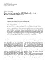
The decision device thus needs to compute the absolute distance between the uplink- and
downlink pitch periods for all delays, , of interest, saturate the absolute differences at
–σ ln[2σβ / (b - a)], sum up the results and compare the sum with a threshold. The structure
of the decision device is shown in Figure 2.



3. Derivation

In this section we derive a structure for the echo detector based on comparison of uplink
and downlink pitch periods. The derivation follows the principles of statistical hypothesis
testing theory described e.g. in (Van Trees 1971; Kay 1998).
Denote the uplink pitch period for the frame t as


tT
ul
and the downlink pitch period for
the frame t -  as





tT
dl
. The uplink pitch period will be treated as a random variable due
to the presence of pitch estimation errors and the contributions from the true signal from
mobile side.
Let us also denote the difference between uplink and downlink pitch periods as






 tTtTtw
dlul
,

(2)
Then we have the following two hypotheses:
H
0
: the echo is not present and the uplink pitch period is formed based only on the
signals present at the mobile side
H
1
: the uplink signal contains echo as indicated by the similarity of uplink and
downlink pitch periods
Under hypothesis H
1

, the process, w, models the errors of echo pitch estimation made
by the speech codec residing in mobile phone but also the contribution from signal entering
the microphone of the mobile phone. Our belief is that the distribution of the estimation
errors can be well approximated by the Laplace distribution and that the contribution from
the microphone signal gives a uniform floor to the distribution function. Some motivation
for selecting this particular model can be found in Section 6.1.
We thus assume that under the hypothesis H
1
the distribution function of w is given by
 
   



























otherwise. 0
,,exp
2
1
max
1
bwa
ab
tTtT
Hwp
dlul





(3)
The constant , in the above equation, is a design parameter that can be used to weight the
Laplace and uniform components and  is the parameter of Laplace distribution. The
variables a and b are determined by the limits in which the pitch period can be represented
in the AMR codec. In the 12.2 kbit/s mode the pitch period ranges from 18 to 143 and in the
other modes from 20 to 143. This gives us limits for the difference between uplink and
downlink pitch periods a = -125 and b = 125 in 12.2 kbit/s mode and a = -123, b = 123 in all

the other modes.  is a constant normalizing the probability density function so that it
integrates to unity. Solving
 
1

dwwp
b
a


(4)
for  we obtain
  
.
11
2
ln2 ab
ab
ab


















(5)
Equation (3) can be rewritten in a more convenient form for further derivation
Detection of echo generated in mobile phones 271

 
   































otherwise. ,0
,
2
ln,min
exp
2
1
bwa
ab
tTtT
Hwp
dlul






(6)
Under the hypothesis H
0
, the distribution of w is assumed to be uniform within the interval
[a, b],
 








otherwise. ,0
,
1
0
bwa
ab
Hwp


(7)
We assume that the values taken by the random processes w(t) at various time instances are
statistically independent. Then the joint probability density is product of the individual
densities
 

 
 
 
 
 













N
t
N
t
HtwpHp
HtwpHp
1
00
1
11
.w
w

(8)
Let us now design a likelihood ratio test (Van Trees 1971) for the hypotheses mentioned
above. We assume that the cost for a correct decision is zero and the cost for any fault is one.
We also assume that both hypotheses have equal a priori probabilities. Then the test is given
by
 
   
,1
1
2
ln,min
exp
2
0
1
1
1
H
H
N
t
N
t
dlul
ul
ab
ab

tTtT
T








































(9)
Taking the logarithm and simplifying the above we obtain the following test
     
.ln
2
ln
2
ln,min
0
1
1




















abN
ab
tTtT
H
H
N
t
dlul







(10)
The decision device thus needs to compute the absolute distance between the uplink- and
downlink pitch periods for all delays, , of interest, saturate the absolute differences at
–σ ln[2σβ / (b - a)], sum up the results and compare the sum with a threshold. The structure

of the decision device is shown in Figure 2.



3. Derivation

In this section we derive a structure for the echo detector based on comparison of uplink
and downlink pitch periods. The derivation follows the principles of statistical hypothesis
testing theory described e.g. in (Van Trees 1971; Kay 1998).
Denote the uplink pitch period for the frame t as


tT
ul
and the downlink pitch period for
the frame t -  as




tT
dl
. The uplink pitch period will be treated as a random variable due
to the presence of pitch estimation errors and the contributions from the true signal from
mobile side.
Let us also denote the difference between uplink and downlink pitch periods as












tTtTtw
dlul
,

(2)
Then we have the following two hypotheses:
H
0
: the echo is not present and the uplink pitch period is formed based only on the
signals present at the mobile side
H
1
: the uplink signal contains echo as indicated by the similarity of uplink and
downlink pitch periods
Under hypothesis H
1
, the process, w, models the errors of echo pitch estimation made
by the speech codec residing in mobile phone but also the contribution from signal entering
the microphone of the mobile phone. Our belief is that the distribution of the estimation
errors can be well approximated by the Laplace distribution and that the contribution from
the microphone signal gives a uniform floor to the distribution function. Some motivation
for selecting this particular model can be found in Section 6.1.
We thus assume that under the hypothesis H

1
the distribution function of w is given by
 































otherwise. 0
,,exp
2
1
max
1
bwa
ab
tTtT
Hwp
dlul





(3)
The constant , in the above equation, is a design parameter that can be used to weight the
Laplace and uniform components and  is the parameter of Laplace distribution. The
variables a and b are determined by the limits in which the pitch period can be represented
in the AMR codec. In the 12.2 kbit/s mode the pitch period ranges from 18 to 143 and in the
other modes from 20 to 143. This gives us limits for the difference between uplink and
downlink pitch periods a = -125 and b = 125 in 12.2 kbit/s mode and a = -123, b = 123 in all
the other modes.  is a constant normalizing the probability density function so that it
integrates to unity. Solving
 
1


dwwp
b
a


(4)
for  we obtain
  
.
11
2
ln2 ab
ab
ab
















(5)
Equation (3) can be rewritten in a more convenient form for further derivation
Recent Advances in Signal Processing272

 
   
 
 
,
2
0exp
1
dy
ab
dab
duu
y
Hyp
y

















(15)
where
 
u
denotes the unit step function and




denotes the Dirac delta function. The
mathematical expectation of the output signal from the nonlinearity,
1
Hy
, is
 
 
,
2
exp
1

















ab
dab
d
d
dHyE




the second moment equals
   
,
2
exp222
2222
1
2

















ab
dab
d
d
ddHyE




and consequently the
variance is





.
1
2
1
22
1
HyEHyE
H



In the case the signal consist of contributions originating from the mobile side only (no
echo) the input probability density is given by (7) and using this in (13) results in
 
  
 
 
.
2
0
2
0
dy
ab
dab
duu
ab
Hyp
y











(16)
The mean of this probability density function is
 
,1
2
0
ab
d
HyE


the second moment is
given by
 
2
3
0
2
2
3

2
d
ab
dab
ab
d
HyE






and the variance equals




.
0
2
0
22
0
HyEHyE
H



T
dl

T
ul

Absolute
value

Compare
to
threshold


Fig. 2. Structure of the detector

4. Performance analysis

In this chapter we derive formulae for the probability of correct detection (we detect an echo
when the echo is actually present) and the probability of false alarm (we detect an echo
when there is none) of the detector. We start from reformulating the detector algorithm as
 
 
,,,min
1
0
1
1

cdtw
N
H
H
N
t








(11)
where
 










2
lnln abc

and
ab
d




2
ln
. The previous equation includes a
nonlinearity that we denote as






.,,min dtwwhy 


(12)
y=h(w) is a memoryless nonlinearity and hence the probability density function at the
output of the nonlinearity is given by (Papoulis & Pillai 2002)
 
 
 
,
1
1
yhww

M
i
w
y
ii
dw
dy
wp
yp







(13)
where
 
wp
w

is the probability density function of the input. M is the number of real roots
of
 
why 
. That is, the inverse of


why 

gives
M
www ,,,
21

for a single value of y. Note
that in the problem at hand M = 2 and y is a piecewise linear function which has piecewise
constant derivatives.
Let us first consider the case where the echo is present and, hence, the input probability
density function is given by (3). We can see from (3) that the Laplace component is replaced
by the uniform component in the probability density function in the points where
.
2
ln d
ab
w 






(14)
In addition we know from (12) that the output of the nonlinearity is saturated precisely at d.
The probability density function of the output is therefore

Detection of echo generated in mobile phones 273

 
   

 
 
,
2
0exp
1
dy
ab
dab
duu
y
Hyp
y
















(15)

where
 
u
denotes the unit step function and




denotes the Dirac delta function. The
mathematical expectation of the output signal from the nonlinearity,
1
Hy
, is
 
 
,
2
exp
1

















ab
dab
d
d
dHyE




the second moment equals
   
,
2
exp222
2222
1
2

















ab
dab
d
d
ddHyE




and consequently the
variance is




.
1
2
1
22
1
HyEHyE

H



In the case the signal consist of contributions originating from the mobile side only (no
echo) the input probability density is given by (7) and using this in (13) results in
 
  
 
 
.
2
0
2
0
dy
ab
dab
duu
ab
Hyp
y









(16)
The mean of this probability density function is
 
,1
2
0
ab
d
HyE


the second moment is
given by
 
2
3
0
2
2
3
2
d
ab
dab
ab
d
HyE







and the variance equals




.
0
2
0
22
0
HyEHyE
H






T
dl

T
ul

Absolute
value

Compare
to
threshold


Fig. 2. Structure of the detector

4. Performance analysis

In this chapter we derive formulae for the probability of correct detection (we detect an echo
when the echo is actually present) and the probability of false alarm (we detect an echo
when there is none) of the detector. We start from reformulating the detector algorithm as
 
 
,,,min
1
0
1
1
cdtw
N
H
H
N
t









(11)
where
 










2
lnln abc

and
ab
d




2

ln
. The previous equation includes a
nonlinearity that we denote as






.,,min dtwwhy 


(12)
y=h(w) is a memoryless nonlinearity and hence the probability density function at the
output of the nonlinearity is given by (Papoulis & Pillai 2002)
 
 
 
,
1
1
yhww
M
i
w
y
ii
dw
dy
wp

yp







(13)
where
 
wp
w

is the probability density function of the input. M is the number of real roots
of
 
why 
. That is, the inverse of


why

gives
M
www ,,,
21

for a single value of y. Note
that in the problem at hand M = 2 and y is a piecewise linear function which has piecewise

constant derivatives.
Let us first consider the case where the echo is present and, hence, the input probability
density function is given by (3). We can see from (3) that the Laplace component is replaced
by the uniform component in the probability density function in the points where
.
2
ln d
ab
w 






(14)
In addition we know from (12) that the output of the nonlinearity is saturated precisely at d.
The probability density function of the output is therefore

Recent Advances in Signal Processing274

where Th is the threshold used in the test and erf denotes the error function
 


x
dttx
0
2
exp

2
)erf(

. Correspondingly the probability of fault detection is
 








.1
2
erf
2
1
2
exp
2
0
0
0
0
2
0
0
































H

Th
H
H
Th
yF
NHyETh
dy
NHyEy
N
dyHypP





(18)
The Receiver Operating Characteristic (ROC), which is the probability of correct detection
P
D
as a function of probability of fault alarm P
F
, is plotted in Fig. 3. The parameters used to
compute ROCs are N = 30, σ = 2 and β = 0.1. The distance between the endpoints of the
uniform density, b – a, varies from 4 to 12. One can see that the ROC curves approach the
upper left corner of the figure with increasing b – a.
It is also important to note that the detector derived in this chapter has a robust behavior.
The decision algorithm is piecewise linear in signal samples and in addition each entry of
the incoming signal is saturated at d, meaning that no single noise entry no matter how big it
is can influence the decision more than by d. Hence, the detector constitutes a robust test in
the terminology used in (Huber 2004).

5. Practical considerations

The detector, as given by equation (10) is not very convenient for implementation, as it
needs computation of a sum over all subframes with each new incoming subframe. To give
formula (10) a more convenient, recursive, form we define a set of distance metrics D, one
for each echo delay Δ of interest
     
 
.,min,
1



t
i
dlul
diTiTtctD


(19)
The distance metrics are functions of time t or more precisely the subframe number.
Computation of the distance metric can now easily be reformulated as a running sum i.e. at
any time t we compute the following distance metric for each of the delays of interest and
compare it with zero
       
 
.0,min,1,
0
1

H
H
dlul
dtTtTctDtD





(20)
Note that a large distance metric means that there is a similarity between the uplink and
downlink signals and the other way around, a small distance metric indicates that no
similarity has been found. Also note, that one can easily introduce a forgetting factor into
the recursive detector structure in order to gradually forget old data as it is customary in e.g.
adaptive algorithms (Haykin 2002). We are, however, not going to do this here. The echo is
detected if any of the distance metrics exceeds a certain threshold level, which is zero in this
case. The echo delay corresponds to  with largest associated distance metric,
 
,tD
.



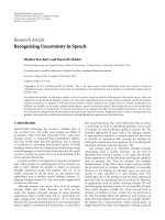
Fig. 3. Receiver operating characteristics for varying b - a.

Note that our test variable in (11) is
 
 
,
1

,min
1
11



N
t
i
N
t
y
N
dtw
N

which is a sample
average of N i.i.d. random variables that appear at the output of the nonlinearity y=h(w).
According to the central limit theorem (Papoulis & Pillai 2002) the probability distribution
function of such a sum approaches with increasing N, rapidly the Gaussian distribution
with mean
 
i
HyE
and variance
N
i
H
2


irrespective of the shape of the original distribution.
We can now evaluate the probability of correct detection (Van Trees 1971) as
 








,1
2
erf
2
1
2
exp
2
1
1
1
1
2
1
1
































H
Th
H

H
Th
yD
NHyETh
dy
NHyEy
N
dyHypP





(17)
Increasing b - a
Detection of echo generated in mobile phones 275

where Th is the threshold used in the test and erf denotes the error function
 


x
dttx
0
2
exp
2
)erf(

. Correspondingly the probability of fault detection is

 








.1
2
erf
2
1
2
exp
2
0
0
0
0
2
0
0
































H
Th
H
H
Th

yF
NHyETh
dy
NHyEy
N
dyHypP





(18)
The Receiver Operating Characteristic (ROC), which is the probability of correct detection
P
D
as a function of probability of fault alarm P
F
, is plotted in Fig. 3. The parameters used to
compute ROCs are N = 30, σ = 2 and β = 0.1. The distance between the endpoints of the
uniform density, b – a, varies from 4 to 12. One can see that the ROC curves approach the
upper left corner of the figure with increasing b – a.
It is also important to note that the detector derived in this chapter has a robust behavior.
The decision algorithm is piecewise linear in signal samples and in addition each entry of
the incoming signal is saturated at d, meaning that no single noise entry no matter how big it
is can influence the decision more than by d. Hence, the detector constitutes a robust test in
the terminology used in (Huber 2004).

5. Practical considerations

The detector, as given by equation (10) is not very convenient for implementation, as it

needs computation of a sum over all subframes with each new incoming subframe. To give
formula (10) a more convenient, recursive, form we define a set of distance metrics D, one
for each echo delay Δ of interest
     
 
.,min,
1



t
i
dlul
diTiTtctD


(19)
The distance metrics are functions of time t or more precisely the subframe number.
Computation of the distance metric can now easily be reformulated as a running sum i.e. at
any time t we compute the following distance metric for each of the delays of interest and
compare it with zero
       
 
.0,min,1,
0
1
H
H
dlul
dtTtTctDtD






(20)
Note that a large distance metric means that there is a similarity between the uplink and
downlink signals and the other way around, a small distance metric indicates that no
similarity has been found. Also note, that one can easily introduce a forgetting factor into
the recursive detector structure in order to gradually forget old data as it is customary in e.g.
adaptive algorithms (Haykin 2002). We are, however, not going to do this here. The echo is
detected if any of the distance metrics exceeds a certain threshold level, which is zero in this
case. The echo delay corresponds to  with largest associated distance metric,
 
,tD
.



Fig. 3. Receiver operating characteristics for varying b - a.

Note that our test variable in (11) is
 
 
,
1
,min
1
11




N
t
i
N
t
y
N
dtw
N

which is a sample
average of N i.i.d. random variables that appear at the output of the nonlinearity y=h(w).
According to the central limit theorem (Papoulis & Pillai 2002) the probability distribution
function of such a sum approaches with increasing N, rapidly the Gaussian distribution
with mean
 
i
HyE
and variance
N
i
H
2

irrespective of the shape of the original distribution.
We can now evaluate the probability of correct detection (Van Trees 1971) as
 









,1
2
erf
2
1
2
exp
2
1
1
1
1
2
1
1
































H
Th
H
H
Th
yD
NHyETh

dy
NHyEy
N
dyHypP





(17)
Increasing b - a
Recent Advances in Signal Processing276



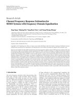
Fig.4. Histogram of pitch estimation errors. Echo path: single reflection and IRS filter, ERL =
-40dB. Near end noise at -60 dBm0


To answer this question a two minute long speech file that includes both male and female
voices at various levels was first coded with the AMR12.2 kbit/s mode codec and then
decoded. Then a simple echo path model consisting either of a single reflection or the IRS
filter (ITU-T G.191) was applied to the signal and the signal was coded again. Echo return
loss was varied between 30 and 40 dB. The estimated pitch was registered from both codecs
and compared. The pitch estimates were used only if the downlink power was above –40
dBm0 for the particular frame. A typical example is shown in Figure 4. The upper plot
shows the histogram of pitch estimation errors. A narrow peak can be observed around zero
and the histogram has long tails ranging from –125 to 125 (which are the limiting values for
differences between two pitch periods). The lower plot shows the Laplace probability
density function fitted to the middle part of the histograms. One can see that there is a

reasonable fit.


6.2 Detection performance
Recordings made with various mobile phones were used to examine the detection
performance. All the distance metrics in (20) were initialized to -50 and the echo was
declared to be present if at least one of the distance metrics became larger than zero. Validity

There are several practicalities that need to be added to the basic detector structure
derived in Section 3:
1. Speech signals are non-stationary and there is no point in running the detector if
the downlink speech is missing or has too low power to generate any echo. As a
practical limit, the distance metric is updated only if the down-link signal power is
above –30 dBm0.
2. By a similar reason there is a threshold on the down-link pitch gain. The threshold
is set to 10000.
3. The detection is only performed on “good” uplink frames i.e. SID frames and
corrupted frames are excluded.
4. It has been found in practice that c = 7 and d = 9 is a reasonable choice.
5. To allow fast detection of a spurious echo burst, the distance metrics are saturated
at –200 i.e. we always have


.200, tD

Additionally one can notice that the most common error in pitch estimation occurs at double
of the actual pitch period. This can be exploited to enhance the detector. In the particular
implementation this has been taken into account by adding a parallel channel to the detector
where the downlink pitch period is compared to half of the uplink pitch period
   

 
 
,0,
2
min,1,
0
1
11
H
H
dl
ul
dtT
tT
ctDtD













(21)
where the constants c

1
and d
1
are selected to be smaller than the corresponding constants c
and d in (20) to give a lower weight to the error channel as compared to the main channel.
Only one of the updates given by (20) and (21) is used each time t. The selected update is the
one that results in a larger increase of the distance metric.

6. Simulation results

Our simulation study is carried out with the aim of investigating how well the derived
detector works with speech signals. We first investigate if the distribution adopted in this
work can be justified. This is followed by some experiments clarifying detection
performance of the proposed algorithm using recordings made in an actual mobile network
and finally we investigate the resistance of the detector to disturbances.

6.1 Distribution of pitch estimation errors
In this section we investigate the distribution function of the pitch estimation errors. The
main question to answer is if the distribution function adopted in Section 3 is in accordance
with what can be observed in the simulations.
Detection of echo generated in mobile phones 277



Fig.4. Histogram of pitch estimation errors. Echo path: single reflection and IRS filter, ERL =
-40dB. Near end noise at -60 dBm0


To answer this question a two minute long speech file that includes both male and female
voices at various levels was first coded with the AMR12.2 kbit/s mode codec and then

decoded. Then a simple echo path model consisting either of a single reflection or the IRS
filter (ITU-T G.191) was applied to the signal and the signal was coded again. Echo return
loss was varied between 30 and 40 dB. The estimated pitch was registered from both codecs
and compared. The pitch estimates were used only if the downlink power was above –40
dBm0 for the particular frame. A typical example is shown in Figure 4. The upper plot
shows the histogram of pitch estimation errors. A narrow peak can be observed around zero
and the histogram has long tails ranging from –125 to 125 (which are the limiting values for
differences between two pitch periods). The lower plot shows the Laplace probability
density function fitted to the middle part of the histograms. One can see that there is a
reasonable fit.


6.2 Detection performance
Recordings made with various mobile phones were used to examine the detection
performance. All the distance metrics in (20) were initialized to -50 and the echo was
declared to be present if at least one of the distance metrics became larger than zero. Validity

There are several practicalities that need to be added to the basic detector structure
derived in Section 3:
1. Speech signals are non-stationary and there is no point in running the detector if
the downlink speech is missing or has too low power to generate any echo. As a
practical limit, the distance metric is updated only if the down-link signal power is
above –30 dBm0.
2. By a similar reason there is a threshold on the down-link pitch gain. The threshold
is set to 10000.
3. The detection is only performed on “good” uplink frames i.e. SID frames and
corrupted frames are excluded.
4. It has been found in practice that c = 7 and d = 9 is a reasonable choice.
5. To allow fast detection of a spurious echo burst, the distance metrics are saturated
at –200 i.e. we always have



.200,



tD

Additionally one can notice that the most common error in pitch estimation occurs at double
of the actual pitch period. This can be exploited to enhance the detector. In the particular
implementation this has been taken into account by adding a parallel channel to the detector
where the downlink pitch period is compared to half of the uplink pitch period
   
 
 
,0,
2
min,1,
0
1
11
H
H
dl
ul
dtT
tT
ctDtD














(21)
where the constants c
1
and d
1
are selected to be smaller than the corresponding constants c
and d in (20) to give a lower weight to the error channel as compared to the main channel.
Only one of the updates given by (20) and (21) is used each time t. The selected update is the
one that results in a larger increase of the distance metric.

6. Simulation results

Our simulation study is carried out with the aim of investigating how well the derived
detector works with speech signals. We first investigate if the distribution adopted in this
work can be justified. This is followed by some experiments clarifying detection
performance of the proposed algorithm using recordings made in an actual mobile network
and finally we investigate the resistance of the detector to disturbances.

6.1 Distribution of pitch estimation errors

In this section we investigate the distribution function of the pitch estimation errors. The
main question to answer is if the distribution function adopted in Section 3 is in accordance
with what can be observed in the simulations.
Recent Advances in Signal Processing278
6.3 Resistance to disturbances


Fig. 6. Evaluation of the detector in severe double talk conditions, mobile side male, network
side female.

Finally we check that the detector is not unnecessarily sensitive to disturbances. In echo
context the most common disturbance is so called double talk i.e. the situation when both
parties of the telephone conversation are talking at the same time. In this situation speech
from the near end side forms a strong disturbance to any algorithm that needs to cope with
echoes. The proposed detector algorithm was verified in a large number of simulations
involving speech signals from both sides of the connection and its double talk performance
was found to be good. This is expected as robustness against disturbances is built in the
algorithm in form of limited distance measure update in equation (20).
As another and perhaps somewhat spectacular demonstration of double talk performance,
we used two speech files with male and female voices speaking exactly the same sentences
the same time. The result is shown in Figure 6 with female voice from network side and
male voice from mobile side. In this case there are some fault echo detections initially, partly
caused by initialization of the distance metrics to –50. Duration of the fault detection is,
however, limited to the first two sentences (14 seconds) of the double talk. There was no
echo detected in the opposite scenario i.e. male voice from the mobile side and female voice
from the network side. Taking into account that it is very unlikely that in an actual

of the detection was verified by listening to the recorded file and comparing the listening
and detection results. The two were found to be in a good agreement with each other.

Fig. 5. Distance metrics (upper plot) and estimated delay (lower plot)

The delay was estimated as the one corresponding to the largest distance metric. As the
experiments were done with signals recorded in real mobile systems, the author lacks
knowledge of the true echo delays in the test cases. However, the estimates were proven in
practice to provide good enough estimates for usage in a practical echo removal device.
Let us finally note that the resolution of the delay estimate is 5 ms due to the 5 ms subframe
structure of the AMR speech codec.
A typical case with a mobile that produces echo is shown Figure 5. One can see that in this
example echo is detected and the delay estimate stabilizes after a couple of seconds to 165
ms, which is a reasonable echo delay for a GSM system.
Detection of echo generated in mobile phones 279
6.3 Resistance to disturbances


Fig. 6. Evaluation of the detector in severe double talk conditions, mobile side male, network
side female.

Finally we check that the detector is not unnecessarily sensitive to disturbances. In echo
context the most common disturbance is so called double talk i.e. the situation when both
parties of the telephone conversation are talking at the same time. In this situation speech
from the near end side forms a strong disturbance to any algorithm that needs to cope with
echoes. The proposed detector algorithm was verified in a large number of simulations
involving speech signals from both sides of the connection and its double talk performance
was found to be good. This is expected as robustness against disturbances is built in the
algorithm in form of limited distance measure update in equation (20).
As another and perhaps somewhat spectacular demonstration of double talk performance,
we used two speech files with male and female voices speaking exactly the same sentences
the same time. The result is shown in Figure 6 with female voice from network side and

male voice from mobile side. In this case there are some fault echo detections initially, partly
caused by initialization of the distance metrics to –50. Duration of the fault detection is,
however, limited to the first two sentences (14 seconds) of the double talk. There was no
echo detected in the opposite scenario i.e. male voice from the mobile side and female voice
from the network side. Taking into account that it is very unlikely that in an actual

of the detection was verified by listening to the recorded file and comparing the listening
and detection results. The two were found to be in a good agreement with each other.


Fig. 5. Distance metrics (upper plot) and estimated delay (lower plot)

The delay was estimated as the one corresponding to the largest distance metric. As the
experiments were done with signals recorded in real mobile systems, the author lacks
knowledge of the true echo delays in the test cases. However, the estimates were proven in
practice to provide good enough estimates for usage in a practical echo removal device.
Let us finally note that the resolution of the delay estimate is 5 ms due to the 5 ms subframe
structure of the AMR speech codec.
A typical case with a mobile that produces echo is shown Figure 5. One can see that in this
example echo is detected and the delay estimate stabilizes after a couple of seconds to 165
ms, which is a reasonable echo delay for a GSM system.
Recent Advances in Signal Processing280

telephone call both sides would talk the same sentences simultaneously we conclude that
the detector is reasonably resistant to double talk.

7. Conclusion

This chapter deals with the problem of processing AMR coded speech signals without
decoding them first. Importance of such algorithms arises from the fact that not all calls

need enhancement and even if they need the quality loss from decoding and coding speech
again may be higher than the potential improvement due to speech enhancement.
Processing the signals directly in the coded domain avoids this problem.
The chapter proposes a detector that can be used to detect presence of echo generated by
mobile phones and estimate its delay. The detector uses saturated absolute distance between
uplink and downlink pitch periods as a similarity measure and is hence a robust algorithm.
Performance of the detector was analysed and the equations for detection and error
probabilities were derived. Finally a good performance of the detector with real life signals
was demonstrated in our simulation study.

8. References

3GPP TS 26.090 V6.0.0 (2004-12) 3rd Generation Partnership Project; Technical Specification
Group Services and System Aspects; Mandatory Speech Codec speech processing
functions; Adaptive Multi-Rate (AMR) speech codec; Transcoding functions (Release 6).
Haykin, S. (2002) Adaptive Filter Theory, fourth edition, Prentice Hall
Huber, P. (2004) Robust Statistics, Wiley & Sons
ITU-T Recommendation G.160 (2008) Voice Enhancement devices
ITU-T Recommendation G.191, (2005) Software Tools for Speech and Audio Coding
Standardization
Kay, S. (1998) Fundamentals of Statistical Signal Processing, Volume II, Detection Theory, Prentice
Hall
Papoulis, A. and Pillai, S. U. (2002) Probability, Random Variables and Stochastic Processes,
Fourth edition, McGraw Hill
Perry, A. (2007) Fundamentals of Voice-Quality Engineering in Wireless Networks, Cambridge
University Press
Signal Processing, Volume 86, Issue 6, June 2006, Special issue on Applied Speech and Audio
Processing.
Sondhi, M and Berkley, D. (1980) Silencing Echoes in Telephone Network, Proc. IEEE, Vol.
68, No. 8, Aug. 1980 pp. 948-963.

Van Trees, H. L. (1971) Detection, Estimation, and Modulation Theory, Wiley & Sons
Application of the Vector Quantization Methods and
the Fused MFCC-IMFCC Features in the GMM based Speaker Recognition 281
Application of the Vector Quantization Methods and the Fused MFCC-
IMFCC Features in the GMM based Speaker Recognition
Sheeraz Memon, Margaret Lech, Namunu Maddage and Ling He
X

Application of the Vector Quantization Methods
and the Fused MFCC-IMFCC Features in the
GMM based Speaker Recognition

Sheeraz Memon, Margaret Lech, Namunu Maddage and Ling He
School of Electrical and Computer Engineering, RMIT University, Melbourne, Australia

1. Introduction

Speaker recognition system which identifies or verifies a speaker based on a person’s voice
is employed as biometric of high confidence. Over three decades of research, voice prints
have established very important security applications for the authentication and recognition
from voice channels. Recent years, speaker recognition community is putting more efforts to
further improve main factors such as robustness and the accuracy in the context
independent speaker recognition systems. Signal segmentation where the temporal
properties such as energy and pitch with in the speech signal frame is ideally considered
stationary, is a major step in speaker recognition systems. Another important area where
robustness can be acheived is identifying speaker characteristic sensitive feature extraction
methods. However the segmentation and feature extraction stages are examined by
modelling methods, thus speaker characteristic modelling is also an important state which
should be carefully designed. Effective improvements in above key steps subsequently
improve the robustness and accuracy of the speaker recognition system.

In this book chapter we evaluate the performances of the speaker recognition systems when
different feature settings and modelling techniques are applied for above mentioned step 2
and step 3 respectively. In general content sensitive features play a vital role in achieving the
globally optimized classification decisions. State of the art speaker recognition systems
extract acoustic features which capture the characteristics of the speech production system
such as pitch or energy contours, glottal waveforms, or formant amplitude and frequency
modulation and model them with statistical learning techniques. However Mel frequency
cepstral coefficients (MFCCs) have commonly being used to characterize the speaker
characteristics. In this chapter we compare effectiveness of Inverted MFCC and fused
MFCC-IMFCC features against solo MFCC feature for speaker recognition systems. It is
commonly assumed that the speaker characteristic distribution is Gaussian. Thus Gaussian
Mixture model is effectively used for speaker characteristics modelling in the literature. In
this chapter we examine different learning techniques for the representation of the
parameters in the GMM based speaker models. Vector Quantization (VQ) techniques
effectively cluster the information distributions and reduce the effects of noise. Its found VQ
techniques improve the robustness of speaker recognition systems which are deployed at
17
Recent Advances in Signal Processing282

methods improve the GMM performance. The relation between number of vector
quantization methods and EM is established in (Ethem A.,1998). To overcome the problem
of local maxima caused by EM algorithm with an annealing approach is suggested in (Ueda,
N. & R. Nakano, 1998).


Fig. 1. overview of speaker verification systems

Vector Quantization (VQ) based speaker verification has been recognized as a successful
method in the field of speaker recognition systems. A number of attempts have been made
to use VQ methods with the GMM to optimize the performance of a speaker recognition

system (Jialong et. Al, 1997) and (Singh et. al, 2003). The basic idea of VQ is to compress a
large number of short term spectral vectors into a smaller set of code vectors. Until the
development of GMM, vector quantization techniques were the most often applied methods
in the field of speaker verification.
In this chapter we apply ITVQ algorithm (Tue et al.,2005), beside K-means and LBG VQ
processes to estimate EM parameters. The ITVQ algorithm, which incorporates the
Information Theoretic principles into the VQ process, was found to be the most efficient VQ
algorithm (Sheeraz M. & Margaret L, 2008).

4. Feature Extraction Methods

Feature extraction is useful in speech (Davis, S. B. & P. Mermelstein,1980) and speaker
recognition and the study of feature extraction has remained a core of research. A number of
studies best support Mel-frequency cepstrum coefficients (MFCCs) (Reynolds, D. A. , 1994)
and it does produce good results in most of the situations. In other studies, feature
extraction based on pitch or energy contours (Peskin B. et al.,2003), glottal waveforms

different noisy environments. We propose several VQ methods to optimize GMM
parameters (mean, covariance, and mixture weight). However expectation maximization
(EM) algorithm is commonly used in the literature for the GMM parameter optimization.
Thus we compare the performances of VQ based GMM –speaker modelling algorithms, K-
means, LBG (Linde Buzo and Gray) and Information theoretic vector quantization (ITVQ)
with EM-GMM setup in the speaker recognition.
The study includes speaker verification tests performed on the NIST2004 Speaker
Recognition evaluation Corpus. NIST2004 SRE consists of conversational telephone speech.
Thus performance evaluation of proposed methods using this corpus allows us to analyse
and validate the results with high confidence. The results are presented using detection
error trade-off (DET) plots showing the miss probability against the false alarm probability;
a number of tables are also presented to compare the recognition rates based on different
combination of these techniques.

2. Speaker Recognition

Speaker Recognition is a biometric based identity process where a person’s identity is
verified by the voice of a person. Biometrics based verification has received much attention
in the recent times as such characteristics come natural to each individual and they are not
required to be memorised, like passwords and personal identification numbers.
The speaker recogniton can be further classified in speaker identification and verification.
Identification deals when a person is needed to verify from a group of people, however in
verification task a person is accepted or rejected based on a claimant’s identity.
In text-independent speaker verification the speaker is not bound to say a specific phrase to
be identified but he/she is free to utter any sentence. However when we are dealing with
text-dependent speaker recogntion the person is bound to utter a pre-defined phrase.
The speaker verification system comprises of three stages (see Fig. 1), in the first stage pre-
processing and feature extraction is performed over a database of speakers. The second step
addresses establishment of speaker models; where vectors representing speakers
distinguishing characteristics are generated this corresponds to finding the distributions of
feature vectors. The third step is of decision, which confirms or rejects the claimed identity
of a speaker. In this stage the test set is also performed which includes the pre-processing
and feature extraction of the test speaker and inputs to the classifier.
The introduction of the adapted Gaussian mixture models (Reynolds et al.,2000) with the
introduction of UBM-GMM with MAP adaptation has established very good results on
NIST evaluations. The use of expectation maximization (EM) optimization procedure is
widely adapted to obtain the iterative updates for gaussian distributions. However EM
encounters a number of problems, such as local convergence, mean adaptations etc. A
number of EM variants are also proposed recently (Ueda, N. & R. Nakano, 1998), (Hedelin,
P. Skoglund, J., 2000), (Ververidis, D. Kotropoulos, C.,2008) and (Ethem A.,1998).


3. Vector Quantization and EM based GMM

The study in (Hedelin, P. Skoglund, J., 2000) proposes how vector quantization based on
GMM enhances the performance. A number of statistical tests are conducted in (Ververidis,
D. Kotropoulos, C.,2008), it suggests around seven EM variants which under enhanced
Application of the Vector Quantization Methods and
the Fused MFCC-IMFCC Features in the GMM based Speaker Recognition 283

methods improve the GMM performance. The relation between number of vector
quantization methods and EM is established in (Ethem A.,1998). To overcome the problem
of local maxima caused by EM algorithm with an annealing approach is suggested in (Ueda,
N. & R. Nakano, 1998).


Fig. 1. overview of speaker verification systems

Vector Quantization (VQ) based speaker verification has been recognized as a successful
method in the field of speaker recognition systems. A number of attempts have been made
to use VQ methods with the GMM to optimize the performance of a speaker recognition
system (Jialong et. Al, 1997) and (Singh et. al, 2003). The basic idea of VQ is to compress a
large number of short term spectral vectors into a smaller set of code vectors. Until the
development of GMM, vector quantization techniques were the most often applied methods
in the field of speaker verification.
In this chapter we apply ITVQ algorithm (Tue et al.,2005), beside K-means and LBG VQ
processes to estimate EM parameters. The ITVQ algorithm, which incorporates the
Information Theoretic principles into the VQ process, was found to be the most efficient VQ
algorithm (Sheeraz M. & Margaret L, 2008).

4. Feature Extraction Methods

Feature extraction is useful in speech (Davis, S. B. & P. Mermelstein,1980) and speaker

recognition and the study of feature extraction has remained a core of research. A number of
studies best support Mel-frequency cepstrum coefficients (MFCCs) (Reynolds, D. A. , 1994)
and it does produce good results in most of the situations. In other studies, feature
extraction based on pitch or energy contours (Peskin B. et al.,2003), glottal waveforms
Recent Advances in Signal Processing284

If N
F
denotes the number of filters in the filter bank, then
1
0
}{


F
i
N
ib
k
are the boundary points
of the filters. The boundary points for each filter i (i=1,.2, , N
F
) are calculated as equally
spaced points in the Mel scale using the following formula,





















1
)()(
)(
F
lowmelhighmel
lowmelmel
s
b
N
ffffi
fff
f
M
k
i

(4)
Where, f
s
is the sampling frequency in Hz and f
low
=f
s
/M and f
high
= S
F
/2 are the low and high
frequency boundaries of the filter bank, respectively.
Step.3: In the next step, the output energies E(i) (i=1,.2, , N
F
) of the Mel-scaled band-pass
filters are calculated as a sum of the signal energies
2
)(kX
falling into a given Mel frequency
band weighted by the corresponding frequency response
)(k
i

. This is given as,



2
1

2
)()()(
S
M
x
i
kkXiE


(5)
Where M
s
is the number of DFT bins falling into the i
th
filter.
Step.4: Finally, the Discrete Cosine Transform (DCT) of the log of the filter bank output
energies E(i) (i=1,.2, , N
F
) is calculated yielding the final set of the MFCC coefficients C
m
,
given as


















F
N
l
F
m
N
l
miE
N
C
F

.
2
12
.cos.)]1(log[
2
1
0

(6)
Where, m=0,1,2, ,R-1, and R is the desired number of the Mel Frequency Cepstral
Coefficients.

4.2 Inverted Mel-frequency cepstral coefficients (MFCC)
The MFCC represent the information perceived by the human auditory system while the
Inverse Mel Frequency Cepstral Coefficients capture the information which could have been
missed by the MFCC (Yegnanarayana, B. et. al, 2005). The Inverted Mel Scale, which is
shown as a dashed line in Fig.4, is defined by a filter bank structure that follows the
opposite path to that of MFCC. The inverted filter bank structure can be generated by
flipping the original filter bank around the mid frequency point f
c
, of the filter bank
frequency range (i.e. f
c
=(f
high
- f
low
)/2).



(Plumpe, M. D. Et. al, 1999), or formant amplitude and frequency modulation (Jankowski C.
R. jr. et al.,1996) are proposed, and good performance has been shown.
In their recent research (Sandipan, C. & Ghoutam, S.,2008) suggested, that the classification
results can be significantly improved when the MFCC method is fused with the Inverse
MFCC (IMFCC). This is because the IMFCC helps to capture the speaker specific
information lying in the higher frequency range of the spectrum, which is largely ignored by
the MFCC feature extraction method.

4.1 Mel-frequency cepstral coefficients (MFCC)
The primary concern of describing the MFCC algorithm here is to clearly map the working
of Inverted MFCC and later in this chapter their fusion as a feature extraction set for GMM
based on EM, K-means, LBG and ITVQ classifier. MFCC algorithm has been widely used for
both the speech and speaker recognition in the recent years as it is designed keeping the
human perception of listening as the core concern. According to psychophysical studies
(Shaughnessy, D. O.,1987), human perception of the frequency content of sounds follows a
subjectively defined nonlinear scale called the Mel scale (Gold, B. & Morgan, N.,2002) (Fig.
2). Mel scale is defined as a logarithmic scale of frequency based on human pitch perception.
Equal intervals in Mel units correspond to equal pitch intervals. It is given by,







700
1log2595
10
f
f
mel

(1)
Where f
mel
is the subjective pitch in Mels corresponding to f which is the actual frequency in
Hz. This leads to the definition of MFCC, a baseline acoustic feature for Speech and Speaker

Recognition applications, can be calculated by following steps.
Step.1: Let
M
n
nx
1
)}({

represent a time-domain frame of pre-processed speech. The speech
samples x(n) are first transformed to the frequency domain by the M-point Discrete Fourier
Transform (DFT) and then the signal energy is calculated as,
2
1
2
2
).(|)(|












M
n

M
nxj
enxkX



(2)
Where, k=1,2, ,M and X(k) = DFT(x(n)).
Step.2: This is followed by the construction of a filter bank with triangular frequency
responses centered at equally spaced points on the Mel scale. Fig. 2 shows the frequency
response of the i
th
filter. The frequency response
)(k
i

of this filter is calculated using
Eq.(3).


k
i



























1
1
1
1
1
1
1
1
0
0
i
ii

ii
i
ii
ii
i
i
b
bb
bb
b
bb
bb
b
b
kkfor
kkkfor
kk
kk
kkkfor
kk
kk
kkfor




(3)
Application of the Vector Quantization Methods and
the Fused MFCC-IMFCC Features in the GMM based Speaker Recognition 285

If N
F
denotes the number of filters in the filter bank, then
1
0
}{


F
i
N
ib
k
are the boundary points
of the filters. The boundary points for each filter i (i=1,.2, , N
F
) are calculated as equally
spaced points in the Mel scale using the following formula,





















1
)()(
)(
F
lowmelhighmel
lowmelmel
s
b
N
ffffi
fff
f
M
k
i

(4)
Where, f
s
is the sampling frequency in Hz and f
low
=f

s
/M and f
high
= S
F
/2 are the low and high
frequency boundaries of the filter bank, respectively.
Step.3: In the next step, the output energies E(i) (i=1,.2, , N
F
) of the Mel-scaled band-pass
filters are calculated as a sum of the signal energies
2
)(kX
falling into a given Mel frequency
band weighted by the corresponding frequency response
)(k
i

. This is given as,



2
1
2
)()()(
S
M
x
i

kkXiE


(5)
Where M
s
is the number of DFT bins falling into the i
th
filter.
Step.4: Finally, the Discrete Cosine Transform (DCT) of the log of the filter bank output
energies E(i) (i=1,.2, , N
F
) is calculated yielding the final set of the MFCC coefficients C
m
,
given as


















F
N
l
F
m
N
l
miE
N
C
F

.
2
12
.cos.)]1(log[
2
1
0


(6)
Where, m=0,1,2, ,R-1, and R is the desired number of the Mel Frequency Cepstral
Coefficients.

4.2 Inverted Mel-frequency cepstral coefficients (MFCC)
The MFCC represent the information perceived by the human auditory system while the

Inverse Mel Frequency Cepstral Coefficients capture the information which could have been
missed by the MFCC (Yegnanarayana, B. et. al, 2005). The Inverted Mel Scale, which is
shown as a dashed line in Fig.4, is defined by a filter bank structure that follows the
opposite path to that of MFCC. The inverted filter bank structure can be generated by
flipping the original filter bank around the mid frequency point f
c
, of the filter bank
frequency range (i.e. f
c
=(f
high
- f
low
)/2).



(Plumpe, M. D. Et. al, 1999), or formant amplitude and frequency modulation (Jankowski C.
R. jr. et al.,1996) are proposed, and good performance has been shown.
In their recent research (Sandipan, C. & Ghoutam, S.,2008) suggested, that the classification
results can be significantly improved when the MFCC method is fused with the Inverse
MFCC (IMFCC). This is because the IMFCC helps to capture the speaker specific
information lying in the higher frequency range of the spectrum, which is largely ignored by
the MFCC feature extraction method.

4.1 Mel-frequency cepstral coefficients (MFCC)
The primary concern of describing the MFCC algorithm here is to clearly map the working
of Inverted MFCC and later in this chapter their fusion as a feature extraction set for GMM
based on EM, K-means, LBG and ITVQ classifier. MFCC algorithm has been widely used for
both the speech and speaker recognition in the recent years as it is designed keeping the

human perception of listening as the core concern. According to psychophysical studies
(Shaughnessy, D. O.,1987), human perception of the frequency content of sounds follows a
subjectively defined nonlinear scale called the Mel scale (Gold, B. & Morgan, N.,2002) (Fig.
2). Mel scale is defined as a logarithmic scale of frequency based on human pitch perception.
Equal intervals in Mel units correspond to equal pitch intervals. It is given by,







700
1log2595
10
f
f
mel

(1)
Where f
mel
is the subjective pitch in Mels corresponding to f which is the actual frequency in
Hz. This leads to the definition of MFCC, a baseline acoustic feature for Speech and Speaker
Recognition applications, can be calculated by following steps.
Step.1: Let
M
n
nx
1

)}({

represent a time-domain frame of pre-processed speech. The speech
samples x(n) are first transformed to the frequency domain by the M-point Discrete Fourier
Transform (DFT) and then the signal energy is calculated as,
2
1
2
2
).(|)(|












M
n
M
nxj
enxkX


(2)
Where, k=1,2, ,M and X(k) = DFT(x(n)).
Step.2: This is followed by the construction of a filter bank with triangular frequency
responses centered at equally spaced points on the Mel scale. Fig. 2 shows the frequency
response of the i
th
filter. The frequency response
)(k
i

of this filter is calculated using
Eq.(3).


k
i



























1
1
1
1
1
1
1
1
0
0
i
ii
ii
i
ii
ii
i
i

b
bb
bb
b
bb
bb
b
b
kkfor
kkkfor
kk
kk
kkkfor
kk
kk
kkfor




(3)
Recent Advances in Signal Processing286


Fig. 4. Subjective pitch in Mels vs. frequency in Hz.



2
1

2
)(
ˆ
)()(
ˆ
S
M
x
i
kkYiE


(9)
Finally, the DCT of the log filter bank energies is calculated, and the final Inverted Mel
Frequency Cepstral Coefficients
m
C
ˆ
are given as,


















F
N
l
F
m
N
l
miE
N
C
F

2
12
cos.)]1(
ˆ
log[
2
ˆ
1
0

(10)
Where, m=0,1,2, ,R-1, and R is the number of the Inverted Mel Frequency Cepstral

Coefficients.

4.3 Fusion of MFCC and IMFCC
The idea of combining the classifiers to optimize the decision making process has been
successfully applied in the fields of pattern recognition and classification (Mashao, DJ. &
Skosan, M, 2006), (Murty, KSR. & Yegnanarayana, B.,2006). If the information supplied to
the classifiers is complementary, such as the case of MFCC and IMFCC, the classification
process could be largely improved (Sandipan, C. & Ghoutam, S.,2008) , (Chakroborty, S et.
al, 2006).
The MFCC and the IMFCC feature vectors, containing complimentary information about the
speakers, were supplied to a given classifier independently and the classification results for
the MFCC features and for the IMFCC were fused in order to obtain optimal decisions in the
process of speaker verification. A uniform weighted sum rule was adopted to fuse the scores
from the two classifiers. If D
MFCC
denotes the classification score based on the MFCC, and
D
IMFCC
denotes the classification score based on the IMFCC, then the combined score for the
m
th
speaker was given as,
IMFCCMFCCm
DDD )1(






(11)
The constant value of ω = 0.5 was used in all cases. The speaker class was determined as,


m
m
class
Dm maxarg

(12)


Fig. 2. Implementation structure of MFCC











1i
b
k
b
k
1i

b
k
Fig.3. Response of a Mel scale Filter

The frequency responses


k
i

ˆ
(i=1,2, , N
F
) for the inverted filter bank are given as,
 








k
M
k
iN
i
F
1

2
ˆ
1

(7)
For a given frequency f in Hz, the corresponding inverted Mel-scale frequency
)(
ˆ
ff
mel
can be
calculated as,








700
25.4031
1log25952860.2195)(
ˆ
10
f
ff
mel

(8)

The energies of the inverted filters outputs can be determined in the same way as for the
non-inverted filters, i.e.,
DFT of short time
analyzed signal
Construction of
Filter Bank
Log Amplitude
above Mel scale
DCT of Mel-Log
Amplitudes
C
m
Speech
sample i/p
DFT Coefficient index
Application of the Vector Quantization Methods and
the Fused MFCC-IMFCC Features in the GMM based Speaker Recognition 287


Fig. 4. Subjective pitch in Mels vs. frequency in Hz.



2
1
2
)(
ˆ
)()(
ˆ

S
M
x
i
kkYiE


(9)
Finally, the DCT of the log filter bank energies is calculated, and the final Inverted Mel
Frequency Cepstral Coefficients
m
C
ˆ
are given as,


















F
N
l
F
m
N
l
miE
N
C
F

2
12
cos.)]1(
ˆ
log[
2
ˆ
1
0

(10)
Where, m=0,1,2, ,R-1, and R is the number of the Inverted Mel Frequency Cepstral
Coefficients.

4.3 Fusion of MFCC and IMFCC
The idea of combining the classifiers to optimize the decision making process has been
successfully applied in the fields of pattern recognition and classification (Mashao, DJ. &

Skosan, M, 2006), (Murty, KSR. & Yegnanarayana, B.,2006). If the information supplied to
the classifiers is complementary, such as the case of MFCC and IMFCC, the classification
process could be largely improved (Sandipan, C. & Ghoutam, S.,2008) , (Chakroborty, S et.
al, 2006).
The MFCC and the IMFCC feature vectors, containing complimentary information about the
speakers, were supplied to a given classifier independently and the classification results for
the MFCC features and for the IMFCC were fused in order to obtain optimal decisions in the
process of speaker verification. A uniform weighted sum rule was adopted to fuse the scores
from the two classifiers. If D
MFCC
denotes the classification score based on the MFCC, and
D
IMFCC
denotes the classification score based on the IMFCC, then the combined score for the
m
th
speaker was given as,
IMFCCMFCCm
DDD )1(




(11)
The constant value of ω = 0.5 was used in all cases. The speaker class was determined as,


m
m
class

Dm maxarg

(12)


Fig. 2. Implementation structure of MFCC











1i
b
k
b
k
1i
b
k
Fig.3. Response of a Mel scale Filter

The frequency responses



k
i

ˆ
(i=1,2, , N
F
) for the inverted filter bank are given as,
 








k
M
k
iN
i
F
1
2
ˆ
1

(7)
For a given frequency f in Hz, the corresponding inverted Mel-scale frequency
)(

ˆ
ff
mel
can be
calculated as,








700
25.4031
1log25952860.2195)(
ˆ
10
f
ff
mel

(8)
The energies of the inverted filters outputs can be determined in the same way as for the
non-inverted filters, i.e.,
DFT of short time
analyzed signal
Construction of
Filter Bank
Log Amplitude

above Mel scale
DCT of Mel-Log
Amplitudes
C
m
Speech
sample i/p
DFT Coefficient index
Recent Advances in Signal Processing288


b. Partition calculation. Given the codebook Y
m
, the partition P(Y
m
) is calculated according
to the nearest neighbour condition, given by
},, ,2,1
),,(),(:{
ijNj
yxdyxdXxS
C
jii




i=1,2,….,N
C
.

(14)
c. Termination condition check. The quantizer distortion (D
m
= D({Y
m
,P(Ym)}) is calculated
according to following equation.
 
 

P
C
N
p
N
i
i
P
pp
P
D
N
xqxd
N
SYDMQE
1 1
1
))(,(
1

}),({


(15)
Where D
i
indicates the total distortion of i
th
cell.
If


 mmm
DDD /)(
1
then the optimization ends and Y
m
is the final returned codebook.
d. New codebook calculation. Given the partition P(Y
m
), the new codebook is calculated
according to the Centroid condition. In symbols:
Y
m+1
= X (P(Y
m
)) (16)
After, the counter m is increased by one and the procedure follows from step b.

5.3 Information Theoretic VQ

The Vector Quantization methods are commonly used in the process of feature
classification. The ITVQ (Tue, L. et. al, 2005) algorithm uses a new set of concepts from
information theory and provides a computationally very efficient technique, which
eliminates many disadvantages of classical vector quantization algorithms. Unlike LBG, this
algorithm relies on minimization of a well defined cost function. The cost function used in
LBG and K-means algorithms is defined as an average distortion (or distance), and as such,
it is very complex and may contain discontinuities making the application of traditional
optimization procedures very difficult (Erwin, E. et. al, 1991).
According to the information theory a distance minimization is equivalent to the
minimization of the divergence between distribution of data and distribution of code
vectors. Both distributions can be estimated using the Parzen density estimator method
(Tue, L. et. al, 2005).
The ITVQ algorithm is based on the principle of minimizing the divergence between Parzen
estimator of the code vectors density distributions and a Parzen estimator of the data
distribution. The Parzen density estimator is given as,
   



N
i
i
xxK
N
xp
1
1


(17)

Where K(.) is the Gaussian Kernel, x is the independent variable for which we seek the
estimate and x
i
represents the data points. The Parzen estimate of the data has N kernels,
where N is the number of data points, and the Parzen estimator of the code vectors has M
kernels, where M is the number of code vectors and M<<N.
The density estimation is followed by minimization of the divergence between data points
and centroids. In order to minimize the divergence between the data points distribution a(x)
and the centroids distribution b(x), the following expression is minimized.


 



dxxbdxxbxadxxa
xbxaD
SC
)(log)()(log2)(log
)(),(
22

(18)

5. Vector Quantization (VQ) Methods

In this section of the chapter a number of VQ procedures are described, which have been
used to optimize the EM parameters for GMM modelling.

5.1 K-means Method

It is an algorithm to classify or to group data based on attributes/features into K number of
group. K is positive integer number. The grouping is done by minimizing the sum of
squares of distances between data and the corresponding cluster centroid. Thus, the purpose
of K-mean clustering is to classify the data. K-means algorithm (Furui, S., 1989) was
developed for vector quantization codebook generation. It represents each cluster by the
mean of the cluster. Assume a set of vectors X={x
1
,x
2
,x
3
,… ,x
T
} is to be divided into M
clusters represented by their mean vectors {µ
1
, µ
2
, µ
3
,…, µ
M
} the objective of K-means
algorithm is to minimize the total distortion given by,



T
t
it

M
i
xdistortiontotal
11
_


(13)
K-means is an iterative approach; in each successive iteration it redistributes the vectors in
order to minimize the distortion. The procedure is outlined below:
(a) Initialize the randomized centroids as the means of M clusters.
(b) Data points are associated with the nearest centroid.
(c) The centroids are moved to the centre of their respective clusters.
(d) Steps b & c are repeated until a suitable level of convergence has been reached, i.e.
the distortion is minimized.
When the distortion is minimized, redistribution does not result in any movement of vectors
among the clusters. This could be used as an indicator to terminate the algorithm. The total
distortion can also be used as an indicator of convergence of the algorithm. Upon
convergence, the total distortion does not change as a result of redistribution. It is to be
noted that in each iteration, K-means estimates the means of all the M clusters.

5.2 LBG Method
The LBG algorithm is a finite sequence of steps in which, at every step, a new quantizer,
with a total distortion less or equal to the previous one, is produced. We can distinguish two
phases, the initialization of the codebook and its optimization. The codebook optimization
starts from an initial codebook and, after some iterations, generates a final codebook with a
distortion corresponding to a local minimum. The following are the steps for LBG
algorithm.

a. Initialization. The following values are fixed:

• N
C
: number of codewords;
• ε ≥ 0: precision of the optimization process;
• Y
0
: initial codebook;
• X = {x
j
; j = 1 , ,N
P
}: input patterns;
Further, the following assignments are made:
• m = 0; where m is the iteration number.
• D
−1
= +∞; where D is the minimum quantization error calculated at every m
th
iteration.
Application of the Vector Quantization Methods and
the Fused MFCC-IMFCC Features in the GMM based Speaker Recognition 289


b. Partition calculation. Given the codebook Y
m
, the partition P(Y
m
) is calculated according
to the nearest neighbour condition, given by
},, ,2,1

),,(),(:{
ijNj
yxdyxdXxS
C
jii



i=1,2,….,N
C
.

(14)
c. Termination condition check. The quantizer distortion (D
m
= D({Y
m
,P(Ym)}) is calculated
according to following equation.
 
 

P
C
N
p
N
i
i
P

pp
P
D
N
xqxd
N
SYDMQE
1 1
1
))(,(
1
}),({


(15)
Where D
i
indicates the total distortion of i
th
cell.
If


 mmm
DDD /)(
1
then the optimization ends and Y
m
is the final returned codebook.
d. New codebook calculation. Given the partition P(Y

m
), the new codebook is calculated
according to the Centroid condition. In symbols:
Y
m+1
= X (P(Y
m
)) (16)
After, the counter m is increased by one and the procedure follows from step b.

5.3 Information Theoretic VQ
The Vector Quantization methods are commonly used in the process of feature
classification. The ITVQ (Tue, L. et. al, 2005) algorithm uses a new set of concepts from
information theory and provides a computationally very efficient technique, which
eliminates many disadvantages of classical vector quantization algorithms. Unlike LBG, this
algorithm relies on minimization of a well defined cost function. The cost function used in
LBG and K-means algorithms is defined as an average distortion (or distance), and as such,
it is very complex and may contain discontinuities making the application of traditional
optimization procedures very difficult (Erwin, E. et. al, 1991).
According to the information theory a distance minimization is equivalent to the
minimization of the divergence between distribution of data and distribution of code
vectors. Both distributions can be estimated using the Parzen density estimator method
(Tue, L. et. al, 2005).
The ITVQ algorithm is based on the principle of minimizing the divergence between Parzen
estimator of the code vectors density distributions and a Parzen estimator of the data
distribution. The Parzen density estimator is given as,
   




N
i
i
xxK
N
xp
1
1


(17)
Where K(.) is the Gaussian Kernel, x is the independent variable for which we seek the
estimate and x
i
represents the data points. The Parzen estimate of the data has N kernels,
where N is the number of data points, and the Parzen estimator of the code vectors has M
kernels, where M is the number of code vectors and M<<N.
The density estimation is followed by minimization of the divergence between data points
and centroids. In order to minimize the divergence between the data points distribution a(x)
and the centroids distribution b(x), the following expression is minimized.


 



dxxbdxxbxadxxa
xbxaD
SC
)(log)()(log2)(log

)(),(
22

(18)

5. Vector Quantization (VQ) Methods

In this section of the chapter a number of VQ procedures are described, which have been
used to optimize the EM parameters for GMM modelling.

5.1 K-means Method
It is an algorithm to classify or to group data based on attributes/features into K number of
group. K is positive integer number. The grouping is done by minimizing the sum of
squares of distances between data and the corresponding cluster centroid. Thus, the purpose
of K-mean clustering is to classify the data. K-means algorithm (Furui, S., 1989) was
developed for vector quantization codebook generation. It represents each cluster by the
mean of the cluster. Assume a set of vectors X={x
1
,x
2
,x
3
,… ,x
T
} is to be divided into M
clusters represented by their mean vectors {µ
1
, µ
2
, µ

3
,…, µ
M
} the objective of K-means
algorithm is to minimize the total distortion given by,



T
t
it
M
i
xdistortiontotal
11
_


(13)
K-means is an iterative approach; in each successive iteration it redistributes the vectors in
order to minimize the distortion. The procedure is outlined below:
(a) Initialize the randomized centroids as the means of M clusters.
(b) Data points are associated with the nearest centroid.
(c) The centroids are moved to the centre of their respective clusters.
(d) Steps b & c are repeated until a suitable level of convergence has been reached, i.e.
the distortion is minimized.
When the distortion is minimized, redistribution does not result in any movement of vectors
among the clusters. This could be used as an indicator to terminate the algorithm. The total
distortion can also be used as an indicator of convergence of the algorithm. Upon
convergence, the total distortion does not change as a result of redistribution. It is to be

noted that in each iteration, K-means estimates the means of all the M clusters.

5.2 LBG Method
The LBG algorithm is a finite sequence of steps in which, at every step, a new quantizer,
with a total distortion less or equal to the previous one, is produced. We can distinguish two
phases, the initialization of the codebook and its optimization. The codebook optimization
starts from an initial codebook and, after some iterations, generates a final codebook with a
distortion corresponding to a local minimum. The following are the steps for LBG
algorithm.

a. Initialization. The following values are fixed:
• N
C
: number of codewords;
• ε ≥ 0: precision of the optimization process;
• Y
0
: initial codebook;
• X = {x
j
; j = 1 , ,N
P
}: input patterns;
Further, the following assignments are made:
• m = 0; where m is the iteration number.
• D
−1
= +∞; where D is the minimum quantization error calculated at every m
th
iteration.

Recent Advances in Signal Processing290

6.2 GMM with VQ
Although EM algorithm performs well but the literature has suggested that it suffers with
some of the problems which can enhance its performance for pattern recognition
applications such as speaker recognition (Ueda, N. & R. Nakano, 1998). The areas where the
performance improvement can be achieved are listed below.
1. The number of mixtures is mostly set a priori.
2. The initialization procedure applied to set the parameters affects the final result.
3. EM converges to local optima instead of global optima.
Thus investigation of alternative training algorithms is unavoidable. However this may
include either modifying the standard EM steps or by proposing enhanced optimization
procedures. We in this paper propose the use of several VQ methods to replace the
maximization step of EM algorithm. At each EM iteration expectation is set which is given
by,


 









1
2/1
1

2/1
)())(2/1(exp
)())(2/1(exp
j
lk
T
lkj
l
l
j
jk
T
jkjj
kj
xxg
xxg
h




(22)
The above equation is the evaluation of a speaker model at each EM iteration. The
numerator is the pdf of a target model and the denominator is the sum of all the pdf’s.
However the next part of EM based GMM is to obtain the iterative updates where we
propose to use the cost function of VQ methods. We apply the clustering techniques such as
K-means, LBG and ITVQ to optimize the means. However the covariances are computed as
evaluated in the initialization procedure, however based on the new clusters/distribution of
the speaker data. The iterative weights are the updates from the new expectation h
kj

as
evaluated in the EM procedure (see equation 22).



k
n
kj
n
j
h
n
g
)()1(
1


(23)
The K-means algorithm has been applied for finding a robust model approximation to the
GMM in (Singh et. al, ,2003) and (Pelecanos et. al, 2000). Hence we are using a number of
vector quantization algorithms including K-means, LBG and recently designed ITVQ to
investigate its suitability to avoid local convergence when using EM algorithm. We also
compare the performance of ITVQ over other vector quantization approaches.
How the cost minimization procedure is implemented for each clustering technique is
described in section 2 and the distortion function for each the clustering techniques are
listed in equations (1), (3) and (11) respectively.
A multi-dimensional Gaussian is calculated using the mean and variance statistics from the
test vectors in each code vector region, with the training vectors already grouped into their
code books. An approximation of the GMM is determined by estimating the mixture
weights p

k
, means μ
k
, and covariances ∑
k
. Each mean μ
k
is assigned to its corresponding
code vector,
k
c

. The covariance matrix
k

for each GMM is calculated from the variances of
the vector observations in each code vector region. To achieve the optimal approximation
the feature vectors need to be well clustered and the VQ based GMM also need to have the
features uncorrelated, for many applications including SV it is difficult to satisfy this
condition, however by attempting to match these requirements, model estimation errors
could be minimised. Normalization techniques (Mariethoz, J. & S. Bengio, 2005), (Barras, C.
& J. Gauvain, 2003) are also applied for this purpose to reduce the mismatch of features.

Where, a(x) and b(x) denote the Parzen density estimates for the data and centroids,
respectively.
The cost function in Eq. (18) is minimized through a gradient descent search, which
iteratively changes the positions of centroids until the decrease rate of the cost value
becomes sufficiently small. The first term in Eq.(18),

dxxa )(log

2
,represents the Renyi’s
quadratic entropy of data points, the third term,

dxxb )(log
2
, represents the Renyi’s
quadratic entropy of centroids, and the second term,

 dxxbxa )()(log2
, is the 2log of the
cross information potential between the densities of the centroids and the data. Since the
entropy of the data points remains constant during the iterations, the minimization of the
cost function in Eq. (18) is equivalent to the maximization of the sum of the entropy of the
centroids and the cross information potential between the densities of the centroids and the
data.
As explained in more detail in (Tue, L. et. al, 2005), a typical ITVQ algorithm makes use of
an annealing procedure, which allows the algorithm to escape from local minima.

6. Gaussian Mixture Models

In this section of the chapter we describe the modelling methods. GMM use EM procedure
for the optimization however the use of VQ methods is proposed here.

6.1 GMM with EM
The Gaussian Mixture Model (GMM) (Douglas, A.R., 1995) with Expectation maximization
is a feature modeling and classification algorithm widely used in the speech-based pattern
recognition, since it can smoothly approximate a wide variety of density distributions.
The probability density function (pdf) drawn from the GMM is a weighted sum of M
component densities given as,

)()|(
1
xxp
b
p
k
k
M
k





(19)
Where x is a D-dimensional random vector, b
k
(x), k =1… M are the component
densities and p
k
, k =1… M are the mixture weights. Each component density is a D-variate
Gaussian function of the form
 
 
   











1
'
2/1
2/
2
1
exp
2
1
i
kk
k
D
k
xxx
b



(20)
Where µ
i
is the mean vector and ∑ is the covariance matrix. The mixture weights satisfy the
constraint that




M
k
k
p
1
1
.The complete Gaussian mixture density is the collection of the
mean vectors, covariance matrices and mixture weights from all components densities,
Mkp
kkk
, ,1},,,{ 





(21)
Each class is represented by a mixture model and is referred by the class model λ.
The Expectation Maximization (EM) algorithm is most commonly used to iteratively derive
class models. The EM algorithm initialized with a speaker model

and estimates at each
iteration a new model

such that






|| XpXp 
.

Application of the Vector Quantization Methods and
the Fused MFCC-IMFCC Features in the GMM based Speaker Recognition 291

6.2 GMM with VQ
Although EM algorithm performs well but the literature has suggested that it suffers with
some of the problems which can enhance its performance for pattern recognition
applications such as speaker recognition (Ueda, N. & R. Nakano, 1998). The areas where the
performance improvement can be achieved are listed below.
1. The number of mixtures is mostly set a priori.
2. The initialization procedure applied to set the parameters affects the final result.
3. EM converges to local optima instead of global optima.
Thus investigation of alternative training algorithms is unavoidable. However this may
include either modifying the standard EM steps or by proposing enhanced optimization
procedures. We in this paper propose the use of several VQ methods to replace the
maximization step of EM algorithm. At each EM iteration expectation is set which is given
by,


 










1
2/1
1
2/1
)())(2/1(exp
)())(2/1(exp
j
lk
T
lkj
l
l
j
jk
T
jkjj
kj
xxg
xxg
h




(22)
The above equation is the evaluation of a speaker model at each EM iteration. The
numerator is the pdf of a target model and the denominator is the sum of all the pdf’s.

However the next part of EM based GMM is to obtain the iterative updates where we
propose to use the cost function of VQ methods. We apply the clustering techniques such as
K-means, LBG and ITVQ to optimize the means. However the covariances are computed as
evaluated in the initialization procedure, however based on the new clusters/distribution of
the speaker data. The iterative weights are the updates from the new expectation h
kj
as
evaluated in the EM procedure (see equation 22).



k
n
kj
n
j
h
n
g
)()1(
1


(23)
The K-means algorithm has been applied for finding a robust model approximation to the
GMM in (Singh et. al, ,2003) and (Pelecanos et. al, 2000). Hence we are using a number of
vector quantization algorithms including K-means, LBG and recently designed ITVQ to
investigate its suitability to avoid local convergence when using EM algorithm. We also
compare the performance of ITVQ over other vector quantization approaches.
How the cost minimization procedure is implemented for each clustering technique is

described in section 2 and the distortion function for each the clustering techniques are
listed in equations (1), (3) and (11) respectively.
A multi-dimensional Gaussian is calculated using the mean and variance statistics from the
test vectors in each code vector region, with the training vectors already grouped into their
code books. An approximation of the GMM is determined by estimating the mixture
weights p
k
, means μ
k
, and covariances ∑
k
. Each mean μ
k
is assigned to its corresponding
code vector,
k
c

. The covariance matrix
k

for each GMM is calculated from the variances of
the vector observations in each code vector region. To achieve the optimal approximation
the feature vectors need to be well clustered and the VQ based GMM also need to have the
features uncorrelated, for many applications including SV it is difficult to satisfy this
condition, however by attempting to match these requirements, model estimation errors
could be minimised. Normalization techniques (Mariethoz, J. & S. Bengio, 2005), (Barras, C.
& J. Gauvain, 2003) are also applied for this purpose to reduce the mismatch of features.

Where, a(x) and b(x) denote the Parzen density estimates for the data and centroids,

respectively.
The cost function in Eq. (18) is minimized through a gradient descent search, which
iteratively changes the positions of centroids until the decrease rate of the cost value
becomes sufficiently small. The first term in Eq.(18),

dxxa )(log
2
,represents the Renyi’s
quadratic entropy of data points, the third term,

dxxb )(log
2
, represents the Renyi’s
quadratic entropy of centroids, and the second term,

 dxxbxa )()(log2
, is the 2log of the
cross information potential between the densities of the centroids and the data. Since the
entropy of the data points remains constant during the iterations, the minimization of the
cost function in Eq. (18) is equivalent to the maximization of the sum of the entropy of the
centroids and the cross information potential between the densities of the centroids and the
data.
As explained in more detail in (Tue, L. et. al, 2005), a typical ITVQ algorithm makes use of
an annealing procedure, which allows the algorithm to escape from local minima.

6. Gaussian Mixture Models

In this section of the chapter we describe the modelling methods. GMM use EM procedure
for the optimization however the use of VQ methods is proposed here.

6.1 GMM with EM
The Gaussian Mixture Model (GMM) (Douglas, A.R., 1995) with Expectation maximization
is a feature modeling and classification algorithm widely used in the speech-based pattern
recognition, since it can smoothly approximate a wide variety of density distributions.
The probability density function (pdf) drawn from the GMM is a weighted sum of M
component densities given as,
)()|(
1
xxp
b
p
k
k
M
k





(19)
Where x is a D-dimensional random vector, b
k
(x), k =1… M are the component
densities and p
k
, k =1… M are the mixture weights. Each component density is a D-variate
Gaussian function of the form
 
 

   










1
'
2/1
2/
2
1
exp
2
1
i
kk
k
D
k
xxx
b



(20)
Where µ
i
is the mean vector and ∑ is the covariance matrix. The mixture weights satisfy the
constraint that



M
k
k
p
1
1
.The complete Gaussian mixture density is the collection of the
mean vectors, covariance matrices and mixture weights from all components densities,
Mkp
kkk
, ,1},,,{ 





(21)
Each class is represented by a mixture model and is referred by the class model λ.
The Expectation Maximization (EM) algorithm is most commonly used to iteratively derive
class models. The EM algorithm initialized with a speaker model

and estimates at each

iteration a new model

such that





|| XpXp 
.