Advances in Flight Control Systems Part 9 pptx

The first UIDFO estimates the unknown right aileron actual position
¯
δ
ar
by processing the
measurement vector y and the known input u
1
=(δ
al
, δ
er
, δ
el
)
T
.Letb
δ
i
the column of the
control matrix B associated with the δ
i
control input, then B
1
=(b
δ
al
, b
δ
er
, b
δ

el
)
T
and G
1
=
(b
δ
ar
),
˙z
1
= F
1
z
1
+ H
1
y + T
1
B
1
(δ
al
, δ
er
, δ
el
)
T

+ T
1
G
1
ˆ
δ
ar
(31)
ˆ
δ
ar
= γ
1
(W
1
y − E
1
z
1
)
The other three ones UIDFO equations write
˙z
2
= F
2
z
2
+ H
2
y + T

2
B
2
(δ
ar
, δ
er
, δ
el
)
T
+ T
2
G
2
ˆ
δ
al
(32)
ˆ
δ
al
= γ
2
(W
2
y −E
2
z
2

)
with B
2
=(b
δ
ar
, b
δ
er
, b
δ
el
)
T
and G
2
=(b
δ
al
),
˙z
3
= F
3
z
3
+ H
3
y + T
3

B
3
(δ
ar
, δ
al
, δ
el
)
T
+ T
3
G
3
ˆ
δ
er
(33)
ˆ
δ
er
= γ
3
(W
3
y − E
3
z
3
)

with B
3
=(b
δ
ar
, b
δ
al
, b
δ
el
)
T
and G
3
=(b
δ
er
),
˙z
4
= F
4
z
4
+ H
4
y + T
4
B

4
(δ
ar
, δ
al
, δ
er
)
T
+ T
4
G
4
ˆ
δ
el
(34)
ˆ
δ
el
= γ
4
(W
4
y −E
4
z
4
)
with B

4
=(b
δ
ar
, b
δ
al
, b
δ
er
)
T
and G
4
=(b
δ
el
).
For all the UIDFOs, condition (i) is assessed and condition
(ii) is checked by computing the
staircase forms of the system matrices
(A, G
j
, C, 0) with j = {1, ,4} and the observability
pencil
(A, C) with the GUPTRI algorithm.
Error signals are generated by comparison between the control positions δ
i
and the estimated
positions

ˆ
δ
i
where δ
i
∈{δ
ar
, δ
al
, δ
er
, δ
el
}. In order to avoid false alarm that may arise from the
transient behavior, these signals are integrated on a duration τ to produce residuals r
δ
i
such
that
r
δ
i
=





t+τ
t

ˆ
δ
i
(θ) − δ
i
(θ)dθ




(35)
Let σ
δ
i
the corresponding threshold and μ
δ
i
a logical state such that μ
δ
i
= 1ifr
δ
i
> σ
δ
i
else
μ
δ
i

= 0. Then, to detect and to partially isolate the faulty control surface, an incidence matrix
is defined as follows:
Faulty control μ
δ
ar
μ
δ
el
μ
δ
al
μ
δ
er
right aileron 1 0 1 0
left aileron 1 0 1 0
right ruddervator 0 0 0 1
left ruddervator 0 1 0 0
Table 2. The incidence matrix
This matrix reveals that fault on right aileron and fault on left aileron are not isolable.
In order to illustrate the above-mentioned concepts, three failure scenarios are studied: a
non critical ruddervator loss of efficiency 50%, a catastrophic ruddervator locking and a non
critical aileron locking. For the three cases, the fault occurs at faulty time t
f
= 16s whereas
the UAV is turning and changing its airspeed (see Fig.4, Fig.7, Fig.10). These two manoeuvres
involve both ailerons and ruddervators.
147
Active Fault Diagnosis and Major Actuator Failure Accommodation: Application to a UAV
4.3.1 Ruddervator loss of efficiency

For the right ruddervator, a 50% loss of efficiency is simulated. The nominal controller is
robust enough to accommodate for the fault as it is depicted in Fig.4. The actual control
surface positions and their estimations are shown in Fig. 5. As far as the right ruddervator is
concerned, after time t
f
, its control signal differs from its estimated position and this difference
renders the fault obvious. The residuals are depicted in Fig. 6, with respect to (35) and to the
incidence matrix Tab. 2, the right ruddervator is declared to be faulty.
4.3.2 Ruddervator locking
At time t
f
, the right ruddervator is stuck at position 0
◦
. As it is illustrated in Fig.7, the nominal
controller cannot accommodate for the fault and the UAV is lost. The actual control surface
positions and their estimations are shown in Fig.8, As regards the right ruddervator, its control
signal differs from its estimated position and the residual analysis Fig.9 allows to declare this
control surface to be faulty. However, the control and measurement vectors diverge quickly,
thus the signal acquisition of the estimated positions has to be sampled fast.
4.3.3 Aileron locking
In the event of an aileron failure, the nominal controller is robust enough to accommodate for
the fault. However, the incidence matrix shows that faults on right and left ailerons cannot be
isolated. This is due to the redundancies offered by these control surfaces that are not input
observable. This aspect is depicted in Fig. 10, 11, 12 where the left aileron locks at position
+5
◦
at time t
f
= 16s. Fig.10 shows that this fault is non critical (it is naturally accommodated
by the right aileron). However, as it is shown in Fig. 11, both estimations of aileron positions

are consistent and the corresponding residuals exceed the thresholds. As a consequence, it is
not possible to isolate the faulty aileron.
4.4 Active diagnosis
To overcome this problem, an active fault diagnosis strategy is proposed. It consists in exciting
one of the aileron (here the right aileron) with a small-amplitude sinusoidal signal. If the
left aileron is stuck, the measures contain a sinusoidal component which is detected with a
selective filter. If the right aileron is stuck, the sinusoidal excitation cannot affect the state
vector and the measures do not contain the sinusoidal components. This point is depicted in
Fig. 13, a fault is simulated on the left aileron next to the right aileron. In the first case, the
left aileron is stuck at
−5
◦
, after the fault has been detected, the right aileron is excited with
a1
◦
sin(20t) signal. This component distinctly appears in the estimation of the left aileron
position and allows to declare the left aileron faulty. In the second case, the right aileron
is stuck at
+5
◦
, after the fault has been detected, the right aileron is excited with the same
sinusoidal signal. As this control surface is stuck, the sinusoidal signal does not appear in
the estimation of the right aileron position and this control surface is declared faulty. Note
that this method allows only to detect stuck ailerons. To deal with a loss of efficiency, three
control surfaces are excited: the right aileron, the right and the left flaps. The excitation signals
are such that they little affect the state and the measurement vectors. This is achieved by
choosing the amplitudes of these excitations in the nullspace of the
(b
δ
ar

, b
δ
fr
, b
δ
fl
) matrix or if
the nullspace does not exist, the excitation vector can be chosen as the right singular vector
corresponding with the smallest singular value of the
(b
δ
ar
, b
δ
fr
, b
δ
fl
) matrix. If the right aileron
is faulty, the excitation is not fulfilled and the measures contain a sinusoidal component. On
the contrary, if the left aileron is faulty, the right aileron and the flaps fulfill the exctitation
148
Advances in Flight Control Systems
0 5 10 15 20 25 30
−20
0
20
40
Bank angle (°)
0 5 10 15 20 25 30

24.5
25
25.5
26
26.5
Airspeed (m/s)
0 5 10 15 20 25 30
199.9
199.95
200
200.05
200.1
height (m)
time (s)
Fig. 4. Right ruddervator loss of efficiency: the tracked state variables
0 10 20 30
−2
−1
0
1
2
3
Right aileron positions (°)
0 10 20 30
−3
−2
−1
0
1
2

Left aileron positions (°)
0 10 20 30
−10
−5
0
5
Right ruddervator positions (°)
time (s)


actual
control
estimation
0 10 20 30
−10
−8
−6
−4
−2
0
Left ruddervator positions (°)
time (s)


actual
control
estimation
Fig. 5. Right ruddervator failure: the estimation process
5 10 15 20 25 30
0

0.05
0.1
0.15
0.2
0.25
0.3
Right aileron residual
5 10 15 20 25 30
0
0.05
0.1
0.15
0.2
0.25
0.3
Left aileron residual
5 10 15 20 25 30
0
0.1
0.2
0.3
0.4
Right ruddervator residual
time (s)
5 10 15 20 25 30
0
0.1
0.2
0.3
0.4

Left ruddervator residual
time (s)
Fig. 6. Right ruddervator failure: the fault detection and isolation process
149
Active Fault Diagnosis and Major Actuator Failure Accommodation: Application to a UAV
0 2 4 6 8 10 12 14 16 18
−150
−100
−50
0
50
Bank angle (°)
0 2 4 6 8 10 12 14 16 18
24.5
25
25.5
26
26.5
Airspeed (m/s)
0 2 4 6 8 10 12 14 16 18
197
198
199
200
201
height (m)
time (s)
Fig. 7. Right ruddervator stuck: the tracked state variables
10 12 14 16
−1

0
1
2
3
4
Right aileron positions (°)
10 12 14 16
−4
−3
−2
−1
0
1
Left aileron positions (°)
10 12 14 16
−10
−5
0
5
Right ruddervator positions (°)
time (s)


actual
control
estimation
10 12 14 16
−15
−10
−5

0
Left ruddervator positions (°)
time (s)


actual
control
estimation
Fig. 8. Right ruddervator failure: the estimation process
10 12 14 16
0
0.05
0.1
0.15
0.2
0.25
0.3
Right aileron residual
10 12 14 16
0
0.1
0.2
0.3
0.4
0.5
Left aileron residual
10 12 14 16
0
0.5
1

1.5
Right ruddervator residual
time (s)
10 12 14 16
0
0.5
1
1.5
Left ruddervator residual
time (s)
Fig. 9. Right ruddervator failure: the fault detection and isolation process
150
Advances in Flight Control Systems
0 2 4 6 8 10 12 14 16 18 20
−20
0
20
40
Bank angle (°)
0 2 4 6 8 10 12 14 16 18 20
24.5
25
25.5
26
26.5
Airspeed (m/s)
0 2 4 6 8 10 12 14 16 18 20
199.9
199.95
200

200.05
200.1
height (m)
time (s)
Fig. 10. Left aileron stuck: the tracked state variables
0 5 10 15 20
−10
−5
0
5
10
15
Right aileron positions (°)
0 5 10 15 20
−15
−10
−5
0
5
10
Left aileron positions (°)
0 5 10 15 20
−10
−5
0
5
Right ruddervator positions (°)
time (s)

actual
control
estimation
0 5 10 15 20
−10
−8
−6
−4
−2
0
Left ruddervator positions (°)
time (s)


actual
control
estimation
Fig. 11. Left aileron failure: the estimation process
14 14.5 15 15.5 16 16.5
0
0.5
1
1.5
2
Right aileron residual
14 14.5 15 15.5 16 16.5
0
0.5
1
1.5

2
Left aileron residual
14 14.5 15 15.5 16 16.5
0
0.05
0.1
0.15
0.2
0.25
Right ruddervator residual
time (s)
14 14.5 15 15.5 16 16.5
0
0.05
0.1
0.15
0.2
0.25
Left ruddervator residual
time (s)
Fig. 12. Left aileron failure: the fault detection and isolation process
151
Active Fault Diagnosis and Major Actuator Failure Accommodation: Application to a UAV
14 15 16 17 18
0
0.005
0.01
0.015
0.02
time (s)

Left aileron failure, residual
14 15 16 17 18
−6
−4
−2
0
2
4
6
Left aileron positions (°)


14 15 16 17 18
−4
−2
0
2
4
6
Right aileron positions (°)


14 15 16 17 18
0
0.002
0.004
0.006
0.008
0.01
0.012

0.014
Right aileron failure, residual
time (s)
actual
control
estimation
actual
control
estimation
Fig. 13. Left or right aileron stuck: the active diagnosis method
signals, as these latter have no effect on the state vector, the measures do not contain sinusoidal
components.
5. Fault-tolerant control
The faults considered are asymmetric stuck control surfaces. When one or several control
surfaces are stuck, the balance of forces and moments is broken, the UAV moves away from
the fault-free mode operating point and there is a risk of losing the aircraft. This risk is all the
more so critical that it affects the ruddervators, these latter producing the pitch and the yaw
moments.
So a fault may be accommodated only if an operating point exists and the design of the FTC
follows this scheme.
1. It is assumed that the faulty control surface and the fault magnitude are known. This
information is provided by the fault diagnosis system described above.
2. The deflection constraints of the remaining control surfaces are released e.g symmetrical
deflections for flaps, asymmetrical deflections for ailerons.
3. For the considered faulty actuator and its fault position, a new operating point is
computed.
4. For this new operating point a linear state feedback controller is designed with an EA
strategy. This controller aims to maintain the aircraft handling qualities at their fault-free
values.
5. The accommodation is achieved by implementing simultaneously the new operating point

and the fault-tolerant controller.
5.1 Operating point computation
The operating point exists if the healthy controls offer sufficient redundancies and its value
depends on:
• the considered flight stage,
152
Advances in Flight Control Systems
• the faulty control surface,
• the fault magnitude.
In the following
{X
e
, U
e
} denote the operating point in faulty mode, U
h
e
the trim positions
of the remaining controls and U
f
the faulty controls. According to (15) and when k control
surfaces are stuck, computing an operating point is equivalent to solve the algebraic equation:
0
= f (X
e
)+g
h
(X
e
)U

h
e
+ g
f
(X
e
)U
f
(36)
To take into account the flight stage envelope and the remaining control surface deflections,
the operating point computation is achieved with an optimization algorithm. This latter aims
at minimizing the cost function:
J
= q
V
(V −V
e
0
)
2
+ q
α
(α −α
e
0
)
2
+ q
β
(β − β

e
0
)
2
(37)
under the following equality and inequality constraints:
• a control surface is stuck
U
f
= U
f
(38)
• the flight envelope and the healthy control deflections are bounded:

X
min
≤ X ≤ X
max
U
h
min
≤ U
h
≤ U
h
max
(39)
• according to the desired flight stage, some equality constraints are added
– flight level


˙
φ
=
˙
θ =
˙
V
=
˙
α
=
˙
β =
˙
p
=
˙
r
=
˙
q
=
˙
z
= 0
φ
= p = q = r = 0
(40)
– climb or descent with a flight path equal to γ


˙
φ
=
˙
θ =
˙
V
=
˙
α
=
˙
β =
˙
p
=
˙
r
=
˙
q
= 0
φ
= p = q = r = 0, θ −α = γ
(41)
– turn

˙
φ
=

˙
θ =
˙
V
=
˙
α
=
˙
β =
˙
p
=
˙
r
=
˙
q
=
˙
z
= 0
p
= q = 0, φ = φ
e
, r = r
e
(42)
This strategy aims at keeping the operating point in faulty mode the closest to its fault-free
value. As the linearized model i.e. the state space and the control matrices strongly depends

of the operating point, the open-loop poles (and consequently the open-loop handling
qualities) are little modified.
The computation of an operating point for a faulty ruddervator is described in the sequel.
The right ruddervator is stuck on its whole deflection range
[−20
◦
, +20
◦
] and the remaining
controls are trimmed in order to maintain the UAV flight level with an airspeed close to 25m/s
and an height equal to 200m. The results of the computation are illustrated in Fig 14. They
show that an operating point exists in the
[−13
◦
, +3
◦
] interval. However, for some fault
positions, the actuator positions are close to their saturation positions. This will drastically
limit the aircraft performance. For example, a fault in the 1
◦
position can be compensated
with a throttle trimmed at 90%. It is obvious that this value will limit the turning performance.
153
Active Fault Diagnosis and Major Actuator Failure Accommodation: Application to a UAV
Indeed, during the turn, due to the bank angle, the lift force decreases and to keep a constant
height, increasing the throttle control is necessary. As the throttle range is limited, the bank
angle variations will be reduced. This is all the more critical that the aircraft has a lateral
unstable mode. Note that, from now on, there are couplings between the longitudinal and the
lateral axes. Indeed, to obtain these faulty operating points, the longitudinal and the lateral
state variables are coupled e.g. the sideslip angle must differ from zero to achieve a flight level

stage.
For each fault position in the
[−13
◦
, +3
◦
] interval, the operating point and the related
linearized model are computed. The root locus is depicted in Fig. 15 and shows that the
open-loop poles are little scattered.
To complete this work, similar studies should be conducted for the left ruddervator, the right
and left ailerons.
−10 −5 0
0.4
0.6
0.8
1
δ
er
stuck on [−13°,3°]
δ
X
e
(%)
−10 −5 0
−40
−20
0
20
δ
ar

e
(°)
δ
er
stuck on [−13°,3°]
−10 −5 0
−40
−20
0
20
δ
al
e
(°)
δ
er
stuck on [−13°,3°]
−10 −5 0
−20
0
20
40
δ
fr
e
(°)
δ
er
stuck on [−13°,3°]
−10 −5 0

−20
0
20
40
δ
fl
e
(°)
δ
er
stuck on [−13°,3°]
−10 −5 0
−20
−10
0
10
δ
el
e
(°)
δ
er
stuck on [−13°,3°]


trims in faulty mode
trims in fault−free mode
Fig. 14. Right ruddervator stuck, the remaining control trim positions
−2
0

−1
5
−1
0
−
5 0
−10
−8
−6
−4
−2
0
2
4
6
8
20 17.5 15 12.5 10 7.5 5 2.5
0.988
0.95
0.89 0.8 0.7 0.54 0.38 0.18
0.988
0.95
0.89 0.8 0.7 0.54 0.38 0.18


spiral mode
dutch−roll mode
short−period mode
spiral mode
phugoid mode

propulsion mode
Fig. 15. Right ruddervator stuck, the poles’s map
154
Advances in Flight Control Systems
5.2 Fault-tolerant controller design
Fault-tolerant control (FTC) strategy has received considerable attention from the control
research community and aeronautical engineering in the last two decades (Steinberg, 2005).
An exhaustive and recent bibliographical review for FTC is presented in (Zhang & Jiang,
2008). Even though different methods use different design strategies, the design goal for
reconfigurable control is in fact the same. That is, the design objective of reconfigurable control
is to design a new controller such that post-fault closed-loop system has, in certain sense the
same or similar closed-loop performance to that of the pre-fault system (Zhang & Jiang, 2006).
In this work, the FTC objective consists in keeping the faulty UAV handling qualities identical
to those existing in fault-free mode. Moreover, the tracked outputs
(φ, β, V, z) should have
the same dynamics that in fault-free mode. As the computation of the faulty operating point
induced couplings between the longitudinal and the lateral axes, and as each healthy actuator
is driven separately, FTC controllers identical to the nominal controller are kept, i.e. linear state
feedback fault-tolerant controllers which design is based on an EA strategy. This is illustrated
in Tab. 3 where the proposed EA strategy aims at accommodating a right ruddervator failure.
Note that with respect to Tab. 1, the closed-loop poles are unchanged, but the eigenvectors
are modified, particularly to decouple the modes from the faulty control. The design of the
mode short period phugoid throttle roll dutchroll spiral,ε
φ
ε
β
ε
V
,ε
z

CL poles −10 ±10i −2 ± 2i −1 −100 −5 ±5i −1 ±.25i −1.5 −1 ± .5i
eigenvector
−→
v
1,2
−→
v
3,4
−→
v
5
−→
v
6
−→
v
7,8
−→
v
9,10
−→
v
11
−→
v
12,13
φ × 0 × × × × × ×
θ × × × 0 × × 0 ×
V × × × 0 0 0 0 ×
α × × × 0 × × × ×

β 0 0 0 × × × × ×
p 0 0 0 × × × × 0
q × × × 0 × × 0 ×
r 0 0 0 × × × × 0
z × × × × 0 0 × ×
ε
Φ
× × × × × × × ×
ε
β
× × × × × × × ×
ε
V
× × × × × × × ×
ε
z
× × × × × × × ×
δ
x
0 × × × × × × ×
δ
ar
× 0 0 × × × × 0
δ
al
× 0 0 × × × × 0
δ
fr
0 × × 0 0 0 0 ×
δ

fl
× × × 0 0 0 0 0
δ
er
0 0 0 0 0 0 0 0
δ
el
× × 0 × × × × ×
Table 3. Fault-tolerant controller, EA strategy for a ruddervator failure
FTC is similar to those presented in section 3. Similar studies could be conducted for the other
control surfaces.
5.3 Fault-tolerant controller implementation
A fault is described by the type of control surface and its fault magnitude. This information is
provided by the FDI system studied above. For a given fault, a new operating point and a FTC
controller must be theoretically computed. As far as the operating points are concerned, they
155
Active Fault Diagnosis and Major Actuator Failure Accommodation: Application to a UAV
are precomputed, tabulated and selected with respect to the fault. In the same way, a FTC
should be designed for each operating point and its corresponding linearized model. This
method has been adopted to compensate for right ruddervator failures. Practically, it enables
to accommodate for them in the
[−5
◦
,0
◦
] interval with a 1
◦
step study. Consequently, six
fault-tolerant controllers should be designed.
In order to reduce this number and for the six faulty linearized models, a single fault-tolerant

controller is kept, the one which minimizes the scattering of the poles. For a right ruddervator
failure, this fault-tolerant controller is the one designed for a
−2
◦
fault position.
Outside this interval, the faults are too severe to be accommodated.
5.4 Results of simulations
Results of simulations are depicted in Fig. 16. The right ruddervator is stuck in the 0
◦
position
at time t
f
= 16s. This case is similar to the one studied in the paragraph 4.3.2. After time t
f
,
the fault is detected, isolated and its magnitude is estimated, then the fault-tolerant controller
efficiently compensates for the fault and the aircraft can continue to fly and to maneuver.
However, for the reasons explained in subsection 5.1, the bank angle cannot exceed 10
◦
and
the nonlinear effects due to the throttle saturation (see. Fig. 16) affects the dynamics of the
airspeed.
The same fault-tolerant controller is tested for various stuck positions simulated in the
[−5
◦
,0
◦
] interval and occuring at time t
f
= 16s. As it is shown in Fig. 18, all these faults

are accommodated with this unique fault-tolerant controller.
0 20 40 60 80 100 120
−10
0
10
Bank angle (°)
0 20 40 60 80 100 120
24
25
26
27
Airspeed (m/s)
0 20 40 60 80 100 120
199.5
200
200.5
height (m)
time (s)
0
2
0
4
0 60 80
1
00
12
0
−2
0
2

Sideslip angle (°)


Fig. 16. Right ruddervator stuck, the tracked state variables
6. Conclusion
A UAV model has been designed to deal with asymmetrical control surfaces failures that upset
the equilibrium of moments and produce couplings between the longitudinal and the lateral
axes. The nominal controller aims at setting the UAV handling qualities and it is based on an
eigenstructure assignment strategy. Control surface positions are not measured and, in order
to diagnose faults on these actuators, input observability has been studied. It has proven that
faults on the ailerons are not isolable. Next, a bank of Unknown Input Decoupled Functional
156
Advances in Flight Control Systems
0 20 40 60 80 100 120
0
50
100
Throttle (%)
0 20 40 60 80 100 120
−10
0
10
20
Right and left ailerons (°)


0 20 40 60 80 100 120
−10
0
10

20
Right and left flaps (°)


0 20 40 60 80 100 120
−10
−5
0
5
Right and left ruddervators (°)
time (s)


right aileron
left aileron
right flap
left flap
right ruddervator
left ruddervator
Fig. 17. Right ruddervator stuck, the controls
0 5 10 15 20 25 30 35 40 45 50
−20
0
20
Bank angle (°)


0 10 20 30 40 50 60 70 80
24
25

26
27
Airspeed (m/s)
0 20 40 60 80 100 120
199.9
200
200.1
Height (m)
12 14 16 18 20 22 24 26
−2
0
2
Sideslip angle (°)
time (s)
0°
reference
−1°
−2°
−3°
−4°
−5°
Fig. 18. Right ruddervator stuck, the ruddervator actual position, estimation, control position
and the residual
Observers has been implemented in order to detect, isolate and estimate faults. To process
with the faulty ailerons, an isolation method based on a signal processing method has been
presented. Future works should also take into account the redundancies provided by the right
and left flaps. The fault accommodation consists in computing a new operating and a related
fault-tolerant controller. For this latter, the objectives of the settings are identical to those
pursued in the fault-free mode. However, the results of simulations show the importance
of actuator saturations, especially in faulty mode, where to compensate for the fault, the

remaining actuator strokes may be significantly reduced and may affect the control stability.
Our present works deal with FTC designs which aim at setting the handling qualities while
sizing the stability domain with respect to the flight envelope by considering the actuator
saturations.
157
Active Fault Diagnosis and Major Actuator Failure Accommodation: Application to a UAV
The first author would like to acknowledge Pr. T. Hermas for proofreading the initial
manuscript.
7. References
Bateman, F., Noura, H. & Ouladsine, M. (2008a). An active fault tolerant procedure for an uav
equipped with redundant control surfaces, 16th Mediterranean Conference on Control
and Automation, Ajaccio, France.
Bateman, F., Noura, H. & Ouladsine, M. (2008b). A fault tolerant control strategy for an
unmanned aerial vehicle based on a sequential quadratic programming algorithm,
Conference on Decision and Control, Cancun, Mexico.
Bateman, F., Noura, H. & Ouladsine, M. (2009). Fault tolerant control strategy for an
unmanned aerial vehicle, 7th IFAC SafeProcess,Barcelona,Spain.
Boiffier, J. (1998). The dynamics of ight, Wiley.
Brigaud, R. (2006). Working towards a usar stanag, Euro UAV,Paris,France.
Demmel, J. & Kågstrom, B. (1993). The generalized schur decomposition of an arbitrary
pencil a - zb: robust software with error bounds and applications, ACM Transaction
on Mathematical Software 19(2): 175–201.
Ducard, G. & Geering, H. (2008). Efficient nonlinear actuator fault detection and isolation for
unmanned aerial vehicles, Journal of Guidance, Control and Dynamlics 31(1): 225–237.
Hou, M. & Patton, R. (1998). Input observability and input reconstruction, Automatica
34(6): 789–794.
Kobayashi, T. & Simon, D. (2003). Application of a bank of kalman filters for aircraft engine
fault diagnostics, Technical Report NASA Report 212526, NASA.
Magni, J. F., Bennami, S. & Terlouw, J. (1997). Robust Flight Control, a design challenge,Springer.
MIL-HDBK-1797 (1997). U.s. military handbook mil-hdbk-1797, Technical report,U.S

Department Of Defense.
Noura, H., Theilliol, D., Ponsart, J. & Chamsedinne, A. (2009). Fault-tolerant Flight Control
Systems,Springer.
OSD (2003). Unmanned aerial vehicle reliability study, Technical report, Office of the Secretary
of Defense.
Rauw, M. (1993). A Simulink environment for ight dynamics and control analysis,PhDthesis,
Delft University of Technology, Faculty of Aerospace Engineering.
Steinberg, M. (2005). Historical review of research in reconfigurable flight control, Journal of
Aerospace Engineering 219(4): 263–275.
Xiong, Y. & Saif, M. (2003). Unknown disturbance inputs estimation based on state functional
observer design, Automatica 39: 1390–1398.
X.Liu, Chen, B. & Lin, Z. (2005). Linear system toolkit in matlab : structural decomposition
and their applications, Journal of Control, theory and application 3: 287–294.
Zhang, Y. & Jiang, J. (2006). Issues on integration of fault diagnosis and reconfigurable control
in active fault-tolerant control systems, IFAC Safe Process, Beijing, China.
Zhang, Y. & Jiang, J. (2008). Bibliographical Review on Reconfigurable Fault Tolernat Control,
Annual Reviews in Control 32(2): pp. 229–252.
158
Advances in Flight Control Systems
8
Fault-Tolerance of a Transport Aircraft
with Adaptive Control and
Optimal Command Allocation
Federico Corraro, Gianfranco Morani and Adolfo Sollazzo
Italian Aerospace Research Centre (CIRA)
Italy
1. Introduction
How to achieve high performance and reliability against various unforeseen events,
uncertainties and other changes in plant dynamics has been a very challenging issue for
control system design in recent years. Reconfigurable flight controls aim to guarantee

greater survivability in all the cases in which the systems to be controlled may be poorly
modelled or the parameters of the systems may be subjected to large variations with respect
to the operating environment. A suitable approach to the problem of flight control
reconfiguration consists in redesigning its own structure and/or re-computing control gains
in the case of unexpected events or large model and environmental uncertainties. A number
of different approaches have been proposed and developed in the past years (Patton, 1997).
In this chapter a Direct Adaptive Model Following (DAMF) algorithm has been used for
reconfiguration purposes. It is possible to find in literature a great amount of proposed
techniques to implement (Bodson & Groszkiewicz, 1997; Calise et al., 2001; Boskovic &
Mehra, 2002; Kim et al., 2003; Tandale & Valasek, 2003). The Lyapunov theory described in
(Kim et al., 2003; Tandale & Valasek, 2003) has very attractive features both in terms of
effectiveness and implementation and it has been used to develop the fault-tolerant scheme
described in this chapter.
Another important matter in flight control reconfiguration is the Control Allocation (CA)
problem. It concerns the possibility to exploit actuators redundancy with respect to the
variables to be controlled in order to redistribute the control effort among the available
control effectors. In this way the control commands needed to attain the desired moments
can be computed even in presence of actuator failures, while also dealing with position and
rate limits of the control effectors. A great amount of techniques for control allocation are
available in literature (Virnig & Bodden, 2000; Enns, 1998; Buffington & Chandler, 1998;
Durham & Bordignon, 1995; Burken et al., 2001). The technique used in this chapter is the
one introduced by Harkegard (Harkegard, 2002) based on active set methods, which is very
effective for real-time applications and converge in a finite number of steps.
Therefore in this chapter a scheme of a fault-tolerant flight control system is proposed. It is
composed by the core control laws, based on the DAMF technique, to achieve both
robustness and reconfiguration capabilities, and the CA system, based on the active set
method, to properly allocate the control effort on the healthy actuators. Numerical results of
Advances in Flight Control Systems

160

a case study with a detailed model of a large transport aircraft are reported to show the
effectiveness of the proposed fault-tolerant control scheme.
The chapter is organized as follows. Sec. 2 explains the proposed flight control system
architecture and all its features. Sec. 3 and 4 report detailed descriptions of each element
composing the Flight Control System (FCS). Sec. 5 contains the most meaningful results of
the numerical evaluation. Finally, Sec. 6 reports the main outcomes and the conclusions
about the current results of the research project.
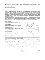
2. The fault-tolerant flight controller scheme
The logical scheme of the full fault-tolerant flight controller is reported in Fig. 1. The picture
shows four main elements, the autopilot (A/P), the actuators health monitor, the Stability
and Controllability Augmentation System (SCAS), based on the DAMF, and the Control
Allocation module. The last two elements represent the Fault-Tolerant Control System
(FTCS) that is the object of this chapter.


Fig. 1. The first layer scheme of the full Flight Control System
Although adaptive control exhibits great reconfiguration capabilities, in case of in-flight
faults, abrupt and dramatic changes in control effectiveness and/or plant dynamics may
occur, such that the adaptive controller may not be able to recover the vehicle. Therefore, an
adaptive controller could take advantage of a control allocation module to ensure the
generation of the demanded moments by the optimal control system, both in healthy and
faulty conditions of the actuation system.
The remaining two elements are not the focus of this work and they are developed with
classic techniques. In details, the A/P is designed by means of the classic sequential loop
closures, implementing the typical guidance modes for the aircraft (see Table. 1).

Longitudinal Lateral
Altitude Hold/Select Heading Hold/Select
GlideSlope Intercept Localizer Intercept
Approach Lon Approach Lat

Table 1. List of Autopilot modes
Fault-Tolerance of a Transport Aircraft with Adaptive Control and Optimal Command Allocation

161
Also the health monitoring of actuators is a very trivial system based on the comparison
between the input and the output of each actuators. In the numerical validation it is
supposed to use a monitoring system with the capability to detect an actuator fault within
10 seconds, and to pass the binary information healthy/faulty to the control allocation
system. In the following two sections the elements of the FTCS are briefly recalled.
3. Adaptive control system
The core module of the whole flight control system is the SCAS that is in charge of
guaranteeing vehicle attitude control and stability. As already said, the proposed algorithm
for this module has been designed using a Direct Adaptive Model-Following method
(Boskovic & Mehra, 2002; Kim et al., 2003; Tandale & Valasek, 2003), having the advantage
of strong robustness against model parameter uncertainty, and a good capability of reacting
to system parameters’ variation. Moreover, the model following strategy lets the designer to
define in a clear and simple way the reference dynamics for the system, thus making this
control strategy very attractive among other available robust control techniques. In the
following some recalls about the DAMF are given.
3.1 Theoretical recalls
DAMF is a Model Reference Control Strategies and it earns its robustness properties by
means of a direct adaptation of control loop gains to asymptotically reach two objectives.
The first is a null error between the output of the reference model and the one of real plant.
The second objective is to minimize the control effort. As already said, the proposed
adaptation algorithm is based on the Lyapunov theory. A mathematical description of the
method, fully reported in (Kim et al., 2003), follows. Let us consider the linear model of a
plant:

Cxy
dBuAxx

=
++=

(1)
with x ∈ ℜ
n
the state vector, y ∈ ℜ
l
the output vector, u ∈ ℜ
m
the control vector, A ∈ ℜ
nxn
,
B ∈ ℜ
nxm
, C ∈ ℜ
lxn
and the term d represents the trim data. The reference system dynamics is
written in term of desired input-output behaviour:

rByAy
mmmm
+
=

(2)
where y
m
is the desired output for the plant, r is the given demand, A
m

and B
m
represent the
reference linear system. The control laws structure is defined as follows:

(
)
m
yKrxGCu
000
+
+
+
=
ν
(3)
where G
0
, C
0
and v are proper terms generated by the adaptation rules, instead K
0
is a feed-
forward gain matrix off-line computed. It is now possible to calculate the error function as
follows:

m
yye
−
=

(4)
and to evaluate the error dynamics, in terms of the plant parameters and the reference
system dynamics:
Advances in Flight Control Systems

162

()
rByACdyKCBCCBCrCBCxGCBCCAe
mmmm
−
−
+
+
+
+
+
=
000000
ν

(5)
Assuming a desired error system dynamics, expressed as:

Φ
+
=
eAe
e


(6)
where A
e
is a stable and properly chosen matrix, and Φ represents a bounded forcing
function, it is possible to write the following identities:

em
m
e
AAKCBC
CdCBC
BCBC
CAGCBCCA
−=
−=
=
=+
0
*
0
**
0
*
0
*
0
*
0
ν
(7)

Equations 7 allow to write the expressions of the optimal terms G
0
*
, C
0
*
, v
*
and K
0
to obtain a
perfect model inversion that guarantees the asymptotical stability of the closed loop system
and the asymptotical null error.

(
)
()
()
emm
m
m
em
AABK
CdB
BCBC
CACABG
−=
−=
=
−=

−
−
−
−
1
0
1*
1
*
0
1*
0
ν
(8)
In order to evaluate the left hand terms (the gains of the controller), Equations 8 require
matrix B
m
to be invertible and CB matrix to be pseudo-invertible. While the former is a
design parameter, the latter, called high frequency gain, is a structural characteristic of the
plant. Anyway, modern aircrafts have typically a sufficient redundancy order for the control
surfaces, thus ensuring not to lose rank order even in the case of single and often double
actuators failure. Concerning the C matrix, no sensor failure cases are addressed in this
chapter, anyway the device redundancy or several techniques, available in literature (f.i.
Kalman filtering), may ensure a full state feedback, even though each signal may lose
accuracy in case of sensor failure.
It should be anyway noted that the control parameters of Equation 8 do not take into
account the system parameters variation. However, the system parameters uncertainties can
be modelled by a proper variation of the matrices in Equation 1. Finally, a set of adaptation
rules is necessary to react to the system parameters variation and uncertainty, Lyapunov
theory furnishes a very efficient solution. First of all, let us define the differences between

the actual adaptive parameters and the optimal ones:

*
00
1
0
1*
0
*
00
ννν
−=Δ
−=ΔΨ
−=Δ
−−
CC
GGG
(9)
After some manipulations (Kim et al., 2003), here left out for the sake of brevity, it is now
possible to write the real expression of the error dynamics taking into account a parameters
variation:
Fault-Tolerance of a Transport Aircraft with Adaptive Control and Optimal Command Allocation

163

ν
Δ
+
⋅
Δ

Ψ
+
⋅
Δ
+
=
mmme
BuBxGBeAe

(10)
It is allowed to impose the Lyapunov stability condition for the error system. So, let us
consider the Lyapunov candidate function:

321
γ
νν
γγ
ΔΔ
+
⎭
⎬
⎫
⎩
⎨
⎧
ΔΨΔΨ
+
⎭
⎬
⎫

⎩
⎨
⎧
ΔΔ
+=
TTT
T
tr
GG
trPeeV
(11)
where P is the matrix solution of Lyapunov equation:

QPAPA
e
T
e
−=+
(12)
with Q is a positive definite weighting matrix. By calculating the time derivative of the
Lyapunov candidate function and by casting it to get null, the following conditions can be
found, that represent the adaptation rules for the control laws parameters.

PeB
CPeuBCC
PexBG
T
m
TT
TT

m
m
30
0020
10
γν
γ
γ
−=
−=
−=



(13)
Moreover by taking into account the Equations 10, 11 and 13 it is possible to demonstrate
the non-positiveness of Lyapunov candidate function derivative:

0≤−= PeeV
T

(14)
which assures the asymptotical stability for the error dynamic system.
3.2 Implementation of the SCAS module
The SCAS module is made of two nested sub-modules, taking advantage of the dynamics
separation principle, being the angular rate dynamics sufficiently faster than those of the
attitude ones. This two modules architecture also leads to a relevant reduction of the overall
complexity (in terms of states number) of the adaptive algorithm. The detailed structure of
each Multi Input Multi Output (MIMO) controller is reported in Fig. 2. The design of both
inner and outer loops consists in tuning some parameters. First of all, the matrices A

m
and
B
m
, representing the dynamics of the Reference Model, must be selected with the limitation
that the former must trivially be chosen with negative eigenvalues and the latter must be
chosen invertible. These two matrices actually define the control system performance
requirements. For both attitude and rates regulators, a couple of very simple reference
models made of two diagonal systems (1
st
order and decoupled systems) have been chosen.
The desired error dynamics are chosen through the matrix A
e
by which, it is also possible to
modify the system capability to reject noise and disturbances.
The matrix Q, used in the Equation 12 for the calculation of P, has the meaning of a
weighting matrix. By fine tuning this matrix, it is possible to give more or less relevance to
the tracking requirement of one or more output variables with respect to the others. Finally,
the three parameters
γ
1
,
γ
2
and
γ
3
(evaluated by means of a trial and error procedure) are used
to regulate the adaptive capability. As a reminder, in Table 2 all the design parameters are
reported.

Advances in Flight Control Systems

164

Fig. 2. SCAS sub-module logical architecture


A
m
, B
m
A
e
Q
γ
1
, γ
2
, γ
3

Inner
Loops
⎥
⎥
⎥
⎦
⎤
⎢
⎢

⎢
⎣
⎡
⎥
⎥
⎥
⎦
⎤
⎢
⎢
⎢
⎣
⎡
−
−
−
100
010
001
,
100
010
001

⎥
⎥
⎥
⎦
⎤
⎢

⎢
⎢
⎣
⎡
−
−
−
5.400
05.40
005.4

⎥
⎥
⎥
⎦
⎤
⎢
⎢
⎢
⎣
⎡
100
02.10
008.0

⎥
⎥
⎥
⎦
⎤

⎢
⎢
⎢
⎣
⎡
1.0
1.0
06.0

Outer
Loops
⎥
⎦
⎤
⎢
⎣
⎡
⎥
⎦
⎤
⎢
⎣
⎡
−
−
5.00
05.0
,
5.00
05.0

⎥
⎦
⎤
⎢
⎣
⎡
−
−
75.00
05.1

⎥
⎦
⎤
⎢
⎣
⎡
5.00
01

⎥
⎥
⎥
⎦
⎤
⎢
⎢
⎢
⎣

⎡
2.0
01.0
01.0

Table 2. SCAS module parameters
4. The control allocation module
As mentioned in the introduction a control allocation algorithm can be very useful for
control reconfiguration purposes due to its ability of managing actuator redundancy, so to
redistribute control effort after a failure event. Moreover, it may be a great support for an
optimal control strategy, such as the DAMF that works well in the case of limited faults (i.e.
the plant dynamics do not change dramatically) and in any case it does not take into account
the limited range and limited rate of the control variables.
4.1 Theoretical background
In this section the control allocation problem is briefly introduced. Given a control vector
u
p
∈ ℜ
m
as computed by the control system (see Equation 3), a desired moment vector
v
des
∈ ℜ
l
can be defined as:

pdes
CBuv
=
(15)

where the matrix product CB is the high frequency gain of the healthy system (no faults). In
the event of one or more faults, system defined in Equation 1 becomes:
Fault-Tolerance of a Transport Aircraft with Adaptive Control and Optimal Command Allocation

165

Cxy
dBuuBAxx
lockfault
=
+++=

(16)
where B
fault
is the control matrix of the failed plant which can be expressed as:

Π
=
BB
fault
(17)
where Π is a diagonal matrix with the elements π
i
= 0 for i-th actuator failed and π
i
= 1 for a
healthy actuator. This matrix accounts for the fact that failed actuators cannot be used
anymore to change the system’s dynamics. The term Bu
lock

accounts for a residual moment
due to an actuator locked in a fixed position, so we set u
lock
(j) = 0 if j-th actuator is healthy
and u
lock
(j) = u
j
if j-th actuator is locked at u
j
. After this setting, the residual moment to be
attained by the failed system is defined as

lockdes
CBuvv
−
=
Δ
(18)
which is the moment to be attained with the failed high frequency gain matrix B
fault
.
Therefore the goal of control allocation is to find a control ū ∈ ℜ
m
such that CB
fault
ū =Δv. The
new control vector shall also satisfy the constraints on maximum and minimum values,
which can be computed at each instant depending on the actual position and rate limits, that
is, u

min
≤
ū
≤
u
max
.
Generally speaking a solution to the above problem may not exist or it may be not unique
depending on the rank of matrix CB
fault
. If there are more solutions, the exceeding control
authority can be exploited to choose the solution which is the nearest to a reference control
vector u
p
∈ ℜ
m
(for example the one computed by the control system). A common approach
to solve the control allocation problem is based on the following weighted least square
formulation (Harkegard, 2002):

(
)
(
)
22
maxmin
min vuCBWuuWu
faultvpu
uuu
w

Δ−+−=
≤≤
γ
(19)
where ║·║
2
is the L
2
-norm, u
p
is a reference control vector, W
u
and W
v
are non-singular
weighting matrices. The first term of the above minimization problem allows to choose,
among all the feasible control vectors which minimize the L
2
-norm of the error CB
fault
u-Δv,
the one minimizing the norm of (u-u
p
). The weighting factor
γ
defines the relative degree of
importance between the moments error CB
fault
u-Δv and the control error (u-u
p

). Obviously
γ

should be chosen large enough to ensure the minimization of the error in attaining the
desired moments.
In this chapter we will address the problem of control allocation with the use of a technique
based on the active set method and described in (Harkegard, 2002). Active set methods are
very common in constrained quadratic programming. They only consider active constraints
(equality constraints) and disregard inactive constraints. Therefore active set algorithms
move on the surface defined by the set of the active constraints (named Working Set) to get
an improved solution. The working set is continuously updated during the execution of the
algorithm. In fact, whenever a new constraint is violated, it is added to the current working
set. On the other hand, if a feasible solution has been found by the algorithm, but a
Lagrange multiplier related to the current working set is negative, the corresponding active
constraint is dropped in order to get an improved solution. An exhaustive description of the
Advances in Flight Control Systems

166
control allocation algorithm used in this chapter can be found in (Harkegard, 2002). Some
recalls are given in the section below.
4.2 Control allocation algorithm
For each iteration step of the algorithm the following optimization problem is solved:

(
)
⎟
⎟
⎠
⎞
⎜

⎜
⎝
⎛
=
⎟
⎟
⎠
⎞
⎜
⎜
⎝
⎛
=∈=
−+
pu
v
u
v
ki
k
p
uW
vW
b
W
BW
AWip
bupA
γ
γ

, , ,0
;min
2
(20)
where u
k
is the starting solution at the iteration step k, the set W
k
is the current working set,
that is, the set containing the active constraints (i.e. saturated controls) which are expressed
through the equality p
i
=0, while the remaining inequality constraints are disregarded.
Solution to the least square problem of Equation 21 consists of finding the optimal
perturbation p which can be obtained by using a simple pseudo inversion method
(Harkegard, 2002). Once the constraints on actuator limits have been set

⎟
⎟
⎠
⎞
⎜
⎜
⎝
⎛
−
+
=
⎟
⎟

⎠
⎞
⎜
⎜
⎝
⎛
−
+
=
≥
min
max
,
;
u
u
U
I
I
C
UCu
(21)
(I
mxm
is the identity matrix), if the solution u
k
+p is feasible, the Lagrange multipliers
λ
i

associated with the active constraints are computed. If they are non-negative, the optimum
solution is obtained otherwise the i-th constraint is dropped from the active set because a
better solution can be found according to the meaning of Lagrange multipliers (Luenberger,
1989). In the case that u
k
+p is not feasible, the maximum step α is calculated such that u
k
+
α
p
is still feasible and a new constraint is added to the working set. This iterative procedure is
then repeated until a suitable solution and a working set with negative related Lagrange
multiplier are found.
4.3 Remarks
As above described control allocation algorithm has the aim of redistribute the control effort
among the “healthy” surfaces to achieve the moments needed to keep the system along
reference trajectory. In view of these considerations we argue that control allocation can be
very useful, when used in conjunction with a direct adaptive control in those critical failure
scenarios which can be hardly handled by the only use of the adaptive controller.
Nevertheless, in order to be effective for reconfiguration purposes, control allocation needs a
Fault Detection (FD) system, which gives information about the health of the surfaces’
actuators. This aspect could make unfeasible the use of a CA scheme. Anyway, in the
following sections it will be shown that, in order to obtain a satisfactory performance of the
CA module, only limited failure information are needed. In fact, also a very simple
monitoring algorithm, based on the actuator model and on the surface actual position, can
be sufficient to establish whether an actuator is failed or not. The results show that the use of
a CA scheme allows significant improvements of the control system performances also in
the event of very critical failures and it only needs limited information about actuators’