Parallel Manipulators Towards New Applications Part 1 pdf

Parallel Manipulators
Tow a rds N e w Ap pli c ations

Parallel Manipulators
Tow a rds N e w Ap pli c ations



Edited by
Huapeng Wu

I-Tech











Published by I-Tech Education and Publishing

I-Tech Education and Publishing
Vienna
Austria


Abstracting and non-profit use of the material is permitted with credit to the source. Statements and
opinions expressed in the chapters are these of the individual contributors and not necessarily those of
the editors or publisher. No responsibility is accepted for the accuracy of information contained in the
published articles. Publisher assumes no responsibility liability for any damage or injury to persons or
property arising out of the use of any materials, instructions, methods or ideas contained inside. After
this work has been published by the I-Tech Education and Publishing, authors have the right to repub-
lish it, in whole or part, in any publication of which they are an author or editor, and the make other
personal use of the work.

© 2008 I-Tech Education and Publishing
www.i-techonline.com

Additional copies can be obtained from:


First published April 2008
Printed in Croatia



A catalogue record for this book is available from the Austrian Library.
Parallel Manipulators, Towards New Applications, Edited by Huapeng Wu
p. cm.
ISBN 978-3-902613-40-0
1. Parallel Manipulators. 2. New Applications. I. Huapeng Wu





V


Preface



In recent years, parallel kinematics mechanisms have attracted a lot of attention from the
academic and industrial communities due to potential applications not only as robot ma-
nipulators but also as machine tools. Generally, the criteria used to compare the perform-
ance of traditional serial robots and parallel robots are the workspace, the ratio between the
payload and the robot mass, accuracy, and dynamic behaviour. In addition to the reduced

coupling effect between joints, parallel robots bring the benefits of much higher payload-
robot mass ratios, superior accuracy and greater stiffness; qualities which lead to better dy-
namic performance. The main drawback with parallel robots is the relatively small work-
space.
A great deal of research on parallel robots has been carried out worldwide, and a large
number of parallel mechanism systems have been built for various applications, such as re-
mote handling, machine tools, medical robots, simulators, micro-robots, and humanoid ro-
bots.
This book opens a window to exceptional research and development work on parallel
mechanisms contributed by authors from around the world. Through this window the
reader can get a good view of current parallel robot research and applications.
The book consists of 23 chapters introducing both basic research and advanced develop-
ments. Topics covered include kinematics, dynamic analysis, accuracy, optimization design,
modelling, simulation and control of parallel robots, and the development of parallel
mechanisms for special applications. The new algorithms and methods presented by the
contributors are very effective approaches to solving general problems in design and analy-
sis of parallel robots.
The goal of the book is to present good examples of parallel kinematics mechanisms and
thereby, we hope, provide useful information to readers interested in building parallel ro-
bots.


Editor


Huapeng Wu
Institute of Mechatronics and Virtual Engineering
Lappeenranta University of Technology
Finland

VII





Contents




Preface
V


1. Control of Cable Robots for Construction Applications 001
Alan Lytle, Fred Proctor and Kamel Saidi


2. Dynamic Parameter Identification for Parallel Manipulators 021
Vicente Mata, Nidal Farhat, Miguel Díaz-Rodríguez,
Ángel Valera and Álvaro Page



3. Quantifying and Optimizing Failure Tolerance of a Class of Parallel Manipu-

lators
045
Chinmay S. Ukidve, John E. McInroy and Farhad Jafari


4. Dynamic Model of a 6-dof Parallel Manipulator Using the Generalized
Momentum Approach
069
António M. Lopes and Fernando Almeida

5. Redundant Actuation of Parallel Manipulators 087
Andreas Müller


6. Wrench Capabilities of Planar Parallel Manipulators and their Effects Under
Redundancy
109
Flavio Firmani, Scott B. Nokleby, Ronald P. Podhorodeski and Alp Zibil


7. Robust, Fast and Accurate Solution of the Direct Position Analysis of
Parallel Manipulators by Using Extra-Sensors
133
Rocco Vertechy and Vincenzo Parenti-Castelli


8. Kinematic Modeling, Linearization and First-Order Error Analysis 155
Andreas Pott and Manfred Hiller

9. Certified Solving and Synthesis on Modeling of the Kinematics. Problems
of Gough-Type Parallel Manipulators with an Exact Algebraic Method
175
Luc Rolland

10. Advanced Synthesis of the DELTA Parallel Robot for a Specified Works-
pace
207
M.A. Laribi, L. Romdhane and S. Zeghloul


VIII
11. Size-adapted Parallel and Hybrid Parallel Robots for Sensor Guided Micro
Assembly
225
Kerstin Schöttler, Annika Raatz and Jürgen Hesselbach


12. Dynamics of Hexapods with Fixed-Length Legs 245
Rosario Sinatra and Fengfeng Xi


13. Cartesian Parallel Manipulator Modeling, Control and Simulation 269
Ayssam Elkady, Galal Elkobrosy, Sarwat Hanna and Tarek Sobh


14. Optimal Design of Parallel Kinematics Machines with 2 Degrees of Free-
dom
295
Sergiu-Dan Stan, Vistrian Maties and Radu Balan

15. The Analysis and Application of Parallel Manipulator for Active Reflector
of FAST
321
Xiao-qiang Tang and Peng Huang


16. A Reconfigurable Mobile Robots System Based on Parallel Mechanism 347
Wei Wang, Houxiang Zhang, Guanghua Zong and Zhicheng Deng


17. Hybrid Parallel Robot for the Assembling of ITER 363
Huapeng Wu, Heikki Handroos and Pekka Pessi


18. Architecture Design and Optimization of an On-the-Fly Reconfigurable
Parallel Robot
379
Allan Daniel Finistauri, Fengfeng (Jeff) Xi and Brian Petz


19. A Novel 4-DOF Parallel Manipulator H4 405
Jinbo Wu and Zhouping Yin


20. Human Hand as a Parallel Manipulator 449
Vladimir M. Zatsiorsky ad Mark L. Latash

21. Mobility of Spatial Parallel Manipulators 467
Jing-Shan Zhao, Fulei Chu and Zhi-Jing Feng


22. Feasible Human-Spine Motion Simulators Based on Parallel Manipulators 497
Si-Jun Zhu, Zhen Huang and Ming-Yang Zhao





1
Control of Cable Robots for
Construction Applications
Alan Lytle, Fred Proctor and Kamel Saidi
National Institute of Standards and Technology
United States of America
1. Introduction
The Construction Metrology and Automation Group at the National Institute of Standards
and Technology (NIST) is conducting research to provide standards, methodologies, and
performance metrics that will assist the development of advanced systems to automate
construction tasks. This research includes crane automation, advanced site metrology
systems, laser-based 3D imaging, calibrated camera networks, construction object
identification and tracking, and sensor integration and process control from Building
Information Models. The NIST RoboCrane has factored into much of this research both as a
robotics test platform and a sensor/target positioning apparatus. This chapter provides a
brief review of the RoboCrane platform, an explanation of control algorithms including the
NIST GoMotion controller, and a discussion of crane task decomposition using the Four
Dimensional/Real-time Control System approach.
1.1 The NIST RoboCrane

RoboCrane was first developed by the NIST Manufacturing Engineering Laboratory’s
(MEL) Intelligent Systems Division (ISD) in the late 1980s as part of a Defense Advanced
Research Project Agency (DARPA) contract to stabilize crane loads (Albus et al., 1992). The
basic RoboCrane is a parallel kinematic machine actuated through a cable support system.
The suspended moveable platform is kinematically constrained by maintaining tension due
to gravity in all six support cables. The support cables terminate in pairs at three vertices
attached to an overhead support. This arrangement provides enhanced load stability over
beyond traditional lift systems and improved control of the position and orientation (pose)
of the load. The suspended moveable platform and the overhead support typically form two
opposing equilateral triangles, and are often referred to as the “lower triangle” and “upper
triangle,” respectively.
The version of RoboCrane used in this research is the Tetrahedral Robotic Apparatus
(TETRA). In the TETRA configuration, all winches, amplifiers, and motor controllers are
located on the moveable platform as opposed to the support structure. The upper triangle
only provides the three tie points for the cables, allowing the device to be retrofitted to
existing overhead lift mechanisms. Although the TETRA configuration is presented in this
chapter, the control algorithms and the Four Dimensional/Real-time Control System
(4D/RCS), for 3D + time/Real-time Control System, task decomposition are adaptable to
Parallel Manipulators, Towards New Applications

2
many different crane configurations. The functional RoboCrane design can be extended and
adapted for specialized applications including manufacturing, construction, hazardous
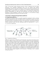
waste remediation, aircraft paint stripping, and shipbuilding. Figure 1 depicts the
RoboCrane TETRA configuration (a) and the representative work volume (b). Figure 2
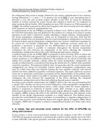
shows additional retrofit configurations of the RoboCrane platform, and Figure 3 shows
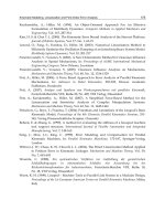
implementations for shipbuilding (Bostelman et al., 2002) and aircraft maintenance.


(a) (b)

Fig. 1. RoboCrane – TETRA configuration (a); Rendering of the RoboCrane environment.
The shaded cylinder represents the nominal work volume (b).

Fig. 2. Illustrations of RoboCrane in possible retrofitted configurations: Tower Crane (top),
Boom Crane (lower left) and Gantry Bridge Crane (lower right).
1.2 Motivation for current research
Productivity gains in the U.S. construction sector have not kept pace with other industrial
sectors such as manufacturing and transportation. These other industries have realized their
productivity advances primarily through the integration of information, communication,
Control of Cable Robots for Construction Applications

3
automation, and sensing technologies. The U.S. construction industry lags these other
sectors in developing and adopting these critical, productivity-enhancing technologies.
Leading industry groups, such as the Construction Industry Institute (CII), Construction
Users Roundtable (CURT) and FIATECH, have identified the critical need for fully
integrating and automating construction processes.
Robust field-automation on dynamic and cluttered construction sites will require advanced
capabilities in construction equipment automation, site metrology, 3D imaging, construction
object identification and tracking, data exchange, site status visualization, and design data
integration for autonomous system behavior planning. The NIST Construction Metrology
and Automation Group (CMAG) is conducting research to provide standards,
methodologies, and performance metrics that will assist the development, integration, and
evaluation of these technologies. Of particular interest are new technologies and capabilities
for automated placement of construction components.



(a) (b)
Fig. 3. The NIST Flying Carpet – a platform for ship access in drydocks (a) and the NIST

Aircraft Maintenance Project (AMP) – a platform for aircraft access in hangars (b).
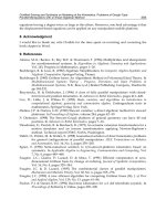
2. RoboCrane kinematics
From (Albus et al., 1992), given an initial condition where the overhead support and the
suspended platforms are represented by parallel, equilateral triangles with centers aligned
along the vertical axis Z, (see Figure 4), the positions of the upper triangle with vertices A, B,
and C and lower triangle with vertices D, E, and F are expressed as

0
112
333
333
0
211
333
333
000
bb
bbb
hhh
aa
aaa
−
⎡
⎤⎡ ⎤⎡⎤
⎢
⎥⎢ ⎥⎢⎥
⎢
⎥⎢ ⎥⎢⎥
=− =− =
⎢

⎥⎢ ⎥⎢⎥
⎢
⎥⎢ ⎥⎢⎥
−−−
⎣
⎦⎣ ⎦⎣⎦
−
⎡
⎤⎡⎤⎡⎤
⎢
⎥⎢⎥⎢⎥
⎢
⎥⎢⎥⎢⎥
=− = =
⎢
⎥⎢⎥⎢⎥
⎢
⎥⎢⎥⎢⎥
⎣
⎦⎣⎦⎣⎦
ABC
DEF
(1)
Parallel Manipulators, Towards New Applications

4
With the positions of the vertices of triangles ABC and DEF as described in equations (1),
when the lower platform is moved to a new position and orientation (D´E´F´) through a
translation of

x
y
z
u
u
u
⎡
⎤
⎢
⎥
=
⎢
⎥
⎢
⎥
⎣
⎦
U
(2)
and a rotation of
(,,) () () ()
yxz z x y
RRRR
γ
θφ φ θ γ
=
⋅⋅ (3)
the cable lengths can be expressed as

12 12

22 22
32 32
11 12
21 22
31 32
22
33
33
12 12
33 33
33 33
22
33
33
1
3
3
11
33
33
1
3
3
xx
yy
zz
x
y
z
baQ u baQ u

baQu baQu
haQ u haQ u
baQ aQ u
baQaQ u
haQ aQ u
⎡⎤⎡⎤
−+ − −+ −
⎢⎥⎢⎥
⎢⎥⎢⎥
⎢⎥⎢⎥
=− + − =− + −
⎢⎥⎢⎥
⎢⎥⎢⎥
⎢⎥⎢⎥
−+ − −+ −
⎢⎥⎢⎥
⎣⎦⎣⎦
⎡⎤
−− −
⎢⎥
⎢⎥
⎢⎥
=− − − −
⎢⎥
⎢
⎢
−− − −
⎢
⎣⎦
12

3
LL
L
11 12
21 22
31 32
11 12 11 12
21 22 21 22
31 32 3
1
3
3
21
33
33
1
3
3
11
33
33
21 11
33 33
33 33
1
3
3
x
y
z

xx
yy
z
aQ aQ u
baQaQ u
haQ aQ u
aQ aQ u b aQ aQ u
baQaQ u baQaQ u
haQ aQ u haQ
⎡
⎤
−− −
⎢
⎥
⎢
⎥
⎢
⎥
=−− −
⎢
⎥
⎥
⎢⎥
⎥
⎢⎥
−− − −
⎥
⎢⎥
⎣
⎦

⎡⎤
−− −+−−
⎢⎥
⎢⎥
⎢⎥
=+− − =−+− −
⎢⎥
⎢⎥
⎢⎥
−+ − − −+
⎢⎥
⎣⎦
4
56
L
LL
132
1
3
3
z
aQ u
⎡
⎤
⎢
⎥
⎢
⎥
⎢
⎥

⎢
⎥
⎢
⎥
⎢
⎥
−−
⎢
⎥
⎣
⎦
(4)
where



′
′′
===
′
′′
===
123
456
LADLBDLBE
LCELCFLAF
(5)
and
ij
Q represents an element in the following rotation matrix:

cos( )cos( ) sin( )sin( )sin( ) cos( )sin( ) sin( )cos( ) cos( )sin( )sin( )
cos( )sin( ) sin( )sin( ) cos( ) cos( ) cos( ) sin( )sin( ) cos( )sin( ) cos( )
sin( )cos( ) sin( ) cos( ) cos( )
γ
φ γθφ θφ γ φ γθφ
γ
φ γθφ θφ γφ γθφ
γθ θ γθ
−− +
⎡ ⎤
⎢ ⎥
=− −
⎢ ⎥
⎢ ⎥
−
⎣ ⎦
Q
(6)
Therefore, for any new desired pose of the moving platform described by equations (2) and
(3), the required cable lengths to achieve that pose can be calculated by the inverse
kinematic equations shown in equations (4).
Control of Cable Robots for Construction Applications

5

Fig. 4. Graphical representation of the RoboCrane cable support structure.
3. Measuring RoboCrane pose
The controller's estimate of the actual pose of RoboCrane differs from the actual pose due to
several sources of error. Position feedback is provided through motor encoders that measure

rotational position. Cable length is computed by multiplying the rotational position by the
winch drum radius, with a suitable scale factor and offset.
However, the winch drum radius is not constant, but varies depending on the amount of
cable that has already been wrapped around the drum, increasing its radius. It is possible to
keep track of this and change the radius continually, by building a table that relates motor
rotational position with effective radius.
Another source of error is that the cable length is affected by sag due to gravity. This sag
depends on the pose of the platform and its load. Compensation can be achieved using an
iterative process that begins with the nominal cable lengths, computes the platform pose
using the forward kinematics equations, and determines the tensions on each of the cables
using the transpose of the Jacobian matrix and the weight of the platform. The tensions can
be used to generate the actual catenary curve of the cable, taking its nominal length as the
Parallel Manipulators, Towards New Applications

6
length of the hanging catenary curve. This process is repeated iteratively, with the nominal
cable length as the fixed arc length of the catenary, and the chord between its endpoints as
the continually revised length used by the forward kinematics.
Calibration errors in the mounting points of the ends of the cables further contribute to pose
error. In practice these are not fixed points, but vary as the angles of the cables change the
contact point to the pulleys or eye bolts that affix the ends. Even if these contact points were
constant, their actual locations can be difficult to measure with precision, given their large
displacement over a typical work volume.
Given these many sources of error, it is desirable to be able to measure the pose of the
platform directly. There are many commercial systems for this purpose. An initial approach
to external measurement implemented on RoboCrane uses a laser-based, large-scale, site
measurement system (SMS).
3.1 The site measurement system (SMS)
A laser-based site measurement system (SMS) is used to track RoboCrane’s pose and to
measure object locations within the work volume. The SMS uses stationary, active-beacon

laser transmitters and mobile receivers to provide millimeter-level position data at an
update rate of approximately 20 Hz. This technology was chosen based upon a combination
of factors including indoor/outdoor operation, accuracy, update-rate, and support for
multiple receivers.
Each SMS transmitter emits two rotating, fanned laser beams and a timing pulse. Elevation
is calculated from the time difference between fanned beam strikes. Azimuth is referenced
from the timing pulse. The field of view of each transmitter is approximately 290° in
azimuth and ± 30° in elevation/declination.
Similar to GPS, the SMS does not restrict the number of receivers. Line-of-sight to at least
two transmitters must be maintained by each receiver in order to calculate that receiver’s
position. The optical receivers each track up to four transmitters and wirelessly transmit
timing information to a base computer for position calculation.
For tracking RoboCrane’s pose, four laser transmitters are positioned and calibrated on the
work volume perimeter, and three SMS receivers are mounted on RoboCrane near the
vertices of the lower triangle. The receiver locations are registered to the manipulator during
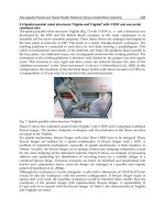
an initial setup process in the local SMS coordinate frame. A transmitter and an optical
receiver are shown in Figure 5. The SMS receivers mounted on RoboCrane are shown in
Figure 6.



(a) (b)
Fig. 5. An SMS laser transmitter (a) and an SMS optical receiver (b).
Control of Cable Robots for Construction Applications

7
The drawback of these systems is the added cost, and the need to maintain lines-of-sight
between the platform and transmitters, potentially interfering with intended use. The
benefits of accurate pose measurement are often significant enough to warrant their use.
In the first implementation of the SMS to track RoboCrane, position estimates were obtained

at several stopping points during RoboCrane’s trajectory, and these estimates were used as
coarse correction factors for the encoder positions. Current work is focused on a dynamic
tracking approach to eliminate the need for stopping points.


Fig. 6. The SMS on RoboCrane showing a close-up view of one of the three receivers.
3.2 Dynamic pose measurement
A commanded pose will generally result in a different actual pose due to various sources of
system error such as those discussed previously. This relationship is depicted as

→→NXA (7)
or, in matrix form,

=
NX A (8)
where
N is the commanded pose, X is the perturbation that includes all the sources of
error, and
A is the actual pose that results. The effects of X can be cancelled by
commanding an adjusted pose,
∗
N , where

∗
=
-1
NNX (9)
Using the adjusted pose allows us to achieve the original desired pose since

∗

=
NX N
(10)
In general, most of the sources of error are unknown and variable, so computing
-1
X apriori
is not feasible. However,
-1
X can be estimated by comparing a previously commanded
Parallel Manipulators, Towards New Applications

8
adjusted pose,
∗
N
, with the resulting actual pose,
∗
A , as measured by the SMS. For time
step, (i-1)

**
11 1
ii i
−
−−
=NX A (11)
And the inverse of
1i
−
X can be calculated as

(
)
(
)
1
**
111iii
−
−
−−
=
-1
XAN (12)
For the current time step, (i), the commanded adjusted pose can be calculated as

(
)
*
1iii−
=
-1
NNX
(13)
where
i
N is the desired pose for the current time step and
1i
−
X is the perturbation from the

previous time step. Therefore,

*
ii i
≈NX N (14)
If the platform is moving, then the cancellation is not perfect, since we are trying to cancel
this time step's unknown perturbation transform with the inverse from the previous time
step, which will be slightly different. If the platform is stationary, the two converge and the
cancellation becomes perfect.
Platform motion has a more pronounced practical effect due to measurement latency for
A .
When computing
-1
X , it is important that the N and
A
poses are synchronized. If the
measured
A
pose lags the nominal N pose, then the compensation will have the effect of
leading the motion. When speed slows, this leading will become an overshoot, and the
platform will oscillate.
In the presence of measurement latency, one solution is to only compute the compensating
transform
-1
X when the platform is stationary. With this method, the platform is moved into
an area of interest, held stationary for at least the latency period, and
-1
X is computed. From
that point, iteration is suppressed, and the compensating transform is constant. As the
platform moves away from the compensation point, its accuracy diminishes.

If the latency is constant and can be measured, a solution is to keep a time history of
nominal poses and their associated inverse transforms, and look back into this history by the
amount of latency to associate a pair
N and
-1
X to the latent A measurement. If the
measurements can be timestamped, then the same technique can be supplemented with
timestamps to make the association. This technique can be used in the presence of variable
measurement latency.
Controller latency also has an effect on the accuracy of the compensating transform. Figure 7
shows the magnitude of the translation portion of the compensating transform during tests
with four different trajectory cycle times. In each test, the platform speed varied from
1 cm/s to 10 cm/s. These tests were done with a simulated measurement system that
simulates actual position from the servo position run through the forward kinematics. In
this case, the compensating transform should be small, and in fact it goes to zero as the
Control of Cable Robots for Construction Applications

9
motion pauses between each speed setting. It is apparent from these figures that as the
platform speed increases, the magnitude of the compensating transform increases, as is
expected from servo lag. It is also apparent that as cycle time increases, so does the
magnitude of the transform. This is due to the uncertainty between when nominal position
is registered by the controller, and when it is read out some fraction of a period later.




Fig. 7. Compensating transform magnitude (translation only) for four different trajectory
cycle times. As the trajectory cycle time increases, the magnitude increases, and becomes
more noisy as a result of the increased uncertainty in the latency between control output and

compensation. (Note: Figures intended as qualitative examples of cycle time effects.)
Whenever a new
-1
X transform is written to the controller, it has the potential to cause a
jump in motion. To prevent this, transforms are “walked in” according to speed and
acceleration limits. A large change in the transform will appear as a relatively quick but
controlled move to the new, more accurate position. The effect of compensation is illustrated
in Figure 8. The square path in the lower left of the figure is the uncompensated path, which
is offset and slightly skewed from the ideal path due to kinematic miscalibration. Shortly
after the second pass around the square path, compensation was turned on and its effects
walked in over several seconds. This interval appears as the two line segments connecting
the square paths. The square path in the upper right is the compensated path, whose
adherence to the nominal edges at 0 cm and 10 cm is quite good.
Parallel Manipulators, Towards New Applications

10

Fig. 8. Effect of in-process compensation The lower left square path is uncompensated and
differs due to kinematic miscalibration. The upper right path is compensated. The
connecting path results applying the compensation over time to avoid impulsive jumps.
When compensation is turned off, the last compensating transform remains in use. As the
platform moves away from the point at which this transform was calculated, the
compensation becomes less accurate. This is shown in Figure 9.


Fig. 9. Trajectory drift after cancelling in-process compensation. The correction was made at
location (0,0), and no further updates were performed.
4. RoboCrane control
4.1 GoMotion controller description
The RoboCrane controller is a two-level hierarchy. The bottom level is servo control, which

takes position setpoints for the cable lengths at a period of 1 millisecond, and runs a
proportional-integral-derivative (PID) controller using feedback from encoders mounted on
the motors to generate drive signals. The top level is trajectory planning, which takes
desired goal poses and plans smooth Cartesian motion along a linear path, taking into
account speed, acceleration and jerk constraints. The trajectory planner executes at a period
of 10 milliseconds, calculating intermediate poses that are run through the inverse kinematic
Control of Cable Robots for Construction Applications

11
equations to generate cable lengths sent to the servo controllers. Joint mode control is also
possible, with goals specified in terms of desired cable lengths. The inverse kinematics are
not needed in this case.
Servo control is divided among six similar modules, each running PID control with
extensions that handle velocity and acceleration feedforward terms, output biasing,
deadband and saturation detection for anti-windup of integral gain. A software application
programming interface (API) localizes how the servo modules connect to specific hardware
such as commercial input/output boards for encoder feedback and digital-to-analog
conversion, open-loop stepper motors or distributed input/output. The servo modules run
periodically at 10 times the period of the trajectory planner. Interpolation between setpoints
sent by the trajectory planner is done using either linear, cubic or quintic polynomial
interpolation of the setpoint over time, depending on application needs.
Trajectory planning is done following S-curve velocity profiling with specified velocity,
acceleration and jerk. S-curve profiling has the advantage of bounding jerk, when compared
with trapezoidal velocity profiling with abrupt changes in acceleration. S-curve profiling has
seven motion phases, as shown in Figure 10.


Fig. 10. S-curve velocity profile.
Here,
3

v ,
1
a and
0
j are the specific maximum velocity, acceleration and jerk, respectively. At
each trajectory time step, the distance increment is computed as the area under the S-curve
for that time interval.
In joint position control mode (individual cable actuation), trajectory planning is done for
each cable independently. Given a desired target cable length, the S-curve profile is
computed and distances are computed each trajectory period. These distances are sent to the
servo module for that joint for interpolation and tracking. Coordinated joint position control
is possible, in which a set of six target cable lengths comprises the goal. Six trajectory
profiles are computed, and five of the six are scaled so that their final arrival time matches
the time of the longest move.
In Cartesian position control mode, motion control is split into translation and rotation
vectors. The translation vector is a three-element vector with X, Y and Z components
pointing to the target location, with associated velocity, acceleration and jerk along the path.
The rotation vector is a three-element vector about which the overall rotation from the
current orientation to the target orientation takes place. The magnitude of this vector is the
amount of rotation. Angular velocity, acceleration and jerk are used to generate a profile for
this portion of the move. One of the two profiles is scaled to match the time of the longer of
the two so that the translation and rotation arrive at the same time. At each trajectory cycle,
Parallel Manipulators, Towards New Applications

12
the translation and rotation are computed, run through the inverse kinematics equations,
and sent as a set of target cable lengths for interpolation and tracking by the servo modules.
Motion along circular arcs is also supported. Rotational motion is planned as before.
Translational motion is planned along the arc, where the distance under the S-curve profile
is the distance along the arc. Aside from this geometric distinction, circular motion is the

same as linear motion.
4.2 Initialization
When the controller begins executing, it assumes that the cable length measurements are
uncalibrated. Cable length limits are invalid, as is any notion of the Cartesian pose of the
platform or its limits. The controller allows individual cables to be moved independently,
but inhibits Cartesian motion and cable length limit checking. Before any of these can take
place, the platform must be “homed” to establish the offset between the initial arbitrary
measurement of cable length (typically zero) and its true length.
In systems that lack a way to absolutely measure either cable lengths or Cartesian pose at
startup, a homing procedure is used. There are several variations in this method. In one,
fiducial marks are made on each cable, which when aligned with an associated mark on the
platform denote that the cable is at a known length. The operator must manually jog each
cable to align the marks, and indicate that the home condition has been met. The controller
then computes an offset that is added to the raw feedback from the motor encoder to yield
the known length value.
Another homing technique is to bring the platform to a known Cartesian location, such as
level and oriented properly atop a mark on the floor. This requires manually moving the
platform by adjusting cable lengths, which is unintuitive. In practice, the operator moves
each cable so that the platform is relatively close to the home location, and falsely indicates
that the cables are homed. Cartesian motion is then enabled, and the operator moves in
Cartesian space for the final alignment. During this falsely-homed period, the platform
motion will be skewed, but is usually close enough for intuitive positioning.
Homing is a time-consuming manual procedure. If the platform's Cartesian pose can be
measured directly, such as with the SMS, then homing is not necessary. In this case, the
controller is provided with the actual Cartesian position, which it runs through the inverse
kinematics to get the cable lengths. The difference between these computed cable lengths
and the uncalibrated lengths from the motor encoders is the offset used to calibrate the
feedback.
4.3 Control modes
The RoboCrane controller supports various control modes. Teleoperation allows an operator

to drive the platform directly, using a keyboard, mouse or joystick. Automatic control
allows the execution of scripted trajectories.
Teleoperated Control
: In teleoperated control, the operator uses a convenient input device,
such as a keyboard, mouse or joystick, to move the platform directly. Typically a joystick is
used, since it is most intuitive. This can be performed in either joint (i.e., cable lengths) or
Cartesian space. With cable lengths, the operator selects a cable, and shortens or lengthens
the cable according to the deflection of the joystick. If the controller has been homed, the
Cartesian position is continually updated using the forward kinematics. Cable length
motion is typically used only when homing the platform, since it results in unintuitive
platform motion.
Control of Cable Robots for Construction Applications

13
In Cartesian space, the operator uses the joystick to drive the platform in any of the X, Y and
Z directions, or to rotate about these directions. The controller supports two reference
frames: the world frame, with coordinates affixed to the unmoving ground; and the
platform (or tool) frame, with coordinates affixed to the moving platform. World mode is
typically used to position the platform near an area of interest, or to drive it along features
in the world, such as the floor or walls. Tool mode is used to position the platform by
driving it along axes aligned with grippers or tooling, so that approaches and departures
can be made along arbitrary directions. The controller supports the definition of arbitrary
tool coordinate systems, so that one tool can be dropped off, another picked up, and motion
with respect to the new tool axes can be accomplished.
In world mode, Cartesian speeds from the joystick are converted into cable speeds using the
inverse Jacobian. Given a desired Cartesian velocity of RoboCrane,
V , and using the inverse
Jacobian
1
matrix,

-1
J , the cable speed vector,

L , can be calculated as

=

-1
LJV (15)
where

L is the 6x1 cable speed matrix,
-1
J is the 6x6 inverse Jacobian transform matrix, and
V is the 6x1 Cartesian velocity vector (Tsai, 1999). The calculated cable speeds are
transformed into winch motor rotation rates that are sent to the winches. Each motor
encoder keeps track of the number of motor shaft revolutions and that number is directly
related to cable length. The six cable lengths are then used to calculate a new Jacobian
matrix, which is used the next time velocity commands are sent.
Since the inverse Jacobian matrix is calculated based on the instantaneous Cartesian pose of
RoboCrane, the initial pose of RoboCrane must be known. This initial pose can be calculated
by directly measuring the cable lengths and performing the forward kinematic calculations,
or by placing RoboCrane in a predefined home pose at the beginning of each teleoperation
session and initializing the cable lengths to preset values.
Speed changes are clamped to lie within acceleration limits, so that abrupt changes in
joystick position do not impart abrupt changes in motor speed. Cartesian position and
orientation limits are applied, so that attempts to drive the platform outside a limit will be
inhibited.
Automatic Control
: With automatic control, motions in either cable or Cartesian space can

be scripted in programs. These programs can be written by hand, or generated by off-line
programming systems that can automate the generation of complex tasks throughout a large
work volume. This is accomplished through a third level in the hierarchy, the Job Cell level.
This level interfaces to the motion controller using the same interface as the teleoperation
application, but sending discrete moves instead of teleoperation speeds.
There are two basic modes of automatic control, either in cable space or in Cartesian space.
Cable space motions are less common, and would be used to drive individual cables during
maintenance activities. Cartesian space motions are primarily used in applications. As with

1
The Jacobian transform (or simply Jacobian), J relates the velocities of the joints of a
manipulator to the velocities (translational and rotational) of its end-effector,


x = J

q ,
where


q and


x
are the velocity vectors of the joints and end-effector, respectively (Tsai,
1999).
Parallel Manipulators, Towards New Applications

14
Cartesian teleoperation, programed Cartesian moves can be done either with respect to the

world frame or the tool frame. A representative program is

# rotate to 30-degree yaw at 1, -2, 3
movew 1 -2.0 3.0 0 0 30.0
# move along the tool's Y axis 10 cm
movet 0 0.1 0 0 0 0

World motions are absolute (although they can be incremental), while tool motions are
strictly incremental, since the tool origin moves along with the tool.
5. High level control
5.1 4D/RCS overview
The NIST RCS (Albus, 1992) methodology describes how to build control systems using a
hierarchy of cyclically executing control modules. In (Bostelman et al., 1996), RCS was
applied to a RoboCrane implementation At the lowest level of the hierarchy, each control
module processes input from sensors, builds a world model, and generates outputs to
actuators in response to commands from its supervisory control module. These functional
components of a control module are termed sensory processing (SP), world modeling (WM)
and behavior generation (BG), respectively. The servo control of a motor is a common
example of a control module at the lowest level. Here, the sensor may be a motor shaft
position encoder, the actuator is the motor shaft, the command is a desired setpoint for the
shaft position, and the behavior may be the execution of a simple PID control algorithm. The
SP function may simply be reading and scaling input from the encoder device, and the WM
function may be maintaining a filtered estimate of the shaft position. Typical cycle times for
such control modules are on the order of a millisecond.
One or more of these lowest-level control modules may be subordinate to a control module
at the next level up in the hierarchy, termed the supervisor. In our example, the SP function
at this level may simply provide each motor shaft position to the WM function, which
would compute the overall position and orientation of the device’s controlled point, perhaps
the tool on a robot. The BG function may smoothly transform goal points to motor
trajectories based on speed, acceleration and jerk. Here, goal points may arrive at variable

intervals from the higher-level supervisor, one that may be reading them from a program
file. Cycle times increase by about an order of magnitude for control modules that are one
level higher in the hierarchy. For this trajectory planner, the cycle time would be about 10
ms.
A full RCS hierarchy would include additional lower-level control modules for individual
tools, and control modules at higher levels of the hierarchy may coordinate the actions of
many robots and auxiliary equipment. RCS has found its richest application in the area of
mobile robotics. Here the SP functions include not just motors but cameras, 3D imaging
systems (e.g. laser scanner), GPS and other navigation sensors. WM functions build maps of
various resolutions and maintain symbolic representations of the world. BG functions
reason on the symbolic representations, planning optimal paths around known features and
reacting to sensed obstacles.
An RCS design differs from functional design or object-oriented design in that it begins with
a task analysis of the system to be controlled. Here the designer identifies the tasks to be
Control of Cable Robots for Construction Applications

15
performed at the top level, and then breaks each task down into subtasks that are performed
by the subordinates. Usually the designer does not have complete freedom to determine the
task breakdown, as some of the components that make up the system may have been reused
from prior projects. In this case, the tasks must be expressed in terms of the available
subtasks. Task analyses are helped enormously by considering scenarios that include system
startup, shutdown, normal use and changes between various modes of operation. Often
these scenarios bring to light the need for tasks that are not apparent from the original
conception of the system.
An example of a comprehensive task analysis for the design of an automatic road vehicle
controller can be found in (Barbera et al., 2004). The designers considered hundreds of
scenarios listed in a manual of military driving, including lane changes, passing and
intersection rules. What is made obvious by this analysis is that the top- and bottom-level
tasks are relatively simple, while the tasks in the middle are the most complex. Other

examples of task analyses for unmanned vehicle systems can be found in the latest version
of RCS (known as 4D/RCS) (Albus et al., 2002).
Implementation of RCS control modules is done conceptually using state tables, which can
then be programmed in any general-purpose computer language using conditionals or
switch statements. The NIST RCS Library documents the software tools available for
programming in C++ or Java. A detailed handbook (Gazi, 2001) covers the entire RCS
analysis, design and programming using several examples and the RCS Library tools.
5.2 Crane task decomposition
Designing a new RCS-based controller for RoboCrane began by first identifying the
requirements of the controller. The overall goal of the RoboCrane controller was defined as
follows: to plan and execute tasks required for automated construction-material handling
and/or building construction.
Controller Requirements
: In order to accomplish its goal the RoboCrane controller needed to
provide the following:
• Autonomous, semi-automated, and teleoperated modes of operation
• RoboCrane tool-point (i.e., platform) position and velocity control modes
• RoboCrane tool-point motion in joint, Cartesian, as well as other user-definable
coordinate systems
• Cross-platform code portability (but still dependent on the real-time operating system)
• Adaptability to other robot/crane hardware
• Sensor-based collision avoidance
System Scope: Although the motivation for developing a controller was to be able to use it
to control various cable-driven robots and to accomplish various tasks, the initial scope of
the controller was limited to the following:
• Smooth and stable motion of the NIST RoboCrane
• Perform a steel beam pick and place task
• Construct a structure whose shape is limited by RoboCrane’s current range of motion
• Connect the beam to the holder using drop-in connectors
• Carry beams whose size falls within RoboCrane’s current load-carrying capabilities

• Communicate to RoboCrane using the current field bus architecture
• Operate under a real-time Linux operating system
Parallel Manipulators, Towards New Applications

16
• Use the built-in incremental winch motor encoders as well as the laser-based
positioning system to determine RoboCrane’s pose, but include the ability to add other
sensors for pose determination in the future
• Acquire the steel beam and holder poses using the current laser-based positioning
system
Task Decomposition: The next step in the RCS controller design process is to conduct a task
decomposition of the controller’s overall goal. RoboCrane’s overall goal was divided into
several subtasks, which were consequently also broken down into smaller tasks. This
process continued until the lowest level tasks involved sending commands to the
RoboCrane hardware (e.g., setting motor voltages). This is the lowest level of control that
the controller can provide.
Figure 11 shows a sample task tree diagram resulting from the task decomposition process.
In this figure the physical task of picking and placing a steel beam (as part of a steel erection
sequence) is decomposed into 3 levels of subtasks. In keeping with the RCS architecture,
each sublevel is responsible for planning and executing a smaller portion of the overall pick-
and-place task. The lowest level is responsible for maintaining a commanded joint (or
motor) velocity (or position). The next level up is responsible for generating and executing a
series of n waypoints (i.e., positions and orientations in time) for the RoboCrane platform.
The next higher level generates and executes the necessary commands to accomplish a
segment of the pick-and-place operation. Finally, the highest level in Figure 11 is responsible
for coordinating the execution of the segments that make up the overall pick-and-place task.
This highest level also receives commands from higher levels (not shown in Figure 11)
which coordinate the pick-and-place task with other tasks such as attaching a beam to a
structure, picking and placing a column, and etc.

Fig. 11. Task tree diagram for the pick-and-place next beam task.
In addition to the physical tasks represented in the task tree diagram of Figure 11, other
non-physical tasks are required in order to accomplish a pick-and-place operation. These
Control of Cable Robots for Construction Applications

17
include tasks such as detecting obstacles, calculating collision free paths, etc. These tasks
were also captured and broken down into 3 levels of subtasks, but are not included in
Figure 11
State Tables
: Following the task decomposition process the commands going into and out of
each task, that are represented in the task tree diagram of Figure 11, are listed in a state table
format. A state table (or state transition table) describes all possible input and output states
(and actions) of a finite state machine. Table 1 shows a state table for the pick and place next
beam task. The command that starts the execution of this task has the same name as the task
itself and is also the title of the state table. The state table columns (from left to right)
represent the input state numbers, the conditions that must be met to change the state, the
output state numbers, and the output commands that are sent to lower level tasks,
respectively.
When the pick and place next beam command is issued by a higher level task, the controller
examines the state table shown in Table 1. The initial state of the pick and place next beam
task is S0 and the first condition that is checked is whether the received command is new. If
it is a new command, the state of the task is changed to S1 and the status of the task is
changed to indicate that it is executing.

Pick and Place Next Beam
S0 New Command S1 Hold – Status=Executing
S1 Conditions Good to Move to Pre-Pick Pose S2 Move to Pre-Pick Pose
S1 Timed out S0 Hold – Status=Error

S2 Conditions Good to Move to Pick Pose S3 Move to Pick Pose
S3 Conditions Good to Grasp S4 Grasp Beam
S4 Conditions Good to Pre-Load Crane S5 Pre-Load Crane
S5 Conditions Good to Move to Pre-Place Pose S6 Move to Pre-Place Pose
S6 Conditions Good to Move to Place Pose S7 Move to Place Pose
S7 Conditions Good to Unload Crane S8 Unload Crane
S8 Conditions Good to Release S9 Release Beam
S9 Conditions Good to Move to Post Place Pose S10 Move to Post Place Pose
S10 At Post Place Pose S0 Hold - Status=Done
Table 1. State table for the pick and place next beam task.
The next time the above state table is checked (i.e., during the next execution cycle of its
corresponding control module) the new state of the task is S1, and the conditions that must
be met are whether it is acceptable to move RoboCrane to the beam’s pre-pick pose, or
whether enough time has elapsed that something must be wrong. There may be one or more
sub-conditions that must be satisfied in order to determine whether it is acceptable to
proceed, but these can be aggregated into one description in the state table. If the conditions
are met, the state of the task is changed to S2 and the command to move to the pre-pick pose
is sent to a lower-level task. If time has expired, the state of the task is changed to S0 and an
error is reported. Each lower level task that receives an output command reports its status
back to the higher level task that issued the command until it finishes executing or