Parallel Manipulators Towards New Applications Part 6 pptx

Robust, Fast and Accurate Solution of the Direct Position Analysis of
Parallel Manipulators by Using Extra-Sensors

143
the orthogonal polar factor is simply obtained by the matrix multiplication of two matrices
having dimensions 3 × n and n × 3. In practice, the set {3-RRP} is very interesting since it
provides a very fast and accurate unique solution of the DPA by using the minimum
number of sensors (among the sensor layouts this method is based on). As compared to
other methods (Shi & Fenton, 1991; Stoughton & Arai, 1991; Cheok et al, 1992) using the set
{3-RRP
}, the method proposed by Baron and Angeles is the most accurate and only slightly
more expensive in terms of computational cost.
A method based on the set {9-RRP} is proposed in (Bonev et al., 2001) to reduce the DPA of
the UPS-PM with planar base and platform to the solution of a system of six linear 6-variate
equations in the same 6 unknowns usually admitting a unique solution, corresponding to
the actual manipulator cofiguration, which can be computed in real time. Note that the
proposed method does not guarantee that the actual manipulator configuration can always
be found. Indeed, special manipulator configurations may exist for which the 6 equations to
be solved are not linearly independent. The paper addresses accuracy issues too. In
particular a procedure is proposed for the determination of the optimal extra-sensor
location, which makes it possible to minimize (throughout the desired manipulator
workspace) the ratio between the magnitudes of the errors affecting the computed
manipulator configuration and of the errors affecting the joint-sensor readouts.
A method based on the set {6-RRP
, RRP} is proposed in (Chiu & Perng, 2001) to reduce the
DPA of the UPS-PM with general base and platform to the solution of two quadratic uni-
variate equations in two different unknowns. The problem can be solved in real-time and
admits four possible solutions, among which the actual manipulator configuration can
usually be determined by (a-posteriori) checking the satisfaction of a further three quadratic
constraint equations. The proposed method does not guarantee that the actual manipulator
configuration can always be calculated. Indeed, special manipulator configurations may

exist for which more than one solution (among the four possible solutions cited above)
satisfies the three additional quadratic constraint equations. The paper addresses accuracy
issues too. In particular a procedure is proposed for the determination of the optimal extra-
sensor location, which makes it possible to minimize (throughout the desired manipulator
workspace) the ratio between the magnitudes of the errors affecting the computed
manipulator configuration and of the errors affecting the joint-sensor readouts.
Focusing on the popular measurement set {3-RRP
}, which is the only one guaranteeing that
a unique DPA solution can always be found irrespective of the manipulator configuration,
and accounting for the measurement errors, which always affect the sensor readouts, a
method is proposed in (Vertechy & Parenti Caselli, 2007; Vertechy et al., 2002) which,
following an approach similar to that of Baron and Angeles (Baron & Angeles, 2000a; Baron
& Angeles, 2000b), reduces the DPA of the UPS-PM with general base and platform to the
solution of one simple trigonometric equation in a single unknown. The method always
provides the actual platform pose in real-time, it is insensitive to singular configurations, it
has the same accuracy as the method by Baron and Angeles (Baron & Angeles, 2000a; Baron
& Angeles, 2000b) but it requires a reduced computational burden (it is three times more
efficient).
4. A robust, fast and accurate novel method for the DPA of UPS-PMs by
using extra-sensors
In this section, a novel extra-sensor-based method for the solution of the DPA of 6-DOF
UPS-PMs having general geometry is presented (the method readily applies also to the DPA
of both UPS-PMs with special geometry and PMs with less than six DOF). The method is
Parallel Manipulators, Towards New Applications

144
based on the sensor layout {n-RRP
} (n ≥ 3) and is: robust since it always provide the actual
platform pose; fast since the calculation of the actual platform pose can be performed in real-
time; and accurate since the redundant information provided by the extra-sensors is used to

reduce the influence of the measurement errors on the errors affecting the computed
platform pose. The method is based on the DPA algorithms developed in (Baron & Angeles,
2000a; Baron & Angeles, 2000b) but it improves both the accuracy and the computational
efficiency.
In the following, in sub-section 4.1 the fundamentals of the method are introduced. In sub-
section 4.2 a general method is presented which makes it possible to solve the DPA of UPS-
PMs having general architecture, general sensor layout and noisy sensors, but which cannot
guarantee the uniqueness of the DPA solution. In section 4.3 the novel method is presented.
Finally, in sub-section 4.4 results are reported which show that the novel method is more
accurate and computationally more efficient than other methods available in the literature.
4.1 Fundamentals of the method: general sensor layout without measurement errors
For a UPS-PM two reference frames S
b
, centered at O
b
, and S
p
, centered at O
p
, are attached to
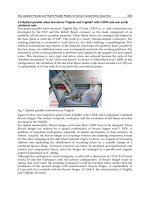
the manipulator base and platform respectively. With reference to Fig. 1, the platform pose
is described by the vector c = (O
p
– O
b
), which gives the origin of S
p
with respect to S
b
, and

by the proper orthogonal matrix R (i.e. det(R) = +1, R
T
R = 1 where 1 is the 3 × 3 identity
matrix) which describes the orientation of S
p
with respect to S
b
. In some applications, R is
defined equivalently as R = [r
1
r
2
r
3
]
T
, where the r
i
’s (i = 1,…, 3) are the 3 × 1 orthonormal
vectors (i.e. r
i
⋅ r
j
= 0 if i ≠ j and r
i
⋅ r
j
= 1 if i = j) indicating the components of the unit vectors
of the frame S
b

in the frame

S
p
. With reference to Fig. 2, consider the leg variables
ϕ
i1
,
ϕ
i2
and
l
i
which define the position of points P
i
with respect to S
b
(without losing in generality, in the
following it is assumed that the leg geometry is such that the leg unit vector v
i
,
v
i
= B
i
P
i
/|B
i
P

i
|, is orthogonal to the axis u
i
of the revolute pair R
i2
and that the unit vector u
i

is orthogonal to the axis i
i
of the revolute pair R
i1
; thus,
ϕ
i1
indicates the angle between axes
u
i
and j
i
,
ϕ
i2
indicates the angle between the vector P
i
B
i
and the axis i
i
, and l

i
indicates the
distance between points P
i
and B
i
). By definition, the DPA of 6-DOF UPS-PMs having n legs
consists in finding c and R once the magnitude of at least 6 leg variables (among the 3n
possible variables
ϕ
i1
,
ϕ
i1
and l
i
, for i = 1, …, n) are known by measurement. In practice, c
and R are found as the solution of a system of kinematic constraint equations (SKCE) of the
type

(
)
ϕϕ
12
,; , ,
iiii
l=R
f
c0, i = 1, …, n. (1)
For the class of manipulators under study, the kinematic constraint equations (1) can be

derived by considering the analytical expressions of vectors B
i
P
i
(i = 1, …, n). Indeed, by
referring to Fig. 1, the position vector q
i
= (P
i

−
B
i
)
b
expressed in S
b
can be written as

=
+−
iii
Rqc pb, (2)
where p
i
= (P
i

−
C)

p
and b
i
= (B
i

−
O)
b
are known (at the outset) position vectors expressed in
S
p
and S
b
respectively. Besides, with reference to Fig. 2, the position vector q
i
can also be
written as
q
iii
=lv , (3.1)
Robust, Fast and Accurate Solution of the Direct Position Analysis of
Parallel Manipulators by Using Extra-Sensors

145

ϕ
ϕ
+×
22

cos sin
ii i ii i
=vi ui , (3.2)

ϕ
ϕ
cos sin
ii i1 i i1
=uj k− , (3.3)
where, of course, in Eqs. (3) vectors i
i
, j
i
, k
i
, u
i
and v
i
are assumed to be expressed in S
b
.
Starting from Eqs. (2) and (3), different sets of rather simple linear kinematic constraint
equations (KCE) can be derived for each of the sensor layouts R
RP, RRP and RRP. Indeed, if
the i-th leg is equipped with one sensor according to the layout R
RP, then the angle
ϕ
i1
(and

the vector u
i
) are fully known. Therefore, from equations (2), (3.1) and (3.2) the following
KCE can be written:

(
)
+−=
T
iiii
uu Rcpb 0 , (4)
which indicates that the distance of the platform point P
i
from the plane passing through B
i

and having the measured vector u
i
as normal (i.e. the plane defined by i
i
and v
i
) is zero.
Note that Eq. (4) consists of three equations among which only one is independent of the
others. If the leg is equipped with two sensors according to the layout RR
P, then the angles
ϕ
i1
and
ϕ

i2
(and the vector v
i
) are fully known. Therefore, from equations (2) and (3.1) the
following KCE can be written:

(
)
()
−+−=
T
ii i i
1vv Rcpb 0, (5)
which indicates that the distance of the platform point P
i
from the line passing through B
i

and directed along the measured vector v
i
is zero. Note that Eq. (5) consists of three
equations among which only two are independent of the others. If the leg is equipped with
three sensors according to the layout RRP
, then the angles
ϕ
i1
and
ϕ
i2
, and the length l

i
(and
the vector q
i
) are fully known. Therefore, from equations (2) and (3.1) the following KCE can
be written:

(
)
+−−=
ii ii
lRvcpb 0, (6)
which indicates that the distance of the platform point P
i
from the corresponding measured
point lying on the leg is zero. Note that Eq. (6) consists of three independent equations.
Equations (4)-(6) are of the type described by Eq. (1). Considering all the instrumented legs
of the manipulator and by resorting to a unified formulation, the SKCE of Eq. (1) can be
written as

(
)
δ
+−− =
iiiii
WR vcpb 0, i =1, …, n (7)
where W
i
= u
i

u
i
T
and
δ
i
= 0, W
i
= 1 - v
i
v
i
T
and
δ
i
= 0, or W
i
= 1 and
δ
i
= l
i
if the i-th leg is
instrumented according to the sensor layout R
RP, RRP or RRP respectively. The SKCE of
Eq. (7) consists of 3n equations. If the manipulator is equipped with at least nine sensors,
then nine linearly independent equations can usually be extracted from Eq. (7) to find the
actual manipulator configuration. Indeed, such nine equations can be used to determine the
three components of c and six of the nine components of R (for instance the components of

the orthonormal vectors r
1
and r
2
); the remaining three components of R (the components of
the orthonormal vector r
3
) can be determined afterwards by using a further three linear
Parallel Manipulators, Towards New Applications

146
equations coming from the proper orthogonality conditions (the three equations r
1
⋅ r
3
= 0,
r
2
⋅ r
3
= 0 and det(R) = +1). Among all the possible sensor layouts, the sets {n-RRP} (n ≥ 3)
guarantee that a unique DPA solution can always be found. For other sensor layouts,
manipulator configurations may exist for which the set of measurement data is singular and,
thus, nine linearly independent equations cannot be extracted from Eq. (7).
4.2 The general method: general sensor layout with measurement errors
The equalities described by Eq. (7) hold in ideal situations only. Indeed, whenever finite
precision arithmetic is used to perform the required calculation and whenever joint-sensor
readouts are affected by measurement errors, the following relations

(

)
δ
+−− =
iiiii i
WR vcpb e
, i =1, …, n, (8)
hold instead of Eqs. (7), where the e
i
’s are error vectors whose magnitude should be as small
as possible. In such real situations, the DPA can be recast to the solution of the following
constrained least-squares (CLS) problem
()
[]
2
1
,
min
n
iiiii
i
δ
=
+−−
∑
R
WR v
c
cpb ,
subject to R
T

R = 1 and det(R) = +1.
(9)
By observing the quadratic nature of the function to be minimized, the solution of Eq. (9) is
reduced to first solving the following CLS problem in R only
2
1
11
min
nn
ii jjii
ij
−
==
′
′
−−−
⎡
⎤
⎡⎤
⎞
⎛
⎢
⎥
⎟
⎢⎜ ⎥
⎜⎟
⎢
⎥
⎢⎥
⎝

⎠
⎣⎦
⎣
⎦
∑∑
R
WR W WRppbv,
subject to R
T
R = 1 and det(R) = +1,
(10.1)
and then to computing c as

()
1
1
n
jj jj jj
j
δ
−
=
=− − −
⎡
⎤
⎣
⎦
∑
W
WR W vcpb

, (10.2)
where the 3 × 3 matrix W
, and the 3 × 1 vectors b′
i
and v′
i
are

1
n
j
j=
=
∑
W
W
, (10.3)

1
1
n
ii jj
j
−
=
′
−
=
∑
WWbb b

, (10.4)

1
1
n
iii jj
j
δ
δ
−
=
′
−
=
∑
W
vvv , (10.5)
Robust, Fast and Accurate Solution of the Direct Position Analysis of
Parallel Manipulators by Using Extra-Sensors

147
and depend on the given manipulator geometry and on the measured joint variables. In
general, the closed-form solution of the CLS problem described by Eq. (10.1) is difficult to
compute. In practice, an acceptable minimizer R of Eq. (10.1) can be obtained by evaluating
the orthogonal polar factor (OPF) of the solution of the corresponding unconstrained least-
square (ULS) problem, which is given in the following

−−
⎡⎤
⎢⎥

⎢⎥
⎢⎥
⎣⎦
bv
123
1
2
,,
3
min
WWW
rrr
r
Pr
r
, (11.1)

nn
′
=
′
⎡
⎤
⎢
⎥
⎢
⎥
⎢
⎥
⎣

⎦
11

W
W
W
b
b
b
, (11.2)

n
′
=
′
⎡
⎤
⎢
⎥
⎢
⎥
⎢
⎥
⎣
⎦
1

W
v
v

v
, (11.3)

1
1

j
j
−
=
−
=
−
=
−
⎡
⎤
⎞
⎛
⎟
⎢
⎜⎥
⎜⎟
⎢
⎥
⎝
⎠
⎢
⎥
⎢

⎥
⎢
⎥
⎞
⎛
⎢
⎥
⎟
⎜
⎢
⎥
⎜⎟
⎝
⎠
⎣
⎦
∑
∑
1
11
1
n
jj
n
nn jj

W
WP W WP
P
WP W WP

, (11.4)

=
⎡
⎤
⎢
⎥
⎢
⎥
⎢
⎥
⎢
⎥
⎣
⎦
p
00
0p0
00p
TTT
i
TTT
ii
TTT
i
P , (11.5)
where
P
W
is a 3n × 9 matrix, P

i
(i =1, …, n) is a 3 × 9 matrix, and b
W
and v
W
are 3n × 1 vectors.
Hence, an acceptable minimizer of Eq. (10.1) is

(
)
ˆ
OPF=RR, (12.1)

[]
ˆ
ˆˆˆ
123
=Rrrr
T
, (12.2)

()
()
ˆ
ˆ
ˆ
1
1
2
3

TT
−
=+
⎡⎤
⎢⎥
⎢⎥
⎢⎥
⎣⎦
WW W W W
r
rPPP
r
bv
, (12.3)
Parallel Manipulators, Towards New Applications

148
where the vectors
ˆ
1
r ,
ˆ
2
r and
ˆ
3
r are estimates of the orthonormal vectors r
1
, r
2

and r
3
.
Regarding the meaning of the orthogonal polar factor, note that given a 3
× 3 matrix A
whose polar decomposition is
A = QM, where Q is an orthogonal 3 × 3 matrix and M is a
symmetric and positive definite 3
× 3 matrix, then OPF(A) = Q. Providing that matrix
T
W
W
PP
is well conditioned (i.e. if rank(
P
W
) = 9), then Eqs. (12) admit a unique solution
corresponding to the actual orientation of the manipulator platform.
4.2.1 Uniqueness of the solution and computational issues
According to Eqs. (12), the actual platform orientation can be found if rank(P
W
) = 9. In order
for
P
W
to have full rank, a minimum of nine leg variables need to be measured. However,
this may not be sufficient. Indeed, due to matrices
W
i
and P

i
(i = 1, …, 6), matrix P
W
is
dependent on the given manipulator geometry and on the configuration (which is known by
measurements). As a matter of fact, special manipulator configurations may exist for which
rank(
P
W
) < 9. In practice, for given manipulator geometry and for selected sensor layout, a-
priori study of the rank of
P
W
is required in order to prevent the method to fail. In cases
where the drop of rank (which may be caused not only by special configurations and a
special manipulator geometry, but also by the availability of less than nine joint-sensor
measurements) is not too drastic, a number of remedies that rely on the mutual dependency
of the components of
R exist, which make it possible to find the actual manipulator
orientation. A first trick (trick 1) consists in circumventing the rank deficiency by solving
Eqs. (11) for a reduced number of unknowns only (whose number cannot be greater than the
rank of
P
W
) and by calculating the remaining ones via the proper orthogonality conditions.
As an example, note that the solution of Eqs. (11) for the components of
ˆ
1
r
and

ˆ
2
r
only, and
the a-posteriori evaluation of the components of
ˆ
3
r via the three linear equations
ˆˆ
13
0⋅=rr ,
ˆˆ
23
0⋅=rr and
ˆ
det( )
R = +1, requires rank(P
W
) ≥ 6 only. A second trick (trick 2) consists in
restoring the rank of
P
W
by considering, in addition to the points P
i
(i = 1, …, n) of the
instrumented legs, additional virtual points
P
k
(k > n) depending on the P
i

’s themselves such
that
p
k
= p
i
× p
j
and (b′
k
+ v′
k
) = (b′
i
+ v′
i
) × (b′
j
+ v′
j
), (i ≠ j; for i,j = 1, …, n). As an example
note that whenever the third components of the vectors
p
i
’s are zero for all points P
i
(i = 1,
…,
n), then rank(P
W

) ≤ 6. In this case, the rank of P
W
can be restored to 9 by adding an
appropriate number of virtual points as defined above. A third last trick (trick 3) consists in
circumventing the rank drop of
P
W
by solving the rank deficient least-squares problem
given by Eqs. (11) via a method based on the singular value decomposition (SVD) of
P
W

(Golub & Van Loan, 1983). Among the three remedies, trick (3) is the most general (it does
not require a-priori knowledge of the structure of
P
W
), rather accurate, but it is also the most
computationally intensive; trick (2) is quite general (it requires some a-priori knowledge of
the structure of
P
W
) and quite computationally efficient, but it is the most inaccurate; trick
(1) is the less general (it requires a-priori knowledge of the full structure of
P
W
), it is quite
accurate and quite computationally efficient.
4.3 A novel method for the manipulator actual configuration determination
As described in sub-section 4.2.1, the effectiveness of the general method relies upon the
good conditioning of

P
W
. A very practical sensor layout which both guarantees that the rank
of
P
W
is independent of manipulator configuration and greatly simplifies the solution of the
DPA is the set {
n-RRP} (n ≥ 3). With this sensor layout, the DPA problem described by
Eqs. (10) is reduced to
Robust, Fast and Accurate Solution of the Direct Position Analysis of
Parallel Manipulators by Using Extra-Sensors

149
F
min −−
R
RP B V ,
subject to
R
T
R = 1 and det(R) = +1,
(13.1)
and

=
+−Rcbv p, (13.2)
where
p, b and v are the following 3 × 1 mean vectors

1
1
n
j
j
n
=
=
∑
p
p
, (13.3)

1
1
n
j
j
n
=
=
∑
bb
, (13.4)

1
1
n
jj
j

l
n
=
=
∑
vv
, (13.5)
and
P, B and V are the following 3 × n matrices

[
]

1 n
′
′
=P
p
p , (13.6)

[
]

1 n
′
′
=B
bb, (13.7)

[

]

1 n
′
′
=V
vv, (13.8)
which are formed, respectively, by the 3
× 1 vectors p′
i
= (p
i
– p), b′
i
= (b
i
– b) and
v′
i
= (v
i
– v). It is worth highlighting that the quantities p, b, P and B depend only on the
manipulator geometry, while
v and V depend also on the manipulator configuration. As
usual, the notation ║
A║
F
appearing in Eq. (13.1) is used to indicate the Frobenius norm of
matrix
A. Equations (13) show that if the center O

p
of the mobile frame S
p
is chosen as the
centroid of points
P
i
(i = 1, …, n), i.e. p = 0, then the orientation and the position problems
are decoupled, i.e.
c = (b + v).
Following the procedure based on the ULS estimate which was described in section 4.2, an
acceptable minimizer
R of the CLS problem described by Eq. (13.1) is

(
)
ˆ
OPF
=RR
, (14.1)

()
(
)
ˆ
1
TT
−
=+RBVPPP . (14.2)

However, for the set {n-RRP} (n ≥ 3), the optimal solution of Eq. (13.1) can be found in
closed-form. Indeed, the CLS problem described in Eq. (13.1) is well known in computer
vision (Umeyama, 1991) and admits the following solution
Parallel Manipulators, Towards New Applications

150

(
)
(
)
=
⎡
⎤
⎣
⎦
diag 1,1,det
T
RU US S, (15.1)
where
U and V are the 3 × 3 matrices coming from the SVD of the cross-covariance matrix

()
T
=+CBVP. (15.2)
That is,
C = UDS
T
(UU
T

= SS
T
= 1 and D = diag(d
1
, d
2
, d
3
), d
1
≥ d
2
≥ d
3
≥ 0). The unique
solution given by Eq. (15) does not require the full rank of
C (Umeyama, 1991). As a matter
of fact, the actual platform orientation can be computed whenever rank (
C) ≥ 2.
The solution given in Eq. (15) is different from that proposed in (Baron and Angeles, 2000)

(
)
OPF=RC, (16)
which is the solution of the orthogonal Procrustes problem (Golub & Van Loan, 1983)
obtained from the CLS problem of Eq. (13.1) by relaxing the constraint det(
R) = +1.
4.4 Comparison of different DPA methods in terms of accuracy and computational
efficiency
Among the different solution methods represented by equations (14), (15) and (16), only

Eqs. (15) always provides the exact minimum of the CLS problem given by Eq. (13). Thus,
only the solution given by Eqs. (15) always corresponds to the actual platform orientation
and is the most accurate. Indeed, the solutions given by Eqs. (14) and Eq. (16) do not
guarantee the proper orthogonality (det(
R) = +1) of matrix R. This is rather risky since
Eqs. (14) and Eq. (16) may fail to give the correct rotation matrix (corresponding to the
actual manipulator configuration) and may give a reflection instead when the sensor
readouts are affected by measurement errors (this drawback is more severe the larger the
measurement errors are). Between the solutions given by Eqs. (14) and Eq. (16), the former is
the least accurate. Indeed, Eqs. (14) do not even minimize Eq. (13.1) (Eqs. (14) can be a viable
good estimate of the solution in cases where measurement errors are rather small only).
Moreover, due to the matrix inversion operation, note that Eqs. (14.2) requires matrix
P to
have full rank. This is not the case whenever points
P
i
’s (i = 1, …, n) are coplanar. In such
instances, as already described in section 4.2.1, to obtain the solution of Eq. (14.2) it is
necessary to resort to either trick (2), which however leads to a rather inaccurate solution, or
trick (3), which however implies a large computational effort.
In terms of computational efficiency, it is worth highlighting that the solution represented
by Eqs. (15) requires the calculation of the SVD of a 3
× 3 matrix, while the solutions
represented by equations (14) and (16) require the calculation of the polar decomposition
(PD) of a 3
× 3 matrix. In general the algorithms available for the computation of the PD are
more efficient than those available for the computation of the SVD. However, when 3
× 3
matrices are of concern, fast and robust solutions of the SVD exist which require fewer
calculations than those required by the PD of 3

× 3 matrices. As a matter of fact, the SVD of a
3
× 3 matrix can be obtained via non-iterative algorithms. As an example, an improved
version of the algorithm presented in (Vertechy & Parenti-Castelli, 2004), which is based on
the analytical solution of the cubic equation, requires only 150 multiplications/divisions, 88
sums/subtractions, 5 square root evaluations and 4 trigonometric evaluations to obtain the
full SVD. Conversely, the algorithms available for the PD are iterative. In particular,
considering the most well known and adopted algorithms, the PD of 3
× 3 matrices via the
routine proposed in (Dubrulle, 1999) requires (87 +
k
D
⋅78) multiplications/divisions,
Robust, Fast and Accurate Solution of the Direct Position Analysis of
Parallel Manipulators by Using Extra-Sensors

151
(47 + k
D
⋅39) sums/subtractions and (4 + k
D
⋅3) square root evaluations, where k
D
is the
number of iterations required by the Dubrulle’s routine to converge; and the PD of 3 × 3
matrices via the routine proposed in (Higham, 1986) requires (48 +
k
H
⋅63)
multiplications/divisions, (38 +

k
H
⋅62) sums/subtractions and (k
H
⋅3) square root evaluations,
where
k
H
is the number of iterations required by Higham’s routine to converge. In practice,
simulations of the DPA solution of UPS-PMs employing both Dubrulle’s and Higham’s
routines show that
k
D
> 3 and k
H
> 2 when solving Eq. (14.1), and that k
D
> 5 and k
H
> 5
when solving Eq. (16). Note that the solution of Eq. (16) requires more iterations than those
of Eq. (14.1) since matrix
ˆ
R
is closer to orthogonality than matrix C.
Finally, it is worth mentioning that both Dubrulle’s and Higham’s routines involve the
matrix inversion operation of either
ˆ
R
or C and, thus, both Eq. (14.1) and Eq. (16) require

such matrices to have full rank. Again, this is not the case whenever points
P
i
‘s (i = 1, …, n)
are coplanar, and this requires resorting to either trick (2), which leads to a rather inaccurate
solution, or trick (3). In this latter case, once the SVD of either
C or
ˆ
R is calculated (i.e.
either
C = UDV
T
or
ˆ
T
=RUDV), the solution of Eq. (14.1) and Eq. (16) is found as R = UV
T
.
Hence, generally, in order to find a unique and accurate solution of the DPA, the
computation of the SVD of either
C or
ˆ
R
is anyway required.
5. Conclusions
This chapter addresses the solution of the direct position analysis (DPA) of parallel
manipulators. More specifically, it focuses on the determination of the actual configuration
of parallel manipulators, which have legs of type UPS (where U, S and P are for universal,
spherical and prismatic pairs respectively), by using extra-sensor data, that is a number of
sensor data which is greater than the number of manipulator degrees of freedom. First, an

extensive overview of the extra-sensor approaches that are available in the literature for the
solution of the manipulator direct position analysis is provided. Second, a general method is
described which makes it possible to solve accurately and in real-time the DPA of
manipulators having general architecture, general sensor layouts and sensor data affected
by measurement errors. The method, however, may suffer from singularities of the set of
sensor data. Third, a novel method is presented which, by exploiting a suitable sensor
layout, makes it possible to solve robustly, accurately and in real-time the direct position
analysis of manipulators having general architecture and sensor data affected by
measurement errors. A comparison with other methods based on mathematical proofs is
provided that shows the accuracy and the computational efficiency of the proposed novel
method.
6. References
Angeles, J. (1990). Rigid-body pose and twist estimation in the presence of noisy redundant
measurements,
Proc. Eighth CISM-IFToMM Symposium on Theory and Practice of
Robots and Manipulators, pp. 69-78, Cracow, July 2-6 1990
Baron, L. & Angeles, J. (1994). The measurement subspaces of parallel manipulators under
sensor redundancy,
ASME Design Automation Conf., pp. 467-474, Minneapolis, 11-14
September 1994
Baron, L. & Angeles, J. (1995). The isotropic decoupling of the direct kinematic of parallel
manipulators under sensor redundancy,
IEEE Int. Conf. on Robotics and Automation,
pp. 1541-1546, Nagoya, 25-27 May 1995
Parallel Manipulators, Towards New Applications

152
Baron, L. & Angeles, J. (2000a). The direct kinematics of parallel manipulators under joint-
sensor redundancy.
IEEE Trans. on Robotics and Automation, Vol. 16, No. 1, 12-19

Baron, L. & Angeles, J. (2000b). The kinematic decoupling of parallel manipulators using
joint-sensor data.
IEEE Trans. on Robotics and Automation, Vol. 16, No. 6, 644-651
Bonev, I.A. & Ryu J. (2000). A new method for solving the direct kinematics of general 6-6
Stewart platforms using three linear extra sensors.
Mechanism and Machine Theory,
Vol. 35, No. 3, 423-436
Bonev, I.A.; Ryu, J.; Kim, S G. & Lee, S K. (2001). A closed-form solution to the direct
kinematics of nearly general parallel manipulators with optimally located three
linear extra sensors.
IEEE Transactions on Robotics and Automation, Vol. 17, No. 2,
148-156
Cappel, K.L (1967). Motion simulator.
US Patent #3295224
Charles, P.A S. (1995). Octahedral machine tool frame.
US Patent #5392663
Cheok, K.C.; Overholt, J.L. & Beck, R.R. (1993). Exact Method for Determining the
Kinematics of a Stewart Platform Using Additional Displacement Sensors.
Journal of
Robotic Systems
, Vol. 10, No. 5, 689-707
Chiu, Y.J. & Perng, M H. (2001). Forward kinematics of a general fully parallel manipulator
with auxiliary sensors.
Int. J. of Robotics Research, Vol. 20, No. 5, 401-414
Daniel, R.W.; Fischer, P.J. & Hunter, B. (1993). A High Performance Parallel Input Device.
Proc. SPIE Vol. 2057, Telemanipulator Technology and Space Telerobotics, pp. 272-281,
Boston, December 1993
Di Gregorio, R. & Parenti-Castelli, V. (2002). Fixation devices for long bone fracture
reduction: an overview and new suggestions.
Journal of

Intelligent and Robotic Systems, Vol. 34, No. 3, 265-278
Dubrulle, A.A. (1999). An optimum Iteration for the Matrix Polar Decomposition.
Electronic
Transactions on Numerical Analysis, Vol. 8, 21-25
Etemadi-Zanganeh, K. & Angeles, J. (1995). Real time direct kinematics of general
six-degree-of-freedom parallel manipulators with minimum sensor data.
Journal of
Robotics Systems, Vol. 12, No. 12, 833-844
Faugere, J.C. & Lazard, D. (1995). The combinatorial classes of parallel manipulators.
Mechanism and Machine Theory, Vol. 30, No. 6, 765-776
Fenton, R.G. & Shi, X. (1989). Comparison of methods for determining screw parameters of
finite rigid body motions from initial positions and final position data, in
Advances
in Design Automation, Vol. 3, 433-439
Gaillet, A. & Reboulet, C. (1983). An Isostatic Six Component Force and Torque Sensor.
Proc. 13th Int. Symposium on Industrial Robotics, pp. 102-111, Chicago, 18-21 April
1983
Geng, Z. & Haynes, L.S. (1994). A 3-2-1 kinematic configuration of a Stewart platform and
its application to six degree of freedom pose measurements.
Robotics & Computer-
Integrated Manufacturing
, Vol. 11, No. 1, 23-34
Golub, G.H. & Van Loan, C.F. (1983).
Matrix Computations, The Johns Hopkins University
Press, ISBN 0-946536-00-7, Baltimore
Gough, V.E. & Whitehall, S.G. (1962). Universal Tire Test Machine.
Proceedings 9
th
Int.
Technical Congress F.I.S.I.T.A

, Vol. 117, pp. 117-135, London, 30 April – 5 May 1962
Griffis, M. & Duffy, J. (1989). A Forward Displacement Analysis of a Class of Stewart
Platform.
Journal of Robotics Systems, Vol. 6, No. 6, 703-720
Han, H.; Chung, W. & Youm, Y. (1996). New Resolution Scheme of the Forward Kinematics
of Parallel Manipulators Using Extra Sensors.
ASME Journal of Mechanical Design,
Vol. 118, No. 2, 214-219
Hesselbach, J.; Bier, C.; Pietsch, I.; Plitea, N.; Büttgenbach, S.; Wogersien, A. & Güttler, J.
(2005). Passive-joint sensors for parallel robots.
Mechatronics, Vol. 15, 43-65
Robust, Fast and Accurate Solution of the Direct Position Analysis of
Parallel Manipulators by Using Extra-Sensors

153
Higham, N.J. (1986). Computing the Polar Decomposition – with Applications. SIAM Sci.
Stat. Comput.
, Vol. 7, No. 4, 1160-1174
Innocenti, C. & Parenti-Castelli, V. (1990). Direct Position Analysis of the Stewart Platform
Mechanism.
Mechanism and Machine Theory, Vol. 25, No. 6, 611-621
Innocenti, C. & Parenti-Castelli, V. (1991). A Novel Numerical Approach to the Closure of
the 6-6 Stewart Platform Mechanism.
ICAR’91, Fifth Int. Conf. on Advance Robotics,
pp. 851-855, Pisa, 19-22 June
Innocenti, C. & Parenti-Castelli, V. (1993). Echelon Form Solution of Direct Kinematics for
the General Fully-Parallel Spherical Wrist.
Mechanism and Machine Theory, Vol. 28,
No. 4, 553–561.
Innocenti, C. & Parenti-Castelli, V. (1994). Exhaustive Enumeration of Fully Parallel

Kinematic Chains,
ASME International Winter Annual Meeting DSC-55-2,
pp. 1135-1141, Chicago, November 1994.
Innocenti, C. (1998). Closed-Form Determination of the Location of a Rigid Body by Seven
In-Parallel Linear Transducers.
ASME Journal of Mechanical Design, Vol. 120, 293-298
Innocenti, C. (2001). Forward Kinematics in Polynomial Form of the General Stewart
Platform.
ASME Journal of Mechanical Design, Vol. 123, 254-260
Jacobsen, S.C. (1975). Rotary-to-Linear and Linear-to-Rotary Motion Converters.
US Patent
#3864983
Jin Y. (1994). Exact solution for the forward kinematics of the general stewart platform using
two additional displacement sensors.
Proc. of the 23
rd
ASME Mechanism Conference,
DE-Vol. 72, pp. 491-495, Minneapolis, 11-14 September 1994
Jin, Y. & Hai-rong, F. (1996). Explicit Solution for the Forward Displacement Analysis of the
Stewart Platform Manipulator.
Proc. ASME DETC 1996, Irvine, 18-22 August 1996
Lee, T Y. & Shim, J K. (2001). Forward kinematics of the general 6-6 Stewart platform
using algebraic elimination.
Mechanism and Machine Theory, Vol. 36, No. 9,
1073-1085
Lewis, J.L.; Carroll, M.B.; Morales, R.H. & Le, T.D. (2002). Androgynous, reconfigurable
closed loop feedback controlled low impact docking system with load sensing
electromagnetic capture ring.
US Patent #6354540
McAree, P.R. & Daniel, R.W. (1996). A Fast, Robust Solution to the Stewart Platform

Forward Kinematics.
Journal of Robotics Systems, Vol. 13, No. 7, 407-427
McCallion, H. & Truong, P.D. (1979). The Analysis of a Six-Degree-of-Freedom Work Station
for Mechanised Assembly.
Proceedings of the Fifth World Congress on Theory of
Machines and Mechanisms, 611-617, Montreal, July 1979.
Merlet, J-P. (1992). Direct Kinematics and Assembly Modes of Parallel Manipulators.
The
International Journal of Robotics Research, Vol. 11, No. 2, 150-162
Merlet, J-P. (1993a). Direct Kinematics of Parallel Manipulators.
IEEE Transactions on Robotics
and Automation, Vol. 9, No. 6, 842-845
Merlet, J-P. (1993b). Closed-Form Resolution of the Direct Kinematics of Parallel
Manipulators Using Extra Sensors Data.
Proc. IEEE Int. Robotics and Automation
Conf., pp. 200-204, Atlanta, 2-7 May 1993.
Nair, R. & Maddocks, J.H. (1994). On the Forward Kinematics of Parallel Manipulators.
The
Int. Journal of Robotics Research
, Vol. 13, No. 2, 171-188
Nanua, P.; Waldron, K.J. & Murty, V. (1990). Direct Solution of a Stewart Platform.
IEEE
Transaction on Robotics and Automation, Vol. 6, No. 4, 438-443
Nguyen, C.C.; Antrazi, S.S. & Zhou, Z.L. (1991). Analysis and Implementation of a 6 DOF
Stewart Platform-Based Force Sensor for Passive Compliant Robotic Assembly.
IEEE Proc. of the Southeast Conf'91, pp. 880-884, Williamsburg, 7-10 April 1991
Parenti-Castelli, V. & Di Gregorio, R. (1995). A Three Equations Numerical Method for the
Direct Kinematics of the Generalized Gough-Stewart Platform.
9th World Congress
Parallel Manipulators, Towards New Applications

154
on the Theory of Machines and Mechanisms
, pp. 837-841, Milan, 30 August – 2
September 1995.
Parenti-Castelli, V. & Di Gregorio, R. (1998). Real-Time Computation of the Actual Posture
of the General Geometry 6-6 Fully-Parallel Mechanism using Two Extra Rotary
Sensors.
Journal of Mechanical Design, Vol. 120, No. 4, 549-554
Parenti-Castelli, V. & Di Gregorio, R. (1999). Determination of the Actual Configuration of
the General Stewart Platform Using Only One Additional Sensor.
Journal of
Mechanical Design, Vol. 121, No. 1. 21-25
Parenti-Castelli, V. & Di Gregorio, R. (2000). A new algorithm based on two extra sensors for
real-time computation of the actual configuration of the generalized Stewart-Gough
manipulator.
ASME J. of Mechanical Design, Vol. 122, No. 3, 294-298
Reboulet, C. (1988). Robot parallèles.
Technique de la Robotique, Hermes (Ed.), Paris
Schmidt-Kaler, T. (1992). The Hexapod Telescope: A New Way to Very Large Telescopes.
Progress in Telescope and Instrumentation Technologies, ESO Conference and Workshop
Proceedings, ESO Conference on Progress in Telescope and Instrumentation Technologies
,
p. 117, European Southern Observatory (ESO), Garching, 27-30 April 1992.
Shi, X. & Fenton, R.G. (1991). Forward Kinematic Solution of a General 6 DOF Stewart
Platform Based on Three Point Position Data.
Eight World Cong. on the Theory of
Machines and Mechanism
, 1015-1018, Prague, 26-31 August 1991.
Stewart, D. (1965). A Platform with Six Degree of Freedom.

Proc. of the Institution of
Mechanical Engineers, vol. 180, No. 15, 371-386
Stoughton, R. & Arai, T. (1991). Optimal sensor placement for forward kinematics
evaluation of a 6-dof parallel link manipulator.
IEEE Int. Conf. on Intelligent Robots
and Systems, IROS’91, pp. 785-790, Osaka, 3-5 November 1991.
Taylor, H.S. & Taylor, J.C. (2000). Six axis external fixator strut.
US Patent#6030386
Tancredi, L. & Merlet, J P. (1994). Evaluation of the errors when solving the direct
kinematics of parallel manipulators with extra sensors, In: Advances in Robot
Kinematics and Computational Geometry, Lenarcic J. and Ravani B., (Ed), 439-448,
Springer, ISBN:978-0-7923-2983-1
Tancredi, L.; Teillaud, M. & Merlet, J P. (1995). Extra sensors data for solving the forward
kinematics problem of parallel manipulators.
9th IFToMM World Congress on the
Theory of Machines and Mechanisms, pp. 2122-2126, Milan, 30 August-2 September
1995
Umeyama, S. (1991). Least-Squares Estimation of Transformation Parameters Between Two
point Patterns.
IEEE Transactions on Pattern Analysis and Machine Intelligence, Vol. 13,
No. 4, 376-380
Vertechy, R.; Dunlop, G.R. & Parenti-Castelli ,V. (2002). An accurate algorithm for the real-
time solution of the direct kinematics of 6-3 Stewart platform manipulators, In:
Advances in Robot Kinematics: Theory and Applications, Lenarcic J. & Thomas F., (Ed.),
369-378, Springer, ISBN: 978-1-4020-0696-8
Vertechy, R. & Parenti-Castelli, V. (2004). A fast and Accurate Method for the Singular Value
Decomposition of 3x3 Matrices, In:
On Advances in Robot Kinematics, Lenarcic J. and
Galletti C., (Ed.), 3-12, Springer, ISBN: 978-1-4020-2248-7
Vertechy, R. & Parenti-Castelli, V. (2006). Synthesis of 2-DOF Spherical US Parallel

Mechanisms, In:
Advances in Robots Kinematics: Mechanisms and Motion, Lenarcic J.
and Roth B., (Ed.), 385-394, Springer, ISBN: 978-1-4020-4940-8
Vertechy, R. & Parenti-Castelli, V. (2007). Accurate and Fast Body Pose Estimation by Three
Point Position Data.
Mechanism and Machine Theory, Vol. 42, No. 9, 1170-1183

8
Kinematic Modeling, Linearization
and First-Order Error Analysis
Andreas Pott† and Manfred Hiller‡
† Fraunhofer Institute for Manufacturing Engineering and Automation, Stuttgart
‡ Chair of Mechatronics, University of Duisburg-Essen,
Germany
1. Introduction
The kinematic analysis of parallel kinematic machines (PKM) is a challenging field, since
PKM are complex multi-body systems involving a couple of closed kinematic loops. It is
well-known that the forward kinematic function has in general no closed-form solution, and
that up to 40 different real solutions may exist for general geometry (Husty, 1996; Dietmaier,
1998). Therefore, an efficient and handy method is needed in practise, e.g. for design,
simulation, control, and calibration.
The analysis of manufacturing and assembly errors of manipulators is a topic that is highly
relevant for practical applications because the magnitude of these errors is directly coupled
to the total cost of production of the manipulator. In this setting, there exist intensive studies
on how to estimate the error of certain moving points, e.g. the tool center point, in terms of
the errors in the components of the mechanism (Brisan et al., 2002; Jelenkovic & Budin, 2002;
Kim & Choi, 2000; Song et al., 1999; Zhao et al., 2002), as well as how to allocate cost-optimal
tolerances to a mechanism (Chase et al., 1990; Ji et al., 2000). In this paper, an approach to
estimate the first-order influence of geometric errors on target quantities is suggested in
which linearization is performed by considering the force transmission of the manipulator.

This enables one to obtain a comprehensive model of linearized geometric sensitivities at a
low computational cost.
Error analysis for serial manipulators is relatively easy because one can establish an
analytical expression for the forward kinematics which maps the generalized joint and link
coordinates to the spatial displacements of the end-effector. There are numerous methods to
parameterize the forward kinematics, where the approach of Denavit and Hartenberg (1955)
is the most popular one. Once one has a closed-form expression for the forward kinematics,
one can take derivatives of it (with respect to the geometric parameters one is interested in)
and use these as sensitivity coefficients. In general, one introduces the sensitivity parameters
in such a way that they vanish at the nominal configuration. This is always possible by
introducing corresponding constant offsets where necessary.
For example, consider a robot involving a universal joint, and assume that the sensitivity to
errors in the fulfilment of the intersection property of the axes is to be analyzed. This can be
done by adding a parameter for the normal distance between the joint axes which is zero in
the nominal design, and with respect to which the partial derivative will yield the sought
sensitivity. However, such a method for sensitivity analysis results in a model with a
Parallel Manipulators, Towards New Applications

156
significant overhead. Examples of such models for joints are presented (Brisan et al., 2002;
Song et al., 1999). Some force-based methods for clearance analysis were introduced, which
are similar to the approach in this paper (Innocenti, 1999; Innocenti, 2002; Parenti-Castelli &
Venanzi, 2002 ; Parenti-Castelli & Venanzi, 2005).
A linearization method for complex mechanisms using the kinetostatic dualism and the
concept of kinematical differentials to efficiently set up the equations of motion of multi-body
systems has been proposed (Kecskeméthy & Hiller, 1994). Using this method, all required
partial derivatives can be described solely by using the kinematic transmission functions for
position and velocity, as well as the force transmission function of the system. Based on
these transmission functions, an algorithm is formulated for generating the Jacobian matrix
and the equations of motion through multiple evaluations of the kinematic transmission

functions for certain pseudo input velocities and accelerations. The corresponding
algorithms are denoted as kinematical differentials for the case of the pure kinematic
transmission function (Hiller & Kecskeméthy, 1989) and kinetostatic approach for the case of
use of force transmission (Kecskeméthy, 1994). Later, Lenord et al. (2003) showed that
kinematical differentials may be applied also to more general interdisciplinary systems
which also involve hydraulic components by using an exact linearization through the
kinematical differentials for the determination of the velocity linearization and numerical
differentiation for the calculation of the stiffness matrix of the hybrid system. Other authors
studied the determination of the stiffness matrix for complex multi-body systems using
explicit symbolic derivatives (El-Khasawneh & Ferreira, 1998; Rebeck & Zhang, 1999), taking
into account the stiffness of the actuators and the stiffness of special components. These
approaches however require numerous computational steps when many sensitivity
parameters are involved.
2. Kinematic modeling of parallel kinematic machines
2.1 Kinematic delimitation and geometry
In order to study a wide range of machine types, a generic approach for the modeling of
PKM is proposed (Pott, 2007). Since PKMs tend to be symmetric and different types of PKM
have similar components a modular design is used. In a first step the machine is divided
into three types of components: frames, platforms and legs (Fig. 1), which form the modules
of the kinetostatic code.

Fig. 1. Platform, legs, and machine frame modules of a generic six-degree-of-freedom
parallel kinematic machine
Kinematic Modeling, Linearization and First-Order Error Analysis

157
The machine frame defines the position and orientation of six pivot points A
i
. The mobile
platform introduces the position of six pivot point B

i
. Furthermore, the platform defines the
parameterization of the six-degrees-of-freedom (dof) of spatial motion at the tool center
point (TCP). Finally, different types of legs are introduced which mainly determine the
kinematic behaviour. The most common legs for PKMs are PUS, UPS and RUS structures
each consisting of an actuated prismatic (P) or revolute (R) joint as well as a pair of a
universal (U) and a spherical (S) joints. Each of these structures can be described by one
scalar constraint, as it is shown hereafter.


Fig. 2. Generic model of a spatial six-degree-of-freedom parallel kinematic machine
Each legs considered in this paper possess a pair of joints formed by a universal joint and a
spherical joint. For the analysis of the closed-kinematic chains, these joints are known as
characteristic pair of joints (Woernle, 1988). One can remove both of these joints and replace
this partial chain by one nonlinear scalar constraint. This constraint describes the
geometrical distance between the center of the universal joint and the center of the spherical
joint for the i-th leg as
a
i
+ l
i
= r + Rb
i
, (1)
where a
i
denotes the position vector of the pivot point on the base and b
i
is the relative
position of the pivot point with respect to the coordinate system fixed to the platform. The

Cartesian position and orientation of the platform frame K
TCP
is given by the vector r and
the orthogonal matrix R, respectively. The vector l
i
denotes the length of the leg. Solving
Eq. (1) for the magnitude l
i
² of the vector l
i
yields the system of six nonlinear constraints
(a
i
- r - Rb
i
)² - l
i
= 0 i=1,…,6. (2)
The world coordinates y consist of a parameterization of the position r and the orientation
matrix R. The geometry of the machine is expressed by the vectors a
i
, b
i
and l
i.
In the
following sections the definition of these vectors is introduced depending on the generalized
coordinate q
i
of the six actuators and the kinematic structure of the basic types of legs for

parallel kinematic machines.
The UPS legs are used in the Stewart-Gough-platforms which are often applied for motion
simulators of cars and aircrafts. The prismatic joint is actuated as linear actuator, e.g. by a
Parallel Manipulators, Towards New Applications

158
linear direct drive, ball bearing screw, hydraulic/pneumatic cylinder. For these mechanisms
the pivot points A
i
on the base
a
i
= c
i
(3)
are determined by the machine frame and fixed to a given position c
i
. The length of the strut
can be controlled by the drive through
l
i
= q
i +
q
o
(4)
where q
o
is a constant offset.
The PUS leg results from changing the order of the joints within the UPS leg. The universal-

spherical pair encloses a leg of constant length while the proximal pivot point is actuated
along a line. PUS legs are the basic leg components for Hexaglide, Linaglide and Linapod
PKM. They are described by the position vector c
i
and the direction u
i
. Thus, the position of
the proximal pivot point A
i
is defined as
a
i
= c
i
+ q
i
u
i
, (5)
where q
i
is the generalized coordinate of the drive. The length l
i
=const of the strut is given
by design.
Finally, the kinematics of the RUS leg is considered which is the basis of the Delta-robot
(Clavel, 1988). In contrast to the PUS leg, the proximal pivot points A
i
of RUS legs move a
circle defined by its center c

i
, an axis of rotation u
i
, and a lever v
i
which is given in its initial
position. Thus, it holds for the point A
i

a
i
= c
i
+ T(u
i,
q
i
) v
i
(6)
where T(u
,
q) is the rotation matrix for the axis u

and the angle q as it can be calculated by
Rodrigues formula. Again, for RUS legs the length of the strut l
i
=const is given by design.

Fig. 3. Geometric parameters of the leg-types under consideration
Kinematic Modeling, Linearization and First-Order Error Analysis

159
2.2 Review of the kinetostatic method
In the sequel, a short introduction to the kinetostatic method (Kecskeméthy, 1993;
Kecskeméthy, 1994) is given as a basis for the herewith presented linearization procedure.
Below, the basic equations of the kinetostatic transmission element are reviewed for better
reference in this paper. Details can be found in the cited papers. In the kinetostatic
formalism, mechanical components are modeled as transmission elements (Fig. 4) that map
the kinematic state q ,
q

, q

at the input to the kinematic state 'q , 'q

, 'q

at the output and
the associated generalized forces Q’ at the output to generalized forces Q at the input. The
kinetostatic state is composed of position, velocity, acceleration, and force. A mechanism is
divided into joints and links which transmit the state from one set of coordinate frames K
i

and scalar variables β
i
to another set {K
i
',β

i
'}. This concept allows one to model serial
manipulators as chains of transmission elements.


Fig. 4. General kinetostatic transmission element
Interestingly, the motion of closed kinematic loops can also be represented with the help of
transmission functions. For simple kinematic loops with one dof, this may be done in an
explicit form. In general, however, one has to employ iterative methods to solve the loops.
Nevertheless, in both cases one is able to compute the transmission function for position,
velocity, acceleration, and force.
Assuming that the position transmission function is given as y=φ(q), where q=[q
1
, …, q
n
]
T
is
a set of independent joint variables of the mechanism, the velocity transmission takes the
form

q
()
J( )
∂
==
ϕ
φ q
yqqq
q



(7)
For a given set of joint coordinates q, the twist y

of the end-effector frame (EEF) is a linear
combination of the joint rates
q

with the columns of the Jacobian J
q
acting as coefficient
vectors. Assuming ideal transmission behaviour within the transmission element, power is
neither generated nor consumed. Thus, virtual work at the input and the output can be set
equal, and one obtains

TT
''δ=δqQ q Q (8)
where the virtual displacements fulfil
q
'
δ
=δqJq. This yields
TTT
q
'δ=δqQ qJQ
and since this
holds for any
δq , the force transmission takes the form

T
q
'=QJQ. (9)
Parallel Manipulators, Towards New Applications

160
The relations (7) and (9) for velocity transmission and force transmission is called kinetostatic
duality. The basic idea of the kinematical differentials is to evaluate the velocity transmission
function
φ

for pseudo unit velocities
T
i
ˆ
q [0, ,1, ,0]=

with zeros everywhere up to the i-th
component in order to identify the i-th column of the Jacobian J
q
. Thus, the Jacobian J
q
can
be determined with n passes of velocity transmission. This method is called velocity-based
Jacobian algorithm. By exploiting kinetostatic duality, this algorithm can be analogously
applied to force transmission yielding the force-based Jacobian algorithm. Here the Jacobian
J
q

is computed row-wise by setting unit pseudo forces

T
i
ˆ
[0, ,1, ,0]=Q
with zeros
everywhere besides the i-th component, performing the force mapping (9), and storing the
resulting vector of generalized forces
i
ˆ
Q
at the input as the i-th row of J
q
. Thus, the Jacobian
can be computed row-wise by six force transmissions for a general manipulator
independently of the number of input parameters. This Jacobian evaluation procedure shall
be further exploited here.
The complete kinetostatic formalism is implemented in the object-oriented programming
library Mobile that uses the C++ programming language (Kecskeméthy, 1994), and a
differential geometric interpretation of the kinetostatics has been given in (Kecskeméthy,
1993).
2.3 Modular modeling of parallel kinematic machines
As already mentioned before, the PKM is subdivided into the modules platform, frame, and
legs. These components are the foundation of a modular kinetostatic model, which
automatically assembles and solves the system of nonlinear constraints. The expressions
introduced for the different legs in section 2.1 can be used to calculate the relative
kinematics of the different types of PKM. By means of the kinetostatic method, C++ classes
for the elementary components of multi-body systems, i.e. prismatic joints, revolute joints,
and rigid bodies as well as the constraint solvers for kinematic loops are used for the
modeling. These elements defined the required transmission functions for position, velocity,
acceleration, and force. Thus, if the machine can be automatically assembled from these

classes, one receives a comprehensive tool for the kinematic analysis of parallel robots.
A class called generic machine assembles a kinetostatic model from the components
introduced above. Firstly, the legs is attached to the platform and to the frame. For the
forward kinematics the legs provide constraints that characterize which motions can be
transmitted. The generic machine assembly module collects the constraints from the legs
and the generalized coordinates from the platform in order to combine them to a nonlinear
system of equations. Then a numerical procedure like a Newton-Raphson-algorithm is
applied to solve the forward kinematics. Once the position of the platform is determined
one can use local methods from the legs to calculate the complementary variables of the
passive joints in each kinematic loop.
The module frame defines the geometry of the base of the PKM by providing the position
and orientation of the coordinate frame K
Ci
, i=1,…,6. These coordinate frames are connected
to the world coordinate system by rigid links. On the other hand, the coordinate frames K
Ci
are the interface for the legs to be attached to it. The module platform firstly defines the end-
effectors frame K
P
by means of the world coordinates y=[x,y,z,ψ,θ,ξ]
T
with respect to the
world coordinate frame K
0
, where x,y,z define the Cartesian position of the end-effector and
Kinematic Modeling, Linearization and First-Order Error Analysis

161
ψ,θ,ξ are a parameterization of the special orthogonal group SO(3), e.g. by use of Bryant
angles. The position of the platform pivot points K

Bi
, i=1,…,6 can be defined with respect to
the frame K
P
giving the geometry of the moveable platform. This presents a kinetostatic
transmission function μ(
y) mapping the world coordinates y to the pivot points K
Bi
. The
modules for the legs present the governing properties for the kinematic transmission of the
PKM, i.e. by presenting the kinetostatic transmission elements for the joints and the rigid
links. The frames K
Bi
and K
Ci
act as interfaces to attach the legs to the platform and the base.
To solve the forward kinematics each type of leg presents a specific constraint υ
i
(K
Bi
,K
Ci
,q
i
)
which will be used by a central solver for forward kinematics. The constraint υ
i
for the
different types of legs basically implements equations (3) – (6). Finally, the legs implement
functions to solve for the angles in the passive joints, i.e. computes the orientation of the

universal and spherical joints. This can be done in an explicit way by projection techniques
that are well-known from solving four-link bar mechanisms.
For the forward kinematic problem one has to determine the platform world coordinates
y
from given generalized coordinates q. Based on the aforementioned modules the following
algorithm can be used for all parallel robots treated in this work:
1. The module frame calculates the pivot points K
Ci.

2. A central constraint solver collects the constraint υ
i
(K
Bi
,K
Ci
,q
i
) from each leg
module. Furthermore, the constraint solver receives the function μ(y) from the
module platform. The constraint solver uses these equations to set up the nonlinear
system
Γ(q, y)=0.
3. The constraint solver calculates the solution y* for the system Γ(q, y)=0 with a
Newton-Raphson-algorithm.
4. The platform updatest the K
Bi
with μ(y*).
5. Each leg determines the dependent angles of the passive joints from the known
values of (K
Bi

,K
Ci
,q
i
).
Thus, a comprehensive algorithm for forward kinematics for the Stewart-Gough-platform,
the Delta-robot, and Linapod like machines is presented. Note, that by using the kinetostatic
methods one also receives these relations in terms of velocity, acceleration, and force. The
resulting kinetostatic model can be used for a wide range of functions for kinematic analysis
e.g. forward kinematics, calculation of the Jacobian matrix, and dexterity indexes, and
equations of motion. The discussion of all these algorithms is out of the scope of the paper.
In the following section, the determination of a geometrical linearization will be highlighted.
2.4 Linearization and sensitivity analysis
In this study, the function of the forward kinematics of a multi-body system is denoted by
φ
(
q,g), where q are the generalized independent joint coordinates, and g collects all geometric
parameters of the manipulator. The evaluation of the forward kinematics yields the world
coordinates
y of a particular point of the end-effector of a manipulator together with the
orientation of the end-effector, which shall be denoted here as end-effector frame (EEF). For
most of the non-serial mechanisms, the function of the forward kinematics
φ is not unique,
since there may be multiple positions for the EEF that correspond to a given set of
generalized joint coordinates
q due to different assembly modes. Here, it is assumed that it
is possible to choose the solution that corresponds to the actual assembly mode, e.g. by
Parallel Manipulators, Towards New Applications

162

giving appropriate initial conditions. The linearization of the mechanism is formally
achieved by taking the derivative with respect to the variables
q and g, respectively, i.e. as

qg
(,) (,) (,)
(,)
(,)
∂ϕ ∂ϕ ∂ϕ
δ
=δ=δ+δ=δ+δ
∂∂∂
qg qg qg
yqgqgJqJg
qg q g
. (10)
Here, quantities
δ
y ,
δ
q ,
δ
g denote infinitesimal variations of the aforementioned
coordinates, while
J
q
denotes the well-known Jacobian matrix that is related to the kinematic
dexterity of the manipulator. The matrix J
g
is also a Jacobian matrix which characterizes the

sensitivity of the position
y of the EEF with respect to small changes, e.g. errors, in
geometric parameters and which is used for sensitivity analysis.
For serial manipulators with n dof, the function φ can be written analytically in terms of the
Denavit-Hartenberg-parameters (α,θ,d,a)
i
(Denavit & Hartenberg, 1955) and the vector of
the geometric parameters becomes
g= [α
1
,θ
1
,d
1
,a
1,…,
α
n
,θ
n
,d
n
,a
n
]
T
. (11)
Thus, the Jacobian matrices J
q
and J

g
can be calculated symbolically for serial manipulators.
For nontrivial robots, however, the expressions are usually so extensive that they only can
be handled by means of computer algebra.
Complex manipulator systems are characterized by the occurrence of closed kinematic
loops. Such mechanisms have more joints than degrees-of-freedom, and the joint
coordinates are coupled through closure conditions. This implies that the expressions for
φ
are either complicated, or that φ can only be computed point-wise by the iterative solution
of an implicit system of nonlinear constraints the latter being the general case which occurs
especially for parallel kinematic mechanisms that involve multiple coupled loops. Closed
kinematic loops also occur in transmission mechanisms that can be found for instance in
hydraulically driven manipulators like excavators or large scale manipulators, since they
support the force transmission.
To overcome the lack of an analytical forward kinematic function for complex manipulators,
the loop closure conditions
f(y,g)=0 can be utilized for sensitivity analysis; by applying
implicit differentiation (see e.g. Wittwer et al., 2004), one obtains

(,) (,)∂∂
δ
+δ=δ+δ=
∂∂
fyg fyg
ygAyBg0
yg
. (12)
where
y=[x
T

, θ
T
]
T
are the world coordinates of the end-effector frame, e.g. in form of a
position vector x in R³ and the orientation θ holding e.g. Bryant angles, and g are the
geometric parameters. Then, one immediately obtains for the variation of the EEF world
coordinates δ
y=A
-1
Bδg, where the matrix A
-1
B maps the errors δg in the components to the
displacements δy of the EEF (Wittwer et al., 2004).
There are certain drawbacks to this approach: First, for mechanisms with more than three
dof, an analytical form of matrix
A
-1
can hardly be handled due to the length of the
corresponding expressions. Second, if sensitivity analysis is established on the closure
condition, one cannot access geometric parameters that are canceled ad-hoc through the
formulation of the closure conditions. For example, the normal distance between the joint
axes in universal joints is often eliminated because the number of closure constraints can be
significantly reduced by assuming it to be exactly zero.
Kinematic Modeling, Linearization and First-Order Error Analysis

163
2.5 Linearization of manipulator systems

Fig. 5. Velocity and force transmission in a chain of kinetostatic transmission elements
Applying the kinetostatic formalism provides a procedure to calculate position, velocity,
acceleration, and force transmission for an arbitrary manipulator. In general, this results in a
chain of transmission elements as depicted in Fig. 5, where the individual mapping can also
correspond to closed kinematic loops since such loops are also represented by transmission
elements. In this figure, a twist
TTT
iii
,
⎡
⎤
=
⎣
⎦
t ω v
denotes the combination of an angular velocity
ω
i
of a frame K
i
and its corresponding velocity v
i
of its origin, both decomposed in some
frame. A wrench
TTT
iii
,
⎡
⎤
=

⎣
⎦
wmf
is composed of an applied moment m
i
at the frame K
i
and
an applied force f
i
at its origin, again decomposed in some frame. Given a certain set of joint
coordinates q, one can introduce a virtual twist displacement
TTT
iii
,
⎡
⎤
δ=δ δ
⎣
⎦
t φ r
at the frame
K
i
, where δr
i
is a virtual translational displacement and δφ
i
is an infinitesimal rotational
increment in the space of rigid-body rotations, and study the corresponding virtual twist

displacement δ
t
N
at the EEF K
N
. This linear relation is given by

()
N
i1i 2 N i i1 i
ˆ

++ +
δ
=δ=δtJJJtJt, (13)
where
J
i
denotes the Jacobian of the velocity transmission from frame K
i-1
to the frame K
i
.
Using kinematical differentials (Sec. 2.2) one calculates the Jacobian
i1
ˆ
+
J
, which contains the
sensitivity of the frame K

N
with respect to displacements in K
i
, and then concatenates the
matrices
T
i
ˆ
J
for the sought matrix
TTTT
g12N
ˆˆ ˆ
, , ,
⎡
⎤
=
⎣
⎦
J
JJ J . Thus, for a comprehensive
linearization, one needs six passes of the velocity transmission function for each
T
i
ˆ
J
and
hence 6N passes for the whole manipulator.
In contrast, one can evaluate the force transmission function, relating the wrench
w

N
at the
EEF to the internal wrenches
TTT
iii
,
⎡
⎤
=
⎣
⎦
wmf
at the intermediate frames K
i
, where m
i

represents the moment being applied to the frame K
i
from the base-distal subchain to the
base-proximal subchain, and f
i
is the corresponding force with respect to the origin. Due to
kinetostatic duality, one obtains

()
T
T
ii1i2N Ni1N
ˆ

++ +
==wJJJwJw. (14)
The force transmission presents the major advantage that one can use w
i+1
to determine
i
ˆ
J
.
Therefore, only 6 passes of the force transmission are needed to calculate the complete
Parallel Manipulators, Towards New Applications

164
Jacobian
J
g
. This leads to the following simple algorithm to determine the sensitivity
Jacobian
J
g
:
1. Solve the forward kinematics for the desired set of joint coordinates
q of the
manipulator
2. Choose unit forces
F
x
, F
y

,F
z
and unit torques M
x
, M
y
, M
z
with
|
F
x
|=|F
y
|=…=|M
z
|=1 along the axes x, y, z of the EEF, respectively.
3. For each of the unit loads described above, perform the following steps:
a) Apply the load to the EEF and compute the internal forces/torques w
i
for each
internal frame K
i
one is interested in.
b) Store the internal forces/torques
w
i
in the respective row of the Jacobian J
g
.

a) b)
Fig. 6. Planar four-bar mechanism a) with nominal geometry b) with virtual error joint for
changes δl
2
in length l
2
of the coupler
2.6 Virtual error joints
The relations in the previous section can be intuitively illustrated by virtual error joints which
were introduced by Woernle (1988) and extended by Pott and Hiller (2004). The basic idea is
to insert additional independent joints which allow motion in the direction of the expected
errors. Fig. 6a presents a mechanism that involves a kinematic loop. For this planar four-bar
mechanism, one might wish to investigate the influence of changes in length of the coupler.
One introduces an additional prismatic joint in which the variation of the length of the
coupler is embodied (Fig. 6b) and the influence of changes in length of the coupler can be
calculated by using the velocity transmission. The algorithm in Sec. 2.5 can also be derived
using this model (Pott & Hiller, 2004), where the virtual error joints are used to measure the
back-propagated forces.
Based on the linearization algorithm described above, a number of applications can be
investigated, as described next.
3. Applications
3.1 Manufacturing error analysis
The Jacobian matrix
J
g
permits to study the influence of geometric errors on the accuracy of
the EEF. These errors may arise from the manufacturing and assembly process of the
manipulator. They cannot be avoided, but may be controlled through more precise, but at

the same time more expensive manufacturing techniques. Consequently, a comprehensive
analysis of the influence of changes in parameters is useful for optimal system design. This
analysis is basically done evaluating the Jacobian J
g
mapping parameter variations δg to the
Kinematic Modeling, Linearization and First-Order Error Analysis

165
displacement δy of the EEF. The magnitude of geometric errors δg
i
is normally small
compared to the nominal parameter δg
i
. Therefore, the error estimated by the linear model
is very close to the error calculated with the generally nonlinear model (Sec. 4.2).
For different manipulators of the same type, the actual kinematic parameters may vary
within the tolerance intervals defined by the manufacturing and assembly process. Here, it
is assumed that the actual errors are Gaussian variables with a standard deviation
proportional to the tolerance. The changes in parameters are assumed to be small and
independent. Thus, the square of the total error is equal to the sum of squares of the single
errors obtained by propagation of the manufacturing, clearance, and assembly errors.
For the addition of two Gaussian variables, the standard variation of the sum becomes
22
12
σ= σ +σ , where σ
1
, σ
2
denote the standard deviations of each summand. In the case of a
three-dimensional vector, the total error becomes

2222
xyz
eeee
Δ
=++, where e
x
,e
y
,e
z
are the
errors in the three components. For the columns of the Jacobian, one has to mix rotational
and translational components. This requires the introduction of metric coefficients that
relate rotations to translations and vice versa. Such metric coefficients can be regarded as
virtual levers that map rotations at one end to translations at the other and thus generate
sensitivities such as “long and slender” (orientations over-emphasized) or “short and thick”
(rotations under-emphasized). Assuming that standard deviations σ
i
are known for all
geometric parameters, the error of the EEF becomes

2
kgiki
ik
([] )Δ= ρ σ
∑∑
eJ. (15)
where [J
g
]

ik
denote the entries of the Jacobian and ρ
k
are the aforementioned metric
coefficients. For the case of an identical standard deviation σ for all components σ
i
one
obtains

2
gik
ik
ˆ
[]
Δ
=σ =σσ
∑∑
eJ. (16)
Here,
ˆ
σ
is referred to as the overall error amplification index since it estimates the sensitivity of
the whole manipulator at a given configuration with respect to geometric errors. This index
is similar to the statistical approach to error analysis of Wittwer et al. (2004).
If a certain accuracy is required for a specific task, the maximal error Δe
max
of the EEF is
known and one can estimate the average standard deviation σ= Δe
max
/

ˆ
σ
that is needed for
the geometric parameters. This is illustrated in example Sec. 4.2.
3.2 Stiffness analysis
The linearization of a manipulator with respect to its geometric parameters provides a linear
mapping between infinitesimal changes in the geometry and infinitesimal variations of the
EEF. Assume J
g
to be the Jacobian transmitting infinitesimal twists δt
i
at each of the frames
K
i
to infinitesimal twists δt
EEF
at the end-effector frame K
EEF
. Moreover, denote by δw
EEF
a
small wrench being applied to the end-effector frame K
EEF
and by δw
i
the corresponding
wrenches at the frames K
i
ensuring static equilibrium. The Jacobian J
g

can be used to set up
the stiffness matrix of the mechanism as follows. As pointed out in section 2.2, by
equivalence of virtual work it holds

TT
g g EEF EEF
δδ=δ δwt w t . (17)
Parallel Manipulators, Towards New Applications

166
where δt
g
=[δt
1,1
, δt
1,2
,…,δt
N,6
]
T
collects all virtual variations of the geometric parameters and
δw
g
=[δw
1,1
, δw
1,2
,…,δw
N,6
]

T
are the respective internal forces. Here, each δt
i
is decomposed
in its six elementary components δt
i,1
,…,δt
i,6
, where δt
i,1,
δt
i,2,
δt
i,3
are elementary
infinitesimal rotations and δt
i,4,
δt
i,5,
δt
i,6
are elementary translations with respect to the
coordinate frame axis (Fig. 7). Similarly, the wrench δw
i
=[δw
i,1
,…,δw
i,6
]
T

is set up.
Assuming that each elementary infinitesimal twist component δ
t
i,j
produces a
corresponding infinitesimal wrench component δw
i,1
by means of an associated linear
spring with stiffness coefficient k
i,j
, one obtains

1T
gg g
−
δ
=δKw t with
1
g
1,1 1, 2 N,6
11 1
diag , , ,
kk k
−
⎧
⎫
⎪
⎪
=
⎨

⎬
⎪
⎪
⎩⎭
K
. (18)


Fig. 7. Decomposition of the unit twist δt
i
at frame K
i

Note that this assumption is a simplification of the structural properties of a general
mechanical component that applies to many technical applications (slender bars, joints, etc.).
The generalization to a full generic model is accomplished by a stiffness matrix in which all
coefficients may be non-zero and which may be obtained from finite element analysis. This
generalization is not further pursued here as is bears no new insight and is not required for
the examples treated in this paper. A generalization is conceivable as a later step. On the
other hand, it holds

1
EEF EEF EEF
−
δ=δKw t. (19)
where
K
EEF
is the sought stiffness matrix at the EEF. Substituting Eq. (18) and Eq. (19) into
Eq. (17) and using the global force transmission

T
gg EEF
δ==δwJ w gives

T1T T1
EEF g g g EEF EEF EEF EEF
−−
δδ=δδwJKJw wK w . (20)
Since this equation holds for any δ
w
EEF
, it follows

11T
EEF g g g
−−
=KJKJ. (21)
Thus, the Jacobian J
g
can be used to transform the stiffness coefficients k
i,j
of the geometric
parameters contained in the stiffness matrix
K
g
to the global stiffness matrix K
EEF
.
Kinematic Modeling, Linearization and First-Order Error Analysis

167
4. Examples
In this section, the proposed linearization technique is applied to analyze a six-dof parallel
kinematic machine where no closed-form solution for the forward kinematics is possible.
4.1 Error analysis for a parallel kinematic manipulator
This example considers the six-dof parallel kinematic machine tool Linapod (Pritschow et al.
2004; Wurst, 1998) installed at the Institute for Control Engineering of Machine Tools and
Manufacturing Units at the University Stuttgart (Germany), see Fig. 8. Six rigid links
connect the mobile platform to the fixed frame with spherical/universal joints. The pivot
points on the frame are actuated by linear drives moving parallel to the z-axis. The nominal
position lies in the center of the workspace. Errors in the length of every leg are assumed to
be small. Applying the algorithm from section 2.5, the sensitivity matrix
J
g
for errors in the
length of the bar can be established. To this end, the forward kinematic problem is solved to
obtain the position
r
i
and the direction u
i
of each of the six legs with respect to the EEF
(Fig. 3b). The calculation of the internal forces in the bars from force equilibrium conditions
is carried out by applying unit forces and torques (Fig. 8) to the EEF resulting in the matrix
equation

6
xyz
16
16

xyz
16



⎡
⎤
⎡⎤
=
⎡⎤
⎢
⎥
⎢⎥
⎣⎦
⎣⎦
⎣
⎦
H
A
I
FFF 000
uu
ff
000MMM
χχ

  


. (22)

where f
i
=f
i
u
i
are the leg forces, respectively, and
iii
=
×
χ
ur. The resulting Jacobian becomes
T1
g
−
=JA
. With the geometric parameters of Linapod (see Tab.1) the Jacobian J
g
becomes


Fig. 8. Six-dof parallel kinematic machine Linapod with fixed length legs. Unit forces and
torques are applied to the platform.