Sensors, Focus on Tactile, Force and Stress Sensors 2011 Part 2 pdf
Bạn đang xem bản rút gọn của tài liệu. Xem và tải ngay bản đầy đủ của tài liệu tại đây (9.68 MB, 30 trang )
Torque Sensors for Robot Joint Control
21
6. Influence from any of the nontorsional components of load should be canceled to
guarantee precise measurement of torque T that is moment around Z-axis M
Z
in 6-axis
sensors.
7. Behavior of the sensing element output and mechanical structure should be as close to
linear as possible.
8. Simple to manufacture, low-cost, and robust.
Optical approaches of torque measurement satisfy the demands of compact sizes, light in
weight, and robustness. The small influence of electrical noise created by DC motors on
output signal of optical sensors results in high signal-to-noise ratio and sensor resolution.
Therefore, we decided to employ this technique to measure torque in robot joints.
3.2 Design of new optical torque sensors
The novelty of our method is application of the ultra-small size photointerrupter (PI) as
sensitive element to measure relative motion of sensor components. The relationship
between the output signal and position of the shield plate for RPI-121 (ROHM) is shown in
Fig. 5. The linear section of the transferring characteristic corresponding approximately to
0.2 mm is used for detection of the relative displacement of the object. The dimensions of the
photointerrupter (RPI-121: 3.6 × 2.6 × 3.3 mm) and weight of 0.05 g enable realization of
compact sensor design.
Fig. 5. Relative output vs. Distance (ROHM)
Two mechanical structures were realized to optimize the sensor design: the in-line structure,
where detector input and output are displaced axially by the torsion component; and the “in
plane” one, where sensor input and output are disposed in one plane and linked by bending
radial flexures. The layout of the in-line structure based on a spring with a cross-shaped
cross section is shown in Fig. 6. This spring enables large deflections without yielding. The
detector consists of input part 1, output part 2, fixed PI 3, shield 4, and cross-shaped spring
5. The operating principle is as follows: when torque T is applied to the input shaft, the
spring is deflected, rotating the shield 4. Shield displacement is detected by the degree of
interruption of infrared light falling on the phototransistor. The magnitude of the PI output
signal corresponds to the applied torque. The “in plane” arrangement of the load cell was
designed to decrease the sensor thickness and, therefore, to minimize modification in
dimensions and weight of robot joint.
d
DISTANCE: d (mm)
RELATIVE COLLECTOR CURRENT: Ic (%)
RELATIVE C O LLEC TO R CURRENT: Ic (%)
d
D
ISTANCE: d (mm)
Sensors, Focus on Tactile, Force and Stress Sensors
22
The layout of the structure having hub and three spokes (Y-shaped structure) and 3D 3D
assembly model are shown in Fig. 7. The detector consists of inner part 1 connected by
flexure 3 with outer part 2, fixed PI 5, slider with shield plate 4, and screws 6. When torque
is applied, radial flexures are bent. The shield is adjusted by rotating oppositely located
screws 6. The pitch of screws enables smooth movement of the slider along with the shield
plate.
Fig. 6. Construction of the optical torque sensor
t
r
2
l
3
4
1
R
S
5
T
Y
X
Fig. 7. Layout of hub-spoke spring and position regulator
The relationship between the applied torques to robot arm structure and the resultant angles
of twist for the case of linear elastic material is as follows:
(
)
in out
Tk k
θ
θθ
== −
, (1)
where T = [
τ
1
,
τ
2
, ,
τ
n
]
T
∈ R
n
is the vector of applied joint torques (Nm); k = [k
1
, k
2
, , k
n
]
T
∈
R
n
is the vector of torsional stiffness of the flexures (Nm/rad);
θ
= [
θ
1
,
θ
2
, ,
θ
n
]
T
∈ R
n
is the
vector of angles of twist (rad),
θ
in
is the vector of angles of input shaft rotation;
θ
out
is the
vector of angles of output shaft rotation.
Since the angle of twist is fairly small, it can be calculated from the displacement of the
shield in tangential direction Δx, then Eq. (1) becomes:
Torque Sensors for Robot Joint Control
23
s
TkxR=Δ
, (2)
where R
S
is the vector of distances from the sensor axis to the middle of the shield plate in
radial direction.
Sensor structure rigidity can be increased by introducing additional evenly distributed
spokes (Nicot, 2004). The torsional stiffness of this sensor is derived from:
2
23
13 3
4
rr
kNEI
ll l
⎛⎞
=++
⎜⎟
⎝⎠
, (3)
where N is the number of spokes, l is the spoke length, E is the modulus of elasticity, r is the
inner radius of the sensor (Vischer & Khatib, 1995).
The moment of inertia of spoke cross section I is calculated as:
3
12
bt
I =
, (4)
where b is the beam width, t is the beam thickness.
The sensor was designed to withstand torque of 0.8 Nm. The results of analysis using FEM
show von Mises stress in MPa under a torque T of 0.8 Nm (Fig. 8a), tangential displacement
in mm (Fig. 8b), von Mises stress under a bending moment M
YZ
of 0.8 Nm (Fig. 8c), and von
Mises stress under an axial force F
Z
of 10 N (Fig. 8d).
a) b) c) d)
Fig. 8. Results of analysis of hub-spoke spring using FEM
The maximum von Mises stress under torque T of 0.8 Nm equals
σ
MaxVonMises
= 14.57⋅10
7
N/m
2
<
σ
yield
= 15.0⋅10
7
N/m
2
. The angle of twist of 0.209° is calculated from the tangential
displacement. The ability to counteract bending moment is estimated by the coefficient:
()
()
YZ
MaxVonMises T
TM
MaxVonMises M
K
σ
σ
=
. (5)
The hub-spoke spring coefficient K
TM
equals 0.878. To estimate the ability to counteract axial
force F
Z
, the same approach is applied:
()
()
Z
M
axVonMises T
TF
MaxVonMises F
K
σ
σ
=
. (6)
After substitution of magnitudes, we calculate K
TF
= 11.44. Our sensor was machined from
one piece of brass using wire electrical discharge machining (EDM) cutting to eliminate
Sensors, Focus on Tactile, Force and Stress Sensors
24
hysteresis and guarantee high strength (Fig. 9). In this sensor, the ultra-small
photointerrupter RPI-121 was used. We achieved as small thickness of the sensor as 6.5 mm.
Fig. 9. Optical torque sensor with hub-spoke-shaped flexure
The ring-shaped spring was designed to extend the exploiting range of the PI sensitivity
while keeping same strength and outer diameter. Layout and 3D assembly model of the
developed optical torque sensor are shown in Fig. 10 (1 designates a shield plate, 2
designates a PI RPI 131, 3 designates a ring-shaped flexure). The flexible ring is connected to
the inner and outer parts of the sensor through beams. Inner and outer beams are displaced
with an angle of 90° that enables large compliance of the ring-shaped flexure.
2
1
Y
X
T
3
Fig. 10. Ring-shaped topology of the spring
The results of analysis using FEM show von Mises stress in MPa under torque T of 0.8 Nm
(Fig. 11a), tangential displacement in mm (Fig. 11b), von Mises stress under bending moment
M
YZ
of 0.8 Nm (Fig. 11c), and von Mises stress under axial force F
Z
of 10 N (Fig. 11d).
The maximum von Mises stress under torque T of 0.8 Nm equals
σ
MaxVonMises
= 8.74⋅10
7
N/m
2
<
σ
yield
= 8.96⋅10
7
N/m
2
. Given structure provides the following coefficients: K
TM
= 0.217, K
TF
= 3.56, and angle of twist
θ
of 0.4°. Thus, the ring-shaped structure enables magnifying the
angle of twist deteriorating the degree of insensitivity to bending torque and axial force.
This structure was machined from one piece of aluminium A5052. The components and
assembly of the optical torque sensor are shown in Fig. 12. The sensor thickness is 10 mm.
The displacement of the shield is measured by photointerrupter RPI-131. The shortcomings
of this design are complicated procedure of adjusting the position of the shield relatively
photosensor and deficiency of the housing to prevent the optical transducer from damage.
Torque Sensors for Robot Joint Control
25
a) b) c) d)
Fig. 11. Result of analysis of ring-shaped flexure using FEM
Fig. 12. Optical torque sensor with ring-shaped flexure
The sensor with a ring topology was modified. The layout of the detector with semicircular
flexure and 3D model are given in Fig. 13 (1 designates a shield, 2 designates a PI RPI-121, 3
designates a semicircular flexure).
Y
X
3
1
2
Fig. 13. Semi-ring-shaped spring
The results of analysis using FEM show von Mises stress in MPa under torque T of 0.8 Nm
(Fig. 14a), tangential displacement in mm (Fig. 14b), von Mises stress under bending
moment M
YZ
of 0.8 Nm (Fig. 14c), and von Mises stress under axial force F
Z
of 10 N (Fig.
14d).
The maximum von Mises stress under maximum loading is less then yield stress
σ
MaxVonMises
=14.94⋅10
7
N/m
2
<
σ
yield
= 15.0⋅10
7
N/m
2
. The semicircular flexure provides the
following coefficients: K
TM
= 0.082, K
TF
= 2.83, and angle of twist
θ
of 0.39°. This structure
was machined from one piece of brass C2801. The sensor is 7.5 mm thick. Its drawback is
high sensitivity to bending moment. Components and assembly of this optical torque
sensor are shown in Fig. 15.
Sensors, Focus on Tactile, Force and Stress Sensors
26
a) b) c) d)
Fig. 14. Results of analysis of semi-ring-shaped spring using FEM
Fig. 15. Optical torque sensor with semi-ring-shaped flexure
In the test rig for calibrating the optical sensor (Fig. 16), force applied to the arm, secured by
screws to the rotatable shaft, creates the loading torque. Calibration was realized by
incrementing the loading weights and measuring the output signal from the PI. Calibration
plots indicate high linearity of the sensors output signal.
a) b) c) d)
Fig. 16. Test rig and calibration result
Technical specifications of optical torque sensors are listed in Table 1.
The technical specifications of 6-axis force/torque sensors with a similar sensing range of
torque around Z-axis are listed in Table 2 (ROHM), (ATI), (BL AUTOTEC).
The spoke-hub topology enables a compact and lightweight sensor. The large torsional
stiffness does not considerably deteriorate the dynamic behavior, but diminishes PI
resolution. The semicircular spring has high sensitivity to bending moment and axial force
and small natural frequency. As regards the ring-shaped flexure, it provides wide torsional
stiffness with high mechanical strength. The main shortcoming of this topology is high
sensitivity to bending moment. Nevertheless, this obstacle is overcome through realization
of a simple supported loading shaft of the robot joint. In the most loaded joints, e.g.
Torque Sensors for Robot Joint Control
27
shoulder, such material as hardened stainless steel can be used for elastic elements to keep
sensor dimensions the same. Compared to strain-gauge-based sensor ATI Mini 40, our
optical sensors have small torsional stiffness and low factor of safety. However, such
advantages of designed sensors as low cost, easy manufacture, immunity to the electro-
magnetic noise, and compactness make them preferable for torque measurement in robot
arm joints. The linear transfer characteristic of the PI simplifies calibration of the sensor.
Because of sufficient stiffness, high natural frequency, small influence of bending moment
and axial force on the sensor accuracy, the hub-spoke spring as deflecting part of the optical
torque sensor was chosen. Four torque sensors for integration into robot joints were
manufactured and calibrated (Tsetserukou et al., 2007). The sensors were installed between
the harmonic drives and driven shafts of the robot joints.
Sensor
Hub-spoke
spring
Ring-shaped
spring
Semicircular
spring
Spring member material Brass C2801 Aluminium A5052 Brass C2801
Photointerrupter type RPI-121 RPI-131 RPI-121
Load capacity, Nm 0.8 0.8 0.8
Torsional stiffness,
Nm/rad
219.8 115.86 116.99
Natural frequency, kHz 5.25 2.7 1.37
Factor of safety 1.0 1.0 1.0
Outer diameter, mm 42 42 42
Thickness, mm 6.5 10.0 7.5
Sensor mass, g 34.7 28.7 36.8
Table 1. Technical specifications
Sensor
ATI Mini 40
Hub-spoke spring
BL Autotec Mini
2/10 Hub-spoke
spring
Minebea OPFT-50N
Hub-spoke spring
Spring member material
Hardened
stainless steel
Stainless steel Aluminium
Sensing element
Silicon strain
gauge
Strain gauge LED-Photodetector
Sensing range MZ, Nm 1.0 1.0 2.5
Torsional stiffness Z-
axis, Nm/rad
4300 - -
Natural frequency, kHz 3.2 - -
Accuracy, % - 1.0 5.0
Factor of safety 5.0 5.0 1.5
Outer diameter, mm 40 40 50
Thickness, mm 12.25 20 31.5
Sensor mass, g 50 90 133
Table 2. Technical specifications of the 6-axis force sensors
Sensors, Focus on Tactile, Force and Stress Sensors
28
4. Robot arm control
4.1 Joint impedance control
The dynamic equation of an n-DOF manipulator in joint space coordinates (during
interaction with environment) is given by:
() (,) () ()
f EXT
MC G
θ
θθθθτθ θττ
+++=+
, (7)
where
,,
θ
θθ
are the joint angle, the joint angular velocity, and the joint angular
acceleration, respectively; M(
θ
) ∈ R
nxn
is the symmetric positive definite inertia matrix;
C(
,
θ
θ
) ∈ R
n
is the vector of Coriolis and centrifugal terms;
τ
f
(
θ
) ∈ R
n
is the vector of
actuator joint friction torques; G(
θ
) ∈ R
n
is the vector of gravitational torques;
τ
∈ R
n
is the
vector of actuator joint torques;
τ
EXT
∈ R
n
is the vector of external disturbance joint torques.
People can perform dexterous contact tasks in daily activities, regulating own dynamics
according to time-varying environment. To achieve skillful human-like behavior, the robot
has to be able to change its dynamic characteristics depending on time-varying interaction
forces. The most efficient method of controlling the interaction between a manipulator and
an environment is impedance control (Hogan, 1985). This approach enables to regulate
response properties of the robot to external forces through modifying the mechanical
impedance parameters. The graphical representation of joint impedance control is given in
Fig. 17.
τ
di
K
τ
EXTi
K
di
EXT (i+1)
F
EXT
J
di
D
d(i+1)
d(i+1)
d(i+1)
J
D
Fig. 17. Concept of the local impedance control
The desired impedance properties of i-th joint of manipulator can be expressed as:
;
di i di i di i EXTi i ci di
JDK
θ
θθτθθθ
Δ
+Δ+Δ= Δ=−
, (8)
where J
di
, D
di
, K
di
are the desired inertia, damping, and stiffness of i-th joint, respectively;
τ
EXTi
is torque applied to i-th joint and caused by external forces, Δ
θ
i
is the difference
between the current position
θ
ci
and desired one
θ
di
. The state-space presentation of the
equation of local impedance control is written as follows:
01 0
=()
1
i
i
EXTi
dd dd i d
i
t
KJ DJ v J
v
θ
θ
τ
⎡⎤
Δ⎡ ⎤⎡⎤⎡⎤
+
⎢⎥
⎢⎥⎢⎥⎢⎥
−−
⎣⎦⎣⎦⎣⎦
⎣⎦
, (9)
Torque Sensors for Robot Joint Control
29
or:
=()
i
i
EXTi
i
i
A
Bt
v
v
θ
θ
τ
⎡⎤
Δ
⎡⎤
+
⎢⎥
⎢⎥
⎣⎦
⎣⎦
, (10)
where the state variable is defined as
ii
v
θ
=
Δ
; A, B are matrices. After integration of Eq.
(10), the discrete time presentation of the impedance equation is expressed as:
+1
()
+1
=
kk
ddEXTk
kk
ABT
θθ
θθ
ΔΔ
⎡⎤⎡⎤
+
⎢⎥⎢⎥
ΔΔ
⎣⎦⎣⎦
. (11)
To achieve the fast non-oscillatory response on the external force, we assigned the
eigenvalues
λ
1
and
λ
2
of matrix A as real and unequal
λ
1
≠
λ
2
. By using Cayley-Hamilton
method for matrix exponential determination, we have:
()
()()
21 12
12 2 1
12
12
12
1
TT TT
AT
d
TT T T
ee ee
Ae
be e e a e a
λλ λλ
λλ λ λ
λλ
λλ
λλ
⎡
⎤
−−
⎢
⎥
==
−
−− +− +
⎢
⎥
⎣
⎦
, (12)
()
()
(
)
()
21
12
1212
1
12
TT
dd
TT
ee
c
BAIAB
b
be e
λλ
λλ
λ
λλλ
λλ
−
⎡
⎤
−−−
⎢
⎥
=− =−
−
−−
⎢
⎥
⎣
⎦
, (13)
where T is the sampling time; coefficients a, b, and c equal to D
d
/M
d
,
K
d
/M
d
, and 1/M
d
,
respectively; I is the identity matrix.
The eigenvalues
λ
1
and
λ
2
can be calculated from:
22
12
44
;
22
aa b aa b
λλ
−+ − −− −
==
. (14)
The value of contact torque
τ
EXTi
defines the character of joint compliant trajectory
,
ii
θ
θ
ΔΔ
.
In addition to contact force, torque sensor continuously measures the gravitational, inertial,
friction, Coriolis, and centrifugal torques (Eq. (7)). The plausible assumptions of small speed
of joint rotation and neglible friction forces allow us to consider only gravitational torques.
To extract the value of the contact force from sensor signal, we elaborated the gravity
compensation algorithm.
4.2 Gravity compensation
In this subsection, we consider the problem of computing the joint torques corresponding to
the gravity forces acting on links with knowledge of kinematics and mass distribution. It is
assumed that due to small operation speed the angular accelerations equal zero. The
Newton-Euler dynamics formulation was adopted. In order to simplify the calculation
procedure, the effect of gravity loading is included by setting linear acceleration of reference
frame
0
0
G
ϑ
=
, where G is the gravity vector. First, link linear accelerations
1
1
i
i
C
ϑ
+
+
of the
center of mass (COM) of each link are iteratively computed from Eq. (15). Then,
Sensors, Focus on Tactile, Force and Stress Sensors
30
gravitational forces
i+1
F
i+1
acting at the COM of the first and second link are derived from
Eq. (16):
1
011
00
ˆ
;
i
iii
Cii
g
ZR
ϑ
ϑϑ
+
++
==
(15)
1
11
11
i
ii
iiC
Fm
ϑ
+
++
++
=
, (16)
where m
i+1
is mass of the link i+1,
i+1
R
i
is matrix of rotation between successive links
calculated using Denavit-Hartenberg notation.
While inward iterations, we calculate force
i
f
i
(Eq. (17)) and moment
i
n
i
(Eq. (18)) acting in
the coordinate system of each joint. In the static case, the joint torques caused by gravity
forces are derived by taking Z component of the torque applied to the link (Eq. (19)).
1
11
iii i
ii i i
f
Rf F
+
++
=
+
(17)
11
11 111
i
iii iii ii
ii i C i i i i
nRnPFP Rf
++
+
++++
=+×+×
(18)
ˆ
iTi
g
iii
nZ
τ
=
, (19)
where
i
i
C
P
is vector locating the COM for the i-th link,
1
i
i
P
+
is vector locating the origin of the
coordinate system i+1 in the coordinate system i.
The application of the algorithm for robot arm iSoRA results in the equation of gravitational
torque vector:
(
)
(
)
()()
()
()
1
2 2 124 134 1234 1 1 1 2 12
2
22 124 1234 11 12 12
3
22 1234 134
4
2 2 1234 134 124
()
g
MM
g
MM
g
M
g
M
L m scc ccs ss s s L m Lm sc
g
Lmcsc ccss Lm Lmcs
g
G
Lm cscs sss
g
Lm cssc scc ccs
g
τ
τ
θ
τ
τ
⎡⎤
++ + +
⎡⎤
⎡⎤
⎢⎥
⎢⎥
⎢⎥
−++
⎢⎥
⎢⎥
⎢⎥
==
⎢⎥
⎢⎥
⎢⎥
−−
⎢⎥
⎢⎥
⎢⎥
−++
⎢⎥
⎢⎥
⎣⎦
⎣⎦
⎣⎦
, (20)
where
τ
gi
is the gravitational torque in i-th joint; m
1
and m
2
are the point masses of the first
and second link, respectively; L
M1
and L
M2
are the distances from the first and second link
origins to the centers of mass, respectively; L
1
is the upper arm length; c
1
, c
2
, c
3
, c
4
, s
1
, s
2
, s
3
,
and s
4
are abbreviations for cos(
θ
1
), cos(
θ
2
), cos(
θ
3
), cos(
θ
4
), sin(
θ
1
), sin(
θ
2
), sin(
θ
3
), and
sin(
θ
4
), respectively.
The experiment with the fourth joint of the robot arm was conducted in order to measure
the gravity torque (Fig. 18a) and to estimate the error by comparison with reference model
(Fig. 18b).
As can be seen from Fig. 18, the pick values of the gravity torque estimation error arise at the
start and stop stages of the joint rotation. The reason of this is high inertial loading that
provokes the vibrations during acceleration and deceleration transients. This disturbance
can be evaluated by using accelerometers and excluded from further consideration. The
applied torque while physical contacting with environment is derived by subtraction of
gravity term G(
θ
) from the sensed signal value. Observing the measurement error plot (Fig.
18b), we can assign the relevant threshold of 0.02 Nm that triggers control of constraint
motion.
Torque Sensors for Robot Joint Control
31
0 30 60 90 120 150 180
0.000
0.075
0.150
0.225
0.300
Joint angle θ
4
, deg
Joint torque τ
4
, Nm
-0.005
Measured torque τ
m4
Reference torque τ
r4
0 30 60 90 120 150 180
-0.04
-0.02
0.00
0.02
0.04
Lower margin of average error
Upper margin of average error
Error of measurement ε, N
m
Maximum error
Maximum error
Joint angle θ
4
, deg
a) b)
Fig. 18. Experimental results of gravity torque measurement
4.3 Experimental results of joint admittance control
To improve the service task effectiveness, we decided to implement admittance control (Fig.
19). In this case, compliant trajectory generated by the impedance controller is traced by the
PD control loop. Thus, inherent dynamics of the robot does not affect the performance of the
target impedance model. We adopted K
d
= 29 (Nm/rad), D
d
= 6.9 (Nm⋅s/rad), J
d
= 0.4
(kg⋅m
2
), to achieve closed to critical damped response and sufficient for safe interaction
compliance.
Fig. 19. Block diagram of joint admittance control
To verify the theory and to evaluate the feasibility and performance of the proposed
controller, the experiments were conducted with developed robot arm. During the
experiment, robot forearm was pushed several times by human in different directions with
forces having different magnitude. The experimental results for the elbow joint – applied
torque, angle generated by impedance controller, measured joint angle, and error of joint
angle in the function of time – are presented in Fig. 20, Fig. 21, Fig. 22 and Fig. 23,
respectively.
Sensors, Focus on Tactile, Force and Stress Sensors
32
0481216
-1.5
-1.0
-0.5
0.0
0.5
1.0
1.5
Applied torque T
EXT(k)
, (Nm)
Time t, (sec)
Fig. 20. External torque
0481216
-2.7
-1.8
-0.9
0.0
0.9
1.8
2.7
Time t, (sec)
Impedance trajectory Δ
θ
κ
+1
, (deg)
Fig. 21. Impedance trajectory
0481216
-9
-8
-7
-6
-5
-4
-3
Time t, (sec)
Joint angle
θ
4
, (deg)
Fig. 22. Measured joint angle
Torque Sensors for Robot Joint Control
33
048121
6
-0.3
-0.2
-0.1
0.0
0.1
0.2
0.3
Time t, (sec)
Joint angle error
ε
, (deg)
Fig. 23. Joint angle trace error
The experimental results show the successful realization of the joint admittance control.
While contacting with human, the robot arm generates compliant soft motion (Fig. 21)
according to the sensed torque (Fig. 20). The larger force applied to the robot arm (Fig. 20),
the more compliant trajectory is generated by impedance control (Fig. 21) As we assigned
closed to critically damped response of impedance model to disturbance force, output angle
(Δ
θ
k+1
) has ascending-descending exponential trajectory. Admittance control provides small
joint angle trace error in borders of -0.2°–0.25° (Fig. 23). The conventionally impedance-
controlled robot can realize contacting task only at the tip of the end-effector. By contrast,
our approach provides delicate continuous safe interaction of all surface of the robot arm
with environment.
5. Conclusion and future work
In Chapter, the stages of the joint torque sensor design are presented. New torque sensors
for implementation of virtual backdrivability of robot joint transmissions have been
developed. Torque measurement techniques, namely, electrical, electromagnetic, and
optical, are discussed in detail. Technical requirements aimed at designing the high-
performance torque sensor for humanoid robot arm were formulated. The substantial
advantages of the optical technique motivated our choice in its favor. The main novelty of
our method is application of the ultra-small size PI as sensitive element to measure relative
motion of sensor components. The hub-spoke, ring-shaped, and semi-ring-shaped
topologies of the sensor spring member were designed and investigated in order to optimize
the mechanical structure of the detector. Hub-spoke structure was proven to be the most
suitable solution allowing realization of compact sensor with high resolution. The designed
optical torque sensors are characterized by good accuracy, high signal-to-noise ratio,
compact sizes, light in weight, easy manufacturing, high signal bandwidth, robustness, low
cost, and simple calibration procedure.
In addition to contact force, torque sensor continuously measures the gravity and dynamic
load. To extract the value of the contact force from sensor signal, we elaborated algorithm of
calculation of torque caused by contact with object.
Sensors, Focus on Tactile, Force and Stress Sensors
34
New whole-sensitive robot arm iSoRA was developed to provide human-like capabilities of
contact task performing in a wide variety of environments. Each joint is equipped with
optical torque sensor directly connected to the output shaft of harmonic drive. The sizes and
appearance of the robot arm were chosen so that the sense of incongruity during interaction
with human is avoided. We kept the arm proportions the same as in average height human.
The effectiveness of the proposed joint admittance controller ensuring the safety in human-
robot interaction was experimentally justified during physical contacting with the entire
surface of robot arm body.
Our future research will be focused on elaboration of an approach to estimation of the
contact point location, environment stiffness evaluation, and contacting object shape
recognition on the basis of knowledge of the applied torques and manipulator geometry.
6. Acknowledgments
The research is supported in part by a Japan Society for the Promotion of Science (JSPS)
Postdoctoral Fellowship for Foreign Scholars.
7. References
ATI, Multi-Axis Force/Torque Sensor, ATI Industrial Automation, [Online], Available:
.
Bicchi, A. & Tonietti, G. (2004). Fast and soft arm tactics: dealing with the safety-
performance trade-off in robot arms design and control. IEEE Robotics and
Automation Magazine, Vol. 11, No. 2, (June 2004) 22-33, ISSN 1070-9932
BL AUTOTEC, BL Sensor, BL AUTOTEC, LTD., [Online], Available: -
autotec.co.jp.
Fulmek, P. L.; Wandling, F.; Zdiarsky, W.; Brasseur, G. & Cermak, S. P. (2002). Capacitive
sensor for relative angle measurement. IEEE Transactions on Instrumentation and
Measurement, Vol. 51, No. 6, (December 2002) 1145-1149, ISSN 0018-9456
Golder, I.; Hashimoto, M.; Horiuchi, M. & Ninomiya, T. (2001). Performance of gain-turned
harmonic drive torque sensor under load and speed conditions. IEEE/ASME
Transaction on Mechatronics, Vol. 6, No. 2, (June 2001) 155-160, ISSN 1083-4435
Hashimoto, M.; Kiyosawa, Y. & Paul, R. P. (1993). A torque sensing technique for robots
with harmonic drives. IEEE Transaction on Robotics and Automation, Vol. 9, No. 1,
(February 1993) 108-116, ISSN 1042-296X
Hilton, J. A. (1989). Force and torque converter. U. S. Patent 4 811 608, March 1989.
Hirose S. & Yoneda, K. (1990). Development of optical 6-axial force sensor and its signal
calibration considering non-linear interference. Proceedings of IEEE Int. Conf.
Robotics and Automation (ICRA), pp. 46-53, ISBN 0-8186-9061-5, Cincinnati, May
1990, IEEE Press.
Hirzinger, G.; Albu-Schaffer, A.; Hahnle, M.; Schaefer, I. & Sporer, N. (2001). On a new
generation of torque controlled light-weight robots. Proceedings of IEEE Int. Conf.
Robotics and Automation (ICRA), pp. 3356-3363, ISBN 0-7803-6576-3, Seoul, May
2001, IEEE Press.
Torque Sensors for Robot Joint Control
35
Hogan, N. (1985). Impedance control: an approach to manipulation, Part I-III. ASME Journal
of Dynamic Systems, Measurement and Control, Vol. 107, (March 1985) 1-23, ISSN 022-
0434
Horton, S. J. (2004). Displacement and torque sensor. U.S. Patent 6 800 843, October 2004.
Ishino, R.; Saito, T. & Sunahata. M. (1996). Magnetostrictive torque sensor shaft. U.S. Patent
5 491 369, February 1996.
Kaneko, K.; Kanehiro, F.; Kajita, S.; Hirukawa, H.; Kawasaki, T.; Hirata, M.; Akachi, K. &
Isozumu, T. (2004). Humanoid robot HRP 2, Proceedings of IEEE Int. Conf. Robotics
and Automation (ICRA), pp. 1083-1090, ISBN 0-7803-8233-1, New Orleans, 2004,
IEEE Press.
Kovacich, J. A.; Kaboord, W.S.; Begale, F.J.; Brzycki, R.R.; Pahl, B. & Hansen, J.E. (2002).
Method of manufacturing a piezoelectric torque sensor. U.S. Patent 6 442 812,
September 2002.
Lumelsky, V. J. & Cheung, E. (2001). Sensitive skin. IEEE Sensors Journal, Vol. 1, No. 1, (June
2001) 41-51, ISSN 1530-437X
Madni, A. M.; Hansen, R. K. & Vuong, J. B. (2004). Differential capacitive torque sensor. U.S.
Patent 6 772 646, August 2004.
Minebea, 6-Axial Force Sensor. Minebea Co., Ltd., [Online], Available:
.
Mitsunaga, N.; Miyashita, T.; Ishiguro, H.; Kogure, K. & Hagita, N. (2006). Robovie IV: A
communication robot interacting with people daily in an office, Proceedings of
IEEE/RSJ Int. Conf. Intelligent Robots and Systems (IROS) pp. 5066-5072, ISBN 1-4244-
0259-X, Beijing, October 2006, IEEE Press.
Morikawa, S.; Senoo, T.; Namiki, A. & Ishikawa, M. (2007). Real-time collision avoidance
using a robot manipulator with light-weight small high-speed vision system.
Proceedings of IEEE Int. Conf. Robotics and Automation (ICRA), pp. 794-799, ISBN 1-
4244-0602-1, Roma, April 2007, IEEE Press.
Nicot, C. (2004). Torque sensor for a turning shaft. U. S. Patent 6 694 828, February 2004.
Okutani, N. & Nakazawa, K. (1993). Torsion angle detection apparatus and torque sensor.
U.S. Patent 5 247 839, September 1993.
ROHM, Photointerrupter design guide. Product catalog of ROHM, pp. 6-7, 2005.
Sakagami, Y.; Watanabe, R.; Aoyama, C.; Matsunaga, S.; Higaki, N. & Fujimura, K. (2002).
The intelligent ASIMO: System overview and integration, Proceedings of IEEE/RSJ
Int. Conf. on Intelligent Robots and Systems (IROS), pp. 2478-2483, ISBN 0-7803-7399-
5, Lausanne, September 2002, IEEE Press.
Sakaki, T. & Iwakane, T. (1992). Impedance control of a manipulator using torque-controlled
lightweight actuators. IEEE Transaction on Industry Applications, Vol. 28, No. 6,
(November 1992) 1399-1405, ISSN 0093-9994
Shinoura, O. (2003). Torque sensor and manufacturing method of the same. U.S. Patent 6 574
853, June 2003.
Takahashi, N.; Tada, M.; Ueda, J.; Matsumoto, Y. & Ogasawara, T. (2003). An optical 6-axis
force sensor for brain function analysis using fMRI, Proceedings of 2
nd
IEEE Int. Conf.
on Sensors, Vol. 1, pp. 253-258, ISBN 0-7803-8133-5, Toronto, October 2003, IEEE
Press.
Tsetserukou, D.; Tadakuma, R.; Kajimoto, H.; Kawakami, N. & Tachi. S. (2007). Towards
safe human-robot interaction: joint impedance control of a new teleoperated robot
Sensors, Focus on Tactile, Force and Stress Sensors
36
arm. Proceedings of IEEE Int. Symposium on Robot and Human Interactive
Communication (RO-MAN), pp. 860-865, ISBN 1-4244-1635-6, Jeju island, August
2007, IEEE Press.
Vischer, D. & Khatib, O. (1995). Design and development of high-performance torque
controlled joints. IEEE Transactions on Robotic and Automation, Vol. 11, No. 4,
(August 1995) 537-544, ISSN 1042-296X
Westbrook, M. H. & Turner, J. D. (1994). Automotive Sensors. IOF Publishing, ISBN
0750302933, Philadelphia.
Wu, C. H. & Paul, R. P. (1980). Manipulator compliance based on joint torque control,
Proceedings of IEEE Conf. Decision and Control, pp. 88-94, ISSN 0191-2216,
Albuquerque, December 1980, IEEE Press.
3
CMOS Force Sensor with Scanning Signal
Process Circuit for Vertical Probe Card
Jung-Tang Huang, Kuo-Yu Lee and Ming-Chieh Chiu
National Taipei University of Technology
Taiwan
1. Introduction
The constant advancement of semiconductor technology has prompted a further reduction
in size and an increase in the density of integrated circuits. In order to meet the various
requirements of the industry, higher accuracy, longer fatigue life, and a greater capability to
withstand temperature extremes have become important criteria in the design of probe
cards (Iscoff, 1994; Gilg, 1997). After a certain period of use, probe cards must be calibrated
by a professional machine; several properties need to be verified, such as the probe’s
maximum current, resistivity (contact resistance), and reaction force. This verification
procedure may influence the efficiency of production lines, since it is performed offline. One
crucial step in this procedure is monitoring the reaction force exerted by the probes on each
other, in order to compute the average reaction force and complete coplanarity to ensure the
efficient operation of the probe cards. To expedite this procedure, we designed an array-
type CMOS force sensor that is capable of monitoring the status of vertical probe cards
online in both die-level and wafer-level applications.
In the past, the fabrication of pressure sensors typically involved an MEMS process with
backside etching adopted for its post process (Ghalichechian, 2002; Malhair & Barbier, 2003).
However, in recent years, more and more researchers have proposed to combining the
standard CMOS process with the MEMS process to manufacture both microsensors and
integrated circuits (Yang et al., 2005; Peng et al., 2005; Wang et al., 2006). The combined
process also has additional advantages, such as a reduction in the noise and number of
pads. Our design also adopted the combined CMOS-MEMS process to fabricate force
sensors and their signal conditioning circuits. Moreover, as the conventional post process
can barely handle the increasingly smaller pitch between the probes (Wilson, 1999), we
etched a cavity on the silicon substrate to deform the membrane in the post process (RLS dry
etching).
2. Design principle
The main structure of a piezoresistive pressure sensor is the sensor membrane, which is
made from a material that has a piezoresistance effect. As a pressure or force is exerted upon
the membrane, the membrane is deformed; the piezoresistance value or resistance of the
piezoresistive material changes with the stress; this is referred to as the piezoresistance
effect (See Ch.2.1). The resistive materials of the sensor are then connected to a Wheatstone
Sensors, Focus on Tactile, Force and Stress Sensors
38
bridge to enhance their sensitivity. Thus, with the help of the Wheatstone bridge, we can
obtain the value of ΔV when the resistance values changes. The resistance and ΔV values
vary greatly as the pressure increases (See Ch.2.2). The pressure can be measured on the
basis of the output value of ΔV once the relation between the pressure and ΔV is established.
2.1 Piezoresistance effect
In 1856, Lord Kelvin discovered the phenomenon of the piezoresistance effect. However, the
practicality of the principle was only applied to a strain gauge in 1939, with metal used for
the strain gauge material. Strain gauges are now used in many measurement applications,
such as for mechanisms, buildings, airplanes, and scales. But, the resistance change rate for a
metal strain gauge is very small. As a result, in applications that require the detection of
small amounts of strain, metal strain gauges do not provide a sufficient sensitivity or
signal/noise ratio. In 1954, Smith first exerted stress in the axial direction on a shaft that had
been doped with silicon and germanium, and then measured the change rate of the
resistance in the vertical direction (Smith, 1954). The physical relationship between the
resistance and stress is first established. The principle and architecture of a piezoresistive
pressure sensor is as shown below (Petersen, 1982; Thurston, 1964):
V
R
R
P Δ⇒
Δ
⇒⇒⇒⇒Δ
σεω
(1)
where ΔP is the change in the pressure; ω, the membrane deformation; ε, strain; σ, stress; ΔR
/R, ratio of variation; and ΔV, potential difference
. And the change rate of the resistance is:
()
ρ
ρ
νε
Δ
++=
Δ
21
R
R
(2)
where ν is Poisson’s ratio, Δρ/ρ is the change rate of resistivity, (1+2ν) is the deformation of
the material by the external pressure. Since silicon has a square structure, the relationship
between the change rate of resistivity and the stress can be simply shown in the following
matrix equation:
⎟
⎟
⎟
⎟
⎟
⎟
⎟
⎟
⎠
⎞
⎜
⎜
⎜
⎜
⎜
⎜
⎜
⎜
⎝
⎛
⎟
⎟
⎟
⎟
⎟
⎟
⎟
⎟
⎠
⎞
⎜
⎜
⎜
⎜
⎜
⎜
⎜
⎜
⎝
⎛
=
⎟
⎟
⎟
⎟
⎟
⎟
⎟
⎟
⎠
⎞
⎜
⎜
⎜
⎜
⎜
⎜
⎜
⎜
⎝
⎛
Δ
Δ
Δ
Δ
Δ
Δ
Δ
3
2
1
3
2
1
44
44
44
111212
121112
121211
6
5
4
3
2
1
00000
00000
00000
000
000
000
1
τ
τ
τ
σ
σ
σ
π
π
π
πππ
πππ
πππ
ρ
ρ
ρ
ρ
ρ
ρ
ρ
(3)
For the function, [π] is the coefficient for the piezoresistance matrix. The material
characteristics and coefficient for the piezoresistance matrix can be simply converted by
Euler coordinates into the following equation:
])[(
2
2
2
1
2
1
2
1
2
2
2
144121111
nnmmll
T
++−−+=
πππππ
(4)
])[(2
2
1
2
1
2
1
2
1
2
1
2
144121111
nlnmml
L
++−−−=
πππππ
(5)
CMOS Force Sensor with Scanning Signal Process Circuit for Vertical Probe Card
39
where l1, m1, n1, l2, m2, and n2 are the transverse direction cosine and longitudinal
direction cosine, respectively (Kanda, 1982).
The relationship between the change rate of the resistance and the stress can be simply
shown in the following equation:
TTLL
R
R
σπσπ
ρ
ρ
+=
Δ
=
Δ
(6)
where σ
L
and σ
T
are the longitudinal stress and transverse stress, and π
L
and π
T
are the
longitudinal piezoresistance coefficient and transverse piezoresistance coefficient,
respectively.
2.2 The Wheatstone bridge principle
Piezoresistive pressure sensors use piezoresistive materials embedded in the membrane of
the sensor, and adopt the Wheatstone bridge principle, as shown in Fig. 1. Four
piezoresistances are placed at the edge of a square membrane (two transverse
piezoresistances; two longitudinal piezoresistances). The transverse and longitudinal
piezoresistances are influenced by stress when the membrane deforms. The transverse
piezoresistances will be widened and reduced, while the other piezoresistances will be
lengthened and increased.
Fig. 1. The circuit structure of Wheatstone bridge.
The relationship between the output and input voltage is shown in the following equation:
43
4
21
2
RR
R
RR
R
V
V
IN
OUT
+
−
+
=
(7)
When the resistances do not change, the output voltage is zero.
R
1
=R
2
=R
3
=R
4
=R, V
OUT
=0 (8)
When pressure is exerted upon the sensor, the resistances will change in an ideal situation:
R
2
= R
3
=R+ΔR; R
1
= R
4
=R-ΔR (9)
Sensors, Focus on Tactile, Force and Stress Sensors
40
Thus, the relationship between the output voltage and exerted pressure can be established:
kP
R
R
V
V
in
out
=
Δ
=
(10)
Therefore, the situation assumes elasticity:
P
R
R
∝
Δ
(11)
As seen in the above equation, we can utilize the change rate of the output voltage to
evaluate the change rate of the resistances and thus obtain a pressure measurement.
3. Design and fabrication
First, sensor loading and other properties were simulated. If the properties of the sensor
conformed to our requests, a photo mask for the sensor was designed. Then, we adopted the
TSMC standard process and the post process (RLS) by CIC. The last step was packaging and
measurement.
3.1 Simulation of sensor
There were two parts to the CMOS force sensor simulation: the membrane structure and
the piezoresistance locations. The force range of a normal vertical probe card is about 3g ~
5g, according to a previous reference (Gilg, 1997). Table 1. summarizes the properties of
the main materials used in the IC fabrication process for the initial design. The optimal
membrane area could be determined based on the probe pitch and membrane depth. The
simulation parameter settings are shown in Fig. 2. These include (a) Force: Since the force
range of a normal vertical probe card is about 3g ~ 5g, the force range for the simulation
was set at 0g ~ 5g, and (b) Boundary condition: The edge of the sensor membrane was
firmly fixed. However, since only pressure could be set in the simulation software
(CoventorWare), we needed to convert force to pressure (0 MPa ~ 60 MPa) for the
simulation.
Property
Material
Yield stress (GPa)
Young's modulus
(GPa)
Poisson ratio
Silicon dioxide 8.4 73 0.17
Silicon 7.0 190 0.23
Polysilicon 2.7 140 0.2
Nitride 14.0 260 0.27
Tungsten 4.0 410 0.28
Aluminum 0.17 70 0.35
Table 1. The property of materials in the TSMC standard process [9]
CMOS Force Sensor with Scanning Signal Process Circuit for Vertical Probe Card
41
Fig. 2. The setting of boundary condition with the membrane of sensor in our simulation
3.1.1 Simulation of membrane structure
Table 1. summarizes the properties of the main materials used in the IC fabrication process,
based on the limits of the TSMC .35 2P4M process. Among these materials, silicon dioxide
and metal are the best membrane materials because their Young’s modulus and yield
stresses are good. In addition, we also considered the probe diameter (40 x 40 μm
2
) when
assembling a vertical probe card, designing the membrane area to be 100 x 100 μm
2
. Fig. 3
(a) (b)
Fig. 3. The pressure as 65MPa (a) Distribution of the von Mises stress of the COMS force
sensor. (b) Distribution of the deformation of the COMS force sensor.
Sensors, Focus on Tactile, Force and Stress Sensors
42
shows a distribution map for the von Mises stress when the membrane was compressed by
an external pressure. We were able to resolve the loading range for the force sensor after
determining a 100 x 100 μm
2
area for the membrane. When more metal layers were
employed, the structural strength was weaker; when more silicon dioxide layers were
employed there was less deformation. For a trade-off between the strength of the membrane
structure and the sensitivity of the piezoresistance, we decided to use a membrane structure
composed of two metal layers and two silicon dioxide layers. The main membrane material
was silicon dioxide, which had a yield stress of 8.4 Gpa, as shown in Table A. According to
the simulation results, the von Mises stress over the yield stress when the loading force is
65MPa on the membrane. Therefore, the optimum loading range of the force sensor was 0 to
5 grams (100 x 100 μm
2
; the safety factor was 2 to 3).
3.1.2 Simulation of piezoresistive location
Based on the simulation results (see Fig. 4) and a previous study (Ghalichechian, 2002), the
maximum stress was at the edge of the membrane. Therefore, the piezoresistance was
placed at the edge of the membrane to measure the maximum membrane strain. The
resistance change rate and sensor sensitivity increased simultaneously. The initial design
adopted the traditional type of piezoresistance (rectangular and sheet piezoresistance) for
the simulation, and the current density was 14 nA/μm
2
, as shown in Fig. 5. The current was
sparse at the corners, so we beveled them (45°). The density of the current then rose to 24
nA/μm
2
, as shown in Fig. 6. The altered design could improve the resistance change rate
and raise the sensitivity of the sensor. After deciding on the piezoresistance shape, we
moved the piezoresistance to the center of the membrane from its central edge. The
maximum current for the transverse piezoresistance was found at 17 µm, as shown in Fig.
7(a). The maximum current for the longitudinal piezoresistance was found at 2, 3, 9 and 18
µm, as shown in Fig. 7(b).
(a) (b)
Fig. 4. Distribution of the von Mises stress of the COMS force sensor (size 100μm
2
) when the
pressure as 65MPa. (a) XX-direction. (b) YY-direction.
CMOS Force Sensor with Scanning Signal Process Circuit for Vertical Probe Card
43
(a) (b)
Fig. 5. (a) The traditional transverse piezoresistance. (b) The traditional longitudinal
piezoresistance.
(a) (b)
Fig. 6. (a) The bevel transverse piezoresistance. (b) The bevel longitudinal piezoresistance.
(a) (b)
Fig. 7. (a) The change chart of current when the transverse piezoresistance moves to the
center of membrane. (b) The change chart of current when the longitudinal piezoresistance
moves to the center of membrane.
Sensors, Focus on Tactile, Force and Stress Sensors
44
3.2 Layout of the chip
Fig. 8 shows a schematic diagram of an array-type CMOS force sensor and signal processing
circuit. For a 4x4 array-type CMOS force sensor, it is essential to design an address generator
implemented by a counter and several decoders to generate a control signal, in order to
measure the output voltage signal of each sensor unit. The specific column bit and row bit
from each cycle, working with an analog switch, can send the output voltage signal of each
sensor to an on-chip instrumentation amplifier to amplify the output signal for the follow-
up signal processing. A single force sensor with an analog switch is shown in Fig. 9.
2-to-4 Decoder
2-to-4 Decoder
4 X 4
Array-type
Force Sensor
On Chip OP
Address Generator
Clock in
Fig. 8. Schematic diagram of array-type force sensor and signal process system.
Fig. 9. The single force sensor with analog switch.
CMOS Force Sensor with Scanning Signal Process Circuit for Vertical Probe Card
45
The chip had sixteen force sensors, and many pads around the sensors, as shown in Fig. 10.
In order to match the probe distances of our vertical probe card, the central distance of each
force sensor was designed to be 250 µm. A pad was then opened on the top of each sensor
for measuring the probe signal. So, the sensor could simultaneously measure the probe
signal and the force sensor signal.
Fig. 10. The layout of array-type CMOS force sensor.
3.3 Process of fabrication
After it was verified that the simulation met the design requirements, the design was
drafted and a design rule check (DRC) was performed. The standard TSMC 0.35 µm 2P4M
process offered by the Chip Implementation Center (CIC, 2008) was then adopted to
fabricate the sensor. Fig. 11(a) shows a cross section of the fabricated chip. Further, we
employed a post process (RLS dry etching) supplied by CIC (CIC, 2008). The first step in the
process involved the anisotropic etching of silicon nitride and silicon dioxide, as shown in
Fig. 11(b). The next step was to etch the silicon substrate by isotropic etching, as shown in
Fig. 11(c).
3.4 Piezoresistance
Actually, there are two types of piezoresistance in polycrystalline silicon: p+ and n+, which
have well known piezoresistance effects (the gauge factor is 30 (French, 2002; Seto, 1976)).
We adopted polycrystalline silicon (poly1 layer n+) in the design of the sensor’s
piezoresistance. The reason for adopting the poly1 layer is that it is located at the
bottommost layer of the membrane. Therefore, the largest thickness can be used for the
membrane structure. In addition, the resistivity (ρ) of the poly1 layer is 0.85 mΩ-cm, based
on the data offered by CIC.