báo cáo hóa học:" Research Article Modeling and Visualization of Human Activities for Multicamera Networks" potx

Hindawi Publishing Corporation
EURASIP Journal on Image and Video Processing
Volume 2009, Article ID 259860, 13 pages
doi:10.1155/2009/259860
Research Article
Modeling and Visualization of Human Activities for
Multicamera Networks
Aswin C. Sankaranarayanan,
1
Robert Patro,
2
Pavan Turaga,
1
Amitabh Varshney,
2
and Rama Chellappa
1
1
Department of Electrical and Computer Engineering, Center for Automation Research, University of Maryland,
College Park, MD 20742, USA
2
Depar tment of Computer Science, Center for Automation Research, University of Maryland, College Park, MD 20742, USA
Correspondence should be addressed to Aswin C. Sankaranarayanan,
Received 6 February 2009; Accepted 21 July 2009
Recommended by Nikolaos V. Boulgouris
Multicamera networks are becoming complex involving larger sensing areas in order to capture activities and behavior that evolve
over long spatial and temporal windows. This necessitates novel methods to process the information sensed by the network and
visualize it for an end user. In this paper, we describe a system for modeling and on-demand visualization of activities of groups
of humans. Using the prior knowledge of the 3D structure of the scene as well as camera calibration, the system localizes humans
as they navigate the scene. Activities of interest are detected by matching models of these activities learnt a priori against the
multiview observations. The trajectories and the activity index for each individual summarize the dynamic content of the scene.

These are used to render the scene with virtual 3D human models that mimic the observed activities of real humans. In particular,
the rendering framework is designed to handle large displays with a cluster of GPUs as well as reduce the cognitive dissonance
by rendering realistic weather effects and illumination. We envision use of this system for immersive visualization as well as
summarization of videos that capture group behavior.
Copyright © 2009 Aswin C. Sankaranarayanan et al. This is an open access article distributed under the Creative Commons
Attribution License, which permits unrestricted use, distribution, and reproduction in any medium, provided the original work is
properly cited.
1. Introduction
Multicamera networks are becoming increasingly prevalent
for monitoring large areas such as buildings, airports, shop-
ping complexes, and even larger areas such as universities and
cities. Systems that cover such immense areas invariably use
a large number of cameras to provide a reasonable coverage
of the scene. In such systems, modeling and visualization of
human movements sensed by the cameras (or other sensors)
becomes extremely important.
There exist a range of methods of varying complexity
for visualization of surveillance and multicamera data. These
include simple indexing methods that label events of interests
for easy retrieval to virtual environments that artificially
render the events in the scene. Underlying the visualization
engine are systems and algorithms to extract information
and events of interest. In many ways, the choice of the
visualization scheme is deeply tied to the capabilities of
these algorithms. As an example, a very highly accurate
visualization of a human action needs motion capture
algorithms that extract the location and angles of the
various joints and limbs of the body. Similarly, detecting and
classifying events of interest is necessary to index events of
interest. Hence, an appropriate visualization of surveillance

data goes hand-inhand with the specifics of the preprocessing
algorithms. Towards this end, in this paper, we propose a
system that is comprised of three components (see Figure 1).
As the front-end, we have a multicamera tracking system
that detects and estimates trajectories of moving humans.
Sequences of silhouettes extracted from each human are
matched against models of known activities. Information
of the estimated trajectories and the recognized activities at
each time instant is then presented to a rendering engine
that animates a set of virtual actors synthesizing the events
in the scene. In this way, the visualization system allows for
seamless integration of all the information inferred from
2 EURASIP Journal on Image and Video Processing
Multi-camera
localization
Activity
recognition
Virtual
rendering
Figure 1: The outline of the proposed system. Inputs from multiple
cameras are used to localize the humans in the 3D world. The
observations associated with each moving human are used to
recognize the performed activity by matching over a template of
models learned a priori. Finally, the scene is recreated using virtual
view rendering.
the sensed data (which could be multimodal). Such an
approach places the end user in the scene, providing tools
to observe the scene in an intuitive way, capturing geometric
as well as spatiotemporal contextual information. Finally,
in addition to visualization of surveillance data, the system

also allows for modeling and analysis of activities involving
multiple humans exhibiting coordinated group behavior
such as in football games and training drills for security
enforcement.
1.1. Prior Art. There exist simple tools that index the sur-
veillance data for efficient retrieval of events [1, 2]. This could
be coupled with simple visualization devices that alert the
end user to events as they occur. However, such approaches
do not present a holistic view of the scene and do not capture
the geometric relationships among views and spatiotem-
poral contextual information in events involving multiple
humans.
When a model of the scene is available, it is possible
to project images or information extracted from them over
the model. The user is presented with a virtual environment
to visualize the events, wherein the geometric relationship
between events is directly encoded by their spatial locations
with respect to the scene model. Depending on the scene
model and the information that is presented to the user,
there exist many ways to do this. Kanade et al. [3]overlay
trajectories from multiple video cameras onto a top view
of the sensed region. In this context, 3D site models, if
available are useful devices, as they give the underlying
inference algorithms richer description of the scene as well
as provide realistic visualization schemes. While such models
are assumed to be known a priori, there do exist automatic
modeling approaches that acquire 3D models of a scene using
a host of sensors, including multiple video cameras (provid-
ing stereo), inertial and GPS sensors [4]. For example, Sebe
et al. [5] present a system that combines site models with

image-based rendering techniques to show dynamic events
in the scene. Their system consists of algorithms which track
humans and vehicles on the image plane of the camera and
which render the tracked templates over the 3D scene model.
The presence of the 3D scene model allows the end user the
freedom to ingest local context, while viewing the scene from
arbitrary points of view. However, projection of 2D templates
on sprites do not make for realistic depiction of humans or
vehicles.
Associated with 3D site models is also the need to
model and render humans and vehicles in high resolution.
Kanade and Narayanan [6] describe a system for digitizing
dynamic events using multiple cameras and rendering them
in virtual reality. Carranza et al. [7] present the concept of
free-viewpoint video that captures the human body motion
parameters from multiple synchronized video streams. The
system also captures textural maps for the body surfaces
using the multiview inputs and allows the human body to
be visualized from arbitrary points of view. However, both
systems use highly specialized acquisition frameworks that
use very precisely calibrated and time-synchronized cameras
acquiring high resolution images. A typical surveillance setup
cannot scale up to the demanding acquisition requirements
of such motion capture techniques.
Visualization of unstructured image datasets is another
related topic. The Atlanta 4D Cities project [8, 9] presents
a novel scheme for visualizing the time evolution of the
city from unregistered photos of key landmarks of the city
taken over time. The Photo Tourism project [10] is another
example of visualization of a scene from a large collection of

unstructured images.
Data acquired from surveillance cameras is usually not
suited for markerless motion capture. Typically, the precision
in calibration and time synchrony required for creating visual
hulls or similar 3D constructs (a key step in motion capture)
cannot be achieved easily in surveillance scenarios. Further,
surveillance cameras are set up to cover a larger scene
with targets in its far field. At the same time, image-based
rendering approaches for visualizing data do not scale up in
terms of resolution or realistic rendering when the viewing
angle changes. Towards this end, in this paper we propose
an approach to recognize human activities using video
data from multiple cameras, and cuing 3D virtual actors
to reenact the events in the scene based on the estimated
trajectories and activities for each observed human. In
particular, our visualization scheme relies on virtual actors
performing the activities, thereby eliminating the need for
acquiring detailed descriptions of humans and the pose. This
reduces the computational requirements of the processing
algorithms significantly, at the cost of a small loss in the
fidelity of the visualization. The preprocessing algorithms
are limited to localization and activity recognition, both of
which are possible with low resolution surveillance cameras.
Most of the modeling of visualization of activities is done
offline, thereby making the rendering engine capable of
meeting real-time rendering requirements.
The paper is organized as follows. The multicamera
localization algorithm for estimating trajectories of moving
humans with respect to the scene models is described in
Section 2.Next,inSection 3 we analyze the silhouettes asso-

ciated with each of the trajectories to identify the activities
performed by the humans. Finally, Section 4 describes the
modeling, rendering, and animation of virtual actors for
visualization of the sensed data.
EURASIP Journal on Image and Video Processing 3
2. Localization in Multicamera Networks
In this section, we describe a multiview, multitarget tracking
algorithm to localize humans as they walk through a scene.
We work under the assumption that a scene model is
available. In most urban scenes, planar surfaces (such as
roads, parking lots, buildings, and corridors) are abundant
especially in regions of human activity. Our tracking algo-
rithm exploits the presence of a scene plane (or a ground
plane). The assumption of the scene plane allows us to map
points on the image plane of the camera uniquely to a
point on the scene plane if the camera parameters (internal
parameters and external parameters with respect to scene
model) are known. We first describe a formal description of
the properties induced by the scene plane.
2.1. Image to Scene Plane Mapping. In most urban scenes a
majority of the actions in the world occur over the ground
plane. The presence of a scene plane allows us to uniquely
map a point from the image plane of a camera to the scene.
This is possible by intersecting the preimage of the image
plane point with the scene plane (see Figure 2). The imaging
equation becomes invertible when the scene is planar. We
exploit this invertibility to transform image plane location
estimates to world plane estimates, and fuse multiview
estimates of an object’s location in world coordinates.
The mapping from image plane coordinates to a local

coordinate system on the plane is defined by a projec-
tive transformation [11]. The mapping can be compactly
encoded by a 3
× 3matrixH such that a point u observed on
the camera can be mapped to a point x in a plane coordinate
system as
x
=
⎛
⎝
x
y
⎞
⎠
=
1
h
T
3
u
⎛
⎝
h
T
1
u
h
T
2
u

⎞
⎠
,(1)
where h
i
is the ith row of the matrix H and “tilde” is used
to denote a vector concatenated with the scalar 1. In a
multicamera scenario, the projective transformation between
each camera and the world plane is different. Hence, the
mapping from the individual image planes to the world
planes is given by a set of matrices
{H
i
,1, , M},withH
i
defining the projective transformation for the ith camera.
2.2. Multiview Tracking. Multicamera tracking in the pres-
ence of ground-plane constraint has been the focus of many
recent papers [12–15]. The two main issues that concern
multiview tracking are association of data across views and
using temporal continuity to track objects. Data association
can be done by exploiting the ground plane constraint
suitably. Various features extracted from individual views can
be projected onto the ground plane and a simple consensus
can be used to fuse them. Examples of such features include
the medial axis of the human [14], the silhouette of the
human [13], and points [12, 15]. Temporal continuity can be
explored in various ways, including dynamical systems such
as Kalman [16] and Particle filters [17] or using temporal
graphs that emphasize spatiotemporal continuity.

Ground plane
Pre-image of u
A
x
u
A
C
A
View A View B
u
B
C
B
Figure 2: Consider views A and B (camera centers C
A
and C
B
)ofa
scene with a point x imaged as u
A
and u
B
on the two views. Without
any additional assumptions, given u
A
, we can only constrain u
B
to
liealongtheimageofthepreimageofu
A

(a line). However, if world
was planar (and we knew the relevant calibration information) then
we can uniquely invert u
A
to obtain x, and reproject x to obtain u
B
.
We formulate a discrete time dynamical system for
location tracking on the plane. The state space for each target
is comprised of its location and velocity on the ground plane.
Let x
t
be the state space at time t, x
t
= [x
t
, y
t
,
˙
x
t
,
˙
y
t
]
T
∈ R
4

.
The state evolution equations are defined using a constant
velocity model
x
t
=
⎡
⎢
⎢
⎢
⎢
⎣
1010
0101
0010
0001
⎤
⎥
⎥
⎥
⎥
⎦
x
t−1
+ ω
t
,(2)
where ω
t
is a noise process.

We use point features for tracking. At each view, we
perform background subtraction to segment pixels that do
not correspond to a static background. We group pixels into
coherent spatial blobs, and extract one representative point
for each blob that roughly corresponds to the location of the
leg. These representative points are mapped onto the scene
plane using the mapping between the image plane and the
scene plane (see Figure 3). At this point, we use the JPDAF
[18] to associate the tracks corresponding to the targets with
the data points generated at each view. For efficiency, we use
the Maximum Likelihood association to assign data points
onto targets. At the end of the data association step, let
y(t)
= [μ
1
, , μ
M
]
T
be the data associated with the track
ofatarget,whereμ
i
is the projected observation from the ith
view that associates with the track.
With this, the observation model is given as
y
t
=
⎡
⎢

⎢
⎣
μ
1
.
.
.
μ
M
⎤
⎥
⎥
⎦
t
=
⎡
⎢
⎢
⎢
⎢
⎢
⎢
⎢
⎣
1000
0100
.
.
.
1000

0100
⎤
⎥
⎥
⎥
⎥
⎥
⎥
⎥
⎦
x
t
+ Λ
(
x
t
)
Ω
t
,(3)
4 EURASIP Journal on Image and Video Processing
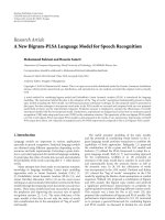
(a) Video frames captured from 4 different views
(b) Background images corresponding to each view
(c) Background subtraction results at each view
(d) Projection of detected points onto synthetic top view of ground-plane
Figure 3: Use of geometry in multiview detection: (a) snapshot from each view, (b) object free background image, (c) background
subtraction results, (d) synthetically generated top view of the ground plane. The bottom point (feet) of each blob is mapped to the ground
plane using the image-plane to ground-plane homography. Each color represents a blob detected in a different camera view. Points of
different colors very close together on the ground plane probably correspond to the same subject seen via different camera views.
where Ω

t
is a zero mean noise process with an identity
covariance matrix. Λ(x
t
) sets the covariance matrix of the
overall noise and is defined as
Λ
(
x
t
)
=
⎡
⎢
⎢
⎢
⎢
⎣
Σ
1
x
(
x
t
)
··· 0
2×2
.
.
.

.
.
.
.
.
.
0
2×2
··· Σ
M
x
(
x
t
)
⎤
⎥
⎥
⎥
⎥
⎦
1/2
,(4)
where 0
2×2
is a 2× 2matrixwithzeroforallentries.Σ
i
x
(x
t

)is
the covariance matrix associated with the transformation H
i
,
andisdefinedas
Σ
i
x
(
x
t
)
= J
H
i
(
x
t
)
S
u
J
H
i
(
x
T
)
,
(5)

where S
u
= diag[σ
2
, σ
2
], and J
H
i
(x
t
) is the Jacobian of the
transformation defined in (1).
EURASIP Journal on Image and Video Processing 5
The observation model in (3) is a multiview complete
observer model. There are two important features that this
model captures.
(i) The noise properties of the observations from differ-
ent views are different, and the covariances depend
not only on the view, but also on the true location of
the target x
t
. This dependence is encoded in Λ.
(ii) The MLE of x
t
(i.e., the value of x
t
that maximizes
the probability p(y
t

| x
t
)) is a minimum variance
estimator.
Tracking of target(s) is performed using a particle
filter [15]. This algorithm can be easily implemented in a
distributed sensor network. Each camera transmits the blobs
extracted from the background subtraction algorithm to
other nodes in the network. For the purposes of tracking, it is
adequate even if we approximate the blob with an enclosing
bounding box. Each camera maintains a multiobject tracker
filtering the outputs received from all the other nodes (along
with its own output). Further, the data association problem
between the tracker and the data is solved at each node
separately and the association with maximum likelihood is
transmitted along with data to other nodes.
3. Activity Modeling and
Recognition from Multiple Vi ews
As targets are tracked using multiview inputs, we need
to identify the activity performed by them. Given that
the tracking algorithm is preceded by a data association
algorithm, we can analyze the activity performed by each
individual separately. As targets are tracked, we associate
background subtracted silhouettes with each target at each
time instant and across multiple views. In the end, the
activity recognition is performed using multiple sequences
of silhouettes, one from each camera.
3.1. Linear Dynamical System for Activity Modeling. In
several scenarios (such as far-field surveillance and objects
moving on a plane), it is reasonable to model constant

motion in the real world using a linear dynamic system
(LDS) model on the image plane. Given P +1consecutive
video frames s
k
, , s
k+P
,let f (i) ∈ R
n
denote the obser-
vations (silhouette) from that frame. Then, the dynamics
during this segment can be represented as
f
(
t
)
= Cz
(
t
)
+ w
(
t
)
, w
(
t
)
∼ N
(
0, R

)
,
(6)
z
(
t +1
)
= Az
(
t
)
+ v
(
t
)
, v
(
t
)
∼ N
(
0, Q
)
,
(7)
where z
∈ R
d
is the hidden state vector, A ∈ R
d×d

the
transition matrix, and C
∈ R
n×d
the measurement matrix. w
and v are noise components modeled as normal with 0 mean
and covariance R and Q, respectively. Similar models have
been successfully applied in several tasks such as dynamic
texture synthesis and analysis [19], comparing silhouette
sequences [20, 21], and video summarization [22].
3.2. Learning the LTI Models for Each Segment. As described
earlier, each segment is modeled as an linear time invariant
(LTI) system. We use tools from system identification to
estimate the model parameters for each segment. The most
popular model estimation algorithms is PCA-ID [19]. PCA-
ID [19] is a suboptimal solution to the learning problem. It
makes the assumption that filtering in space and time are
separable, which makes it possible to estimate the parameters
of the model very efficiently via principal component analysis
(PCA).
We briefly describe the PCA-based method to learn the
model parameters here. Let observations f (1), f (2), , f (τ)
represent the features for the frames 1, 2, ,τ.Thegoal
is to learn the parameters of the model given in (7). The
parameters of interest are the transition matrix A and the
observation matrix C.Let[f (1), f (2), , f (τ)]
= UΣV
T
be the singular value decomposition of the data. Then,
the estimates of the model parameters (A, C)aregiven

by

C = U,

A = ΣV
T
D
1
V(V
T
D
2
V)
−1
Σ
−1
,whereD
1
=
[0 0; I
τ−1
0] and D
2
= [I
τ−1
0; 0 0]. These estimates of C and
A constitute the model parameters for each action segment.
For the case of flow, the same estimation procedure is
repeated for the x-andy-components of the flow separately.
Thus, each segment is now represented by the matrix pair

(A, C).
3.3. Classification of Actions. In order to perform classifica-
tion, we need a distance measure on the space of LDS models.
Several distance metrics exist to measure the distance
between linear dynamic models. A unifying framework based
on subspace angles of observability matrices was presented
in [23] to measure the distance between ARMA models.
Specific metrics such as the Frobenius norm and the Martin
metric [24] can be derived as special cases based on the
subspace angles. The subspace angles (θ
1
, θ
2
, ) between the
range spaces of two matrices A and B are recursively defined
as follows [23]:
cos θ
1
= max
x,y


x
T
A
T
By


Ax

2


By


2
=



x
T
1
A
T
By
1



Ax
1

2


By
1



2
,
cos θ
k
= max
x,y


x
T
A
T
By


Ax
2


By


2
=



x
T

k
A
T
By
k



Ax
k

2


By
k


2
for k = 2, 3, ,
(8)
subject to the constraints x
T
i
A
T
Ax
k
= 0andy
T

i
B
T
By
k
= 0for
i
= 1, 2 , k − 1. The subspace angles between two ARMA
models [A
1
, C
1
, K
1
]and[A
2
, C
2
, K
2
]canbecomputedby
the method described in [23]. Efficient computation of the
angles can be achieved by first solving a discrete Lyapunov
equation, for details of which we refer the reader to [23].
Using these subspace angles θ
i
, i = 1, 2, , n, three distances,
Martin distance (d
M
), gap distance (d

g
), and Frobenius
6 EURASIP Journal on Image and Video Processing
distance (d
F
) between the ARMA models are defined as
follows:
d
2
M
= ln
n

i=1
1
cos
2
(
θ
i
)
, d
g
= sin θ
max
, d
2
F
= 2
n


i=1
sin
2
θ
i
.
(9)
We use the Frobenius distance in all the results shown
in this paper. The distance metrics defined above cannot
account for low-level transformation such as when there is
a change in viewpoint or there is an affine transformation of
the low-level features. We propose a technique to build these
invariances into the distance metrics defined previously.
3.4. Affine and View Invariance. In our model, under feature
level affine transforms or view-point changes, the only
change occurs in the measurement equation and not the
state equation. As described in Section 3.2 the columns of
the measurement matrix (C) are the principal components
(PCs) of the observations of that segment. Thus, we need
to discover the transformation between the corresponding C
matrices under an affine/view change. It can be shown that
under affine transformations the columns of the C matrix
undergo the same affine transformation [22].
Modified Distance Metric. Proceeding from the above, to
match two ARMA models of the same activity related by a
spatial transformation, all we need to do is to transform the
C matrices (the observation equation). Given two systems
S
1

= (A
1
, C
1
)andS
2
= (A
2
, C
2
) we modify the distance
metric as

d
(
S
1
, S
2
)
= min
T
d
(
T
(
S
1
)
, S

2
)
, (10)
where d(
·, ·) is any of the distance metrics in (9), T is the
transformation. T(S
1
) = (A
1
, T(C
1
)). Columns of T(C
1
)are
the transformed columns of C
1
. The optimal transformation
parameters are those that achieve the minimization in (10).
The conditions for the above result to hold are satisfied by
the class of affine transforms. For the case of homographies,
the result is valid when it can be closely approximated by
an affinity. Hence, this result provides invariance to small
changes in view. Thus, we augment the activity recognition
module by examples from a few canonical viewpoints. These
viewpoints are chosen in a coarse manner along a viewing
circle.
Thus,foragivensetofactionsA
={a
i
},westorea

few exemplars taken from different views V
={V
j
}.After
model fitting, we have the LDS parameters for S
(i)
j
for action
a
i
from viewing direction V
j
. Given a new video, the action
classification is given by


i,

j

=
min
i,j

d

S
test
, S
(

i
)
j

,
(11)
where

d(·, ·)isgivenby(10).
We also need to consider the effect of different execution
rates of the activity when comparing two LDS parameters.
In the general case, one needs to consider warping functions
of the form g(t)
= f (w(t)) such as in [25] where Dynamic
time warping (DTW) is used to estimate w(t). We consider
linear warping functions of the form w(t)
= qt for each
action. Consider the state equation of a segment: X
1
(k) =
A
1
X
1
(k − 1) + v(k). Ignoring the noise term for now, we
can write X
1
(k) = A
k
1

X(0). Now, consider another sequence
that is related to X
1
by X
2
(k) = X
1
(w(k)) = X
1
(qk). In
the discrete case, for noninteger q thisistobeinterpreted
as a fractional sampling rate conversion as encountered in
several areas of DSP. Then, X
2
(k) = X
1
(qk) = A
qk
1
X(0), that
is, the transition matrix for the second system is related to
the first by A
2
= A
q
1
. Given two transition matrices of the
same activity but with different execution rates, we can get
an estimate of q from the eigenvalues of A
1

and A
2
as
q =

i
log



λ
(i)
2




i
log



λ
(i)
1



, (12)
where λ

(i)
2
and λ
(i)
1
are the complex eigenvalues of A
2
and
A
1
,respectively.Thus,wecompensatefordifferent execution
rates by computing
q. After incorporating this, the distance
metric becomes

d
(
S
1
, S
2
)
= min
T,q
d
(
T

(
S

1
)
, S
2
)
,
(13)
where T

(S
1
) = (A
q
1
, T(C
1
)). To reduce the dimensionality
of the optimization problem, we can estimate the time-warp
factor q and the spatial transformation T separately.
3.5. Inference from Multiview Sequences. In the proposed
system, each moving human can potentially be observed
from multiple cameras, generating multiple observation
sequences that can be used for activity recognition (see
Figure 4). While the modified distance metric defined in
(10)allowsforaffine view invariance and homography
transformations that are close to affinity, the distance metric
does not extend gracefully for large changes in view. In this
regard, the availability of multiview observations allow for
the possibility that the pose of the human in one of the
observations is in the vicinity of the pose in the training

dataset. Alternatively, multiview observations reduce the
range of poses over which we need view invariant matching.
In this paper, we exploit multiview observations by matching
each sequence independently to the learnt models and
picking the activity that matches with the lowest score.
After activity recognition is performed, an index of
the spatial locations of the humans and the activity that
is performed over various time intervals is created. The
visualization system renders a virtual scene using a static
background overlaid with virtual actors animated using the
indexed information.
4. Visualization and Rendering
The visualization subsystem is responsible for synthesizing
the output of all of the other subsystems and algorithms and
transforming them into a unified and coherent user experi-
ence. The nature of the data managed by our system leads
EURASIP Journal on Image and Video Processing 7
Training set
Pick Squat Bend Phone Throw
View 1
View 2
Te s t
Best view
and action
Recognize action and
visualize
Figure 4: Exemplars from multiple views are matched to a test sequence. The recognized action and the best view are then used for synthesis
and visualization.
to a somewhat unorthodox user interaction model. The user
is presented with a 3D reconstruction of the target scenario

as well as the acquired videos. The 3D reconstruction and
video streams are synchronized and are controlled by the user
via the navigation system described in what follows. Many
visualization systems deal with spatial data, allowing six
degrees of freedom, or temporal data, allowing two degrees
of freedom. However, the visualization system described here
allows the user eight degrees of freedom, as they navigate the
reconstruction of various scenarios.
For spatial navigation, we employ a standard first per son
interface where the user can move freely about the scene.
However, to allow for broader views of the current visualiza-
tion, we do not restrict the user to a specific height above the
ground plane. In addition to unconstrained navigation, the
user may choose to view the current visualization from the
vantage point of any of the cameras that were used during the
acquisition process. Finally, the viewpoint may be smoothly
transitioned between these different vantage points; a process
made smooth and visually appealing through the use of
double quaternion interpolation [26].
Temporal navigation employs a DVR-like approach.
Users are allowed to pause fast forward and rewind the
ongoing scenario. The 3D reconstruction and video display
actually run in different client applications, but maintain
synchronization via message passing. The choice to decouple
the 3D and 2D components of the system was made to allow
for greater scalability and is discussed in more detail below.
The design and implementation of the visualization
system is driven by numerous requirements and desiderata.
Broadly, the goals for which we aim are scalability and visual
fidelity. More specifically, they can be enumerated as follows.

(1) Scalability
(i) system should scale well across a wide range
of display devices, such as a laptop to a tiled
display,
(ii) system should scale to many independent
movers,
(iii) integration of new scenarios should be easy.
(2) Visual fidelity
(i) visual fidelity should be maximized subject to
scalability and interactivity considerations,
(ii) environmental effects impact user perception
and should be modeled,
(iii) when possible (and practical) the visualization
should reflect the appearance of movers,
(iv) coherence between the video and the 3D
visualization mitigate cognitive dissonance, so
discrepancies should be minimized.
4.1. Scalability and Modularity. The initial target for the
visualization engine was a cluster with 15 CPU/GPU coupled
display nodes. The general architecture of this system is illus-
trated in Figure 5(a), and an example of the system interface
running on the tiled display is shown in Figure 5(b). This
cluster drives a tiled display of high resolution LCD monitors
with a combined resolution of 9600
× 6000 for a total of
57 million pixels. All nodes are connected by a combination
Infiniband/Myrinet network as well as gigabit ethernet.
To speed development time and avoid some of the
more mundane details involved in distributed visualization,
we built the 3D component atop OpenSG [27, 28]. We

meet our scalability requirement by decoupling the disparate
components of the visualization and navigation system as
much as possible. In particular, we decouple the renderer,
which is implemented as a client application, from the user
input application, which acts as a server. On the CPU-
GPU cluster, this allows the user to directly interact with a
control node from which the rendering nodes operate inde-
pendently, but from which they accept control over viewing
and navigation parameters. Moreover, we decouple the 3D
visualization, which is highly interactive in nature, from the
2D visualization, which is essentially noninteractive. Each
video is displayed in a separate instance of the MPlayer
application. An additional client program is coupled with
each MPlayer instance, which receives messages sent by the
user input application over the network and subsequently
controls the video stream in accordance with these messages.
The decoupling of these different components serves dual
8 EURASIP Journal on Image and Video Processing
RAID
array
Storage nodes
C
P
U
C
P
U
C
P
U

C
P
U
Compute nodes
C
P
U
C
P
U
GPU
C
P
U
C
P
U
GPU
C
P
U
C
P
U
GPU
C
P
U
C
P

U
GPU
Display nodes
C
P
U
C
P
U
GPU
C
P
U
C
P
U
GPU
C
P
U
C
P
U
GPU
C
P
U
C
P
U

GPU
Infiniband network
10 Gb ethernet
User displays
Tiled display
(a) CPU-GPU cluster architecture (b) The visualization system running on the cluster
Figure 5: The visualization system was designed with scalability as a primary goal. It is a diagram of the general system architecture (a) as
well as a shot of the system running on the LCD tiled display wall (b).
Scenario 1
Position data
Scene
description
.
.
.
Scenario N
Position data
Scene
description
Geometry
database
(a)
123 N

Walk Throw

(b)
Figure 6: The sharing of data enhances the scalability of the
system. (a) illustrates how geometry is shared among multiple proxy
actors, while (b) illustrates the sharing of composable animation

sequences.
goals. First, it facilitates scaling the number of systems
participating in the visualization trivial. Second, reducing
interdependence among components allows for superior
performance.
This modularization extends from the design of the
rendering system to that of the animation system. In fact,
scenario integration is nearly automatic. Each scenario has a
unique set of parameters (e.g., number of actors, actions per-
formed, duration), and a small amount of meta-data (e.g.,
location of corresponding videos and animation database),
and is viewed by the rendering system as a self-contained
package. Figure 6(a) illustrates how each packaged scenario
interacts with the geometry database, which contains models
and animations for all of the activities supported by the
system. The position data specifies a location, for each frame,
for all of the actors tracked by the acquisition system. The
scene description data contains information pertaining to the
activities performed by each actor for various frame ranges
as well as the temporal resolution of the acquisition devices
(this latter information is needed to keep the 3D and 2D
visualizations synchronized).
The requirement that the rendering system should scale
to allow many actors dictates that shared data must be
exploited. This data sharing works at two distinct levels. First,
geometry is shared. The targets tracked in the videos are
represented in the 3D visualization by representative proxy
models, both because the synchronization and resolution of
the acquisition devices prohibit stereo reconstruction, and
because unique and detailed geometry for every actor would

constitutetoomuchdatatobeefficiently managed in our
distributed system. This sharing of geometry means that the
proxy models need not to be loaded separately for each actor
in a scenario, thereby reducing the system and video card
memory footprint. The second level at which data is shared is
at the animation level. This is illustrated in Figure 6(b).Each
animation consists of a set of keyframe data, describing one
iteration of an activity. For example, two steps of the walking
animation bring the actor back into the original position.
Thus, the walking animation may be looped, while changing
the actor’s position and orientation, to allow for longer
sequences of walking. The other animations are similarly
composable. The shared animation data means that all of the
characters in a given scenario who are performing the same
activity may share the data for the corresponding animation.
If all of the characters are jogging, for instance, only one copy
of the jogging animation needs to reside in memory, and
each of the performing actors will access the keyframes of
this single, shared animation.
4.2. Visual Fidelity. Subject to the scalability and interactivity
constraints detailed above, we pursue the goal of maximizing
the visual fidelity of the rendering system. Advanced visual
effects serve not only to enhance the experience of the user,
butoftentoprovidenecessaryandusefulvisualcuesand
to mitigate distractions. Due to the scalability requirement,
each geometry proxy is of relatively low polygonal complex-
ity. However, we use smooth shading to improve the visual
fidelity of the resulting rendering.
EURASIP Journal on Image and Video Processing 9
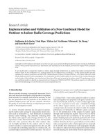
(a) (b)

Figure 7: Shadows add a significant visual realism to a scene as well as enhance the viewer’s perception of relative depth and position. Above,
the same scene is rendered without shadows (a) and with shadows (b).
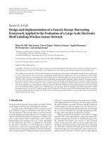
(a)
(b)
(c)
Figure 8: Several different environmental effects implemented in the rendering system. (a) shows a haze induced atmospheric scattering
effect. (b) illustrates the rendering of rain and a wet ground plane. (c) demonstrates the rendering of the same scene at night with multiple
local illumination sources.
Other elements, while still visually appealing, are more
substantive in what they accomplish. Shadows, for example,
have a significant effect on the viewer’s perception of depth
and the relative locations and motions of objects in a
scene [29]. The rendering of shadows has a long history
in computer graphics [30]. OpenSG provides a number
of shadow rendering algorithms, such as variance shadow
maps [31] and percentage closer filtering shadow maps [32].
We use variance shadow maps to render shadows in our
visualization, and the results can be seen in Figure 7.
Finally, the visualization system implements the render-
ing of a number of environmental effects. In addition to
generally enhancing the visual fidelity of the reconstruction,
these environmental effects serve a dual purpose. Differences
between the acquired videos and the 3D visualization can
lead the user to experience a degree of cognitive dissonance.
If, for example, the acquired videos show rain and an overcast
sky while the 3D visualization shows a clear sky and bright
sun, this may distract the viewer, who is aware that the
visualization and videos are meant to represent the same
scene, yet they exhibit striking visual differences. In order
to ameliorate this effect, we allow for the rendering of a

number of environmental effects which might be present
during video acquisition. Figure 8 illustrates several different
environmental effects.
5. Results
We tested the described system on the outdoor camera
facility at the University of Maryland. Our testbed consists
of six wall-mounted Pan Tilt Zoom cameras observing
an area of roughly 30 m
× 60 m. We built a static model
of the scene using simple planar structures and manually
aligned high resolution textures on each surface. Camera
locations and calibrations were done manually by registering
points on their image plane with respect to scene points
and using simple triangulation techniques to obtain both
their internal and external parameters. Finally, the image
plane to scene plane transformation were computed by
defining a local coordinate system on the ground plane and
using manually obtained correspondences to compute the
projective transformation linking the two.
5.1. Multiview Tracking. We tested the efficiency of the
multicamera tracking system over a four camera system. (see
Figure 9). Ground truth was obtained using markers on the
10 EURASIP Journal on Image and Video Processing
(a)
0
50
100
150
200
1000 2000 3000 4000 5000 6000 7000 8000

0
50
100
150
200
1000 2000 3000 4000 5000 6000 7000 8000
0
100
200
300
400
1000 2000 3000 4000 5000 6000 7000 8000
Frame number
Isotropic observation model
Proposed observation model
(b)
Figure 9: Tracking results for three targets over the 4 camera dataset. (best viewed in color/at high Zoom) (a) Snapshots of tracking output at
various timestamps. (b) Evaluation of tracking using Symmetric KL divergence from ground truth. Two systems are compared: one using the
proposed observation model and the other using isotropic models across cameras. Each plot corresponds to a different target. The trackers
using isotropic models swap identities around frame 6000. The corresponding KL-divergence values go off scale.
(a)
(b)
Figure 10: Output from the multiobject tracking algorithm working with input from six camera views. (a) Shows four camera views of a
scene with several humans walking. Each camera independently detects/tracks the humans using a simple background subtraction scheme.
The center location of the feet of each human is indicated with color-coded circles in each view. These estimates are then fused together
taking into account the relationship between each view and the ground plane. (b) shows the fused trajectories overlaid on a top-down view
of the ground plane.
EURASIP Journal on Image and Video Processing 11
Table 1: Recognition experiment simulated view change data on the UMD database. The table shows a comparison of recognition
performance using (a) baseline technique—direct application of system distance, (b) center of mass heuristic, (c) proposed compensated

distance metric.
Activity
Baseline CMH Compensated distance
Exemplars Exemplars Exemplars
1101101 10
PickUpObject40 0 404040 50
Jog in Place 0 0 0 10 70 80
Push 0 0 20 40 10 20
Squat 4030 102030 60
Wave 30 30 40 20 40 40
Kick 10 0 405030 50
Bend to the side 0 10 0 30 30 70
Throw 0 10 30 40 0 40
TurnAround 0 40 202030 70
Talk on Cellphone 0 0 10 20 40 40
Average 1212 212932 52
(Squat)
(Jog-in-place)
(a)
Squat
Pick
object
Jog
Throw
Kick
Stand
0 100 200 300 400 500 600 700 800 900 1000
Frame number
Recognized action
Ground truth

(b)
Figure 11: Activity recognition results over a sequence involving a
single human performing various activities. (a) The two rows show
the sample silhouettes from the observation sequence. Also marked
in bounding boxes are detected activities: squat (in broken cyan)
and jogging-in-place (dark brown). The plot in (b) shows results of
activity detections over the whole video sequence. The related input
and rendered sequence have been provided in the supplementary
material available online at doi:10.1155/2009/259860.
plane, and manually annotating time-instants when subjects
reached the markers. In our experiments, we compare two
observation models, one employing the proposed approach
and the other that assumes isotropic modeling across views.
A particle filter was used to track, the choice motivated given
missing data points due to occlusion. Testing was performed
over a video of 8000 frames with three targets introduced
sequentially at frames 1000, 4300, and 7200. Figure 9 shows
tracking results for this experiment. The proposed model
consistently results in lower KL divergence to the ground
truth.
Figure 10 shows localization results of nine subjects over
the ground plane using inputs from six cameras. The subjects
were allowed to move around freely and the multicamera
algorithm described in this paper was used to track them.
The use of six cameras allowed for near complete coverage
of the sensed region, as well as coverage from multiple
cameras in many regions. The availability of multiview
observations allows us to obtain persistent tracking results
even under occlusion and poor background subtraction.
Finally, multiview fusion leads to robust estimate of the target

location.
5.2. Activity Analysis. Figure 11 shows recognition of activ-
ities of an individual performing activities using a single
camera. The observation sequence obtained for this scenario
was processing using a sliding window of 40 frames. For each
window of observations, LDS parameters were estimated
using the learning algorithm in Section 3.2. This is compared
against the parameters of the training sequences for the
various activities using the modified distance metric of (11).
We also designed recognition experiments to test the
ability of our approach to handle view invariances. In this
experiment, we have 10 activities—Bend, Jog, Push, Squat,
Wave, Kick, Batting, Throw, Turn Sideways, Pick Phone.Each
activity is executed at varying rates. For each activity, a model
12 EURASIP Journal on Image and Video Processing
(a) (b)
(c) (d)
Figure 12: Visualization of the multitarget tracking results of Figure 10. (a) and (c) with each image showing snapshots from four of the six
cameras. The proposed system allows for arbitrary placement of the virtual camera. We refer the reader to the supplementary material for a
video sequence showcasing this result.
(a) Squat
(b) Jog
Figure 13: Rendering of activities performed in Figure 11. What is
shown are snapshots of two activities as rendered by our system.
is learnt and stored as an exemplar. The features (flow-fields)
are then translated and scaled to simulate a camera shift and
zoom. Models were built on the new features, and tested
using the stored exemplars. For the recognition experiment,
we learnt only a single LDS model for the entire duration
of the activity instead of a sequence. We also implemented

a heuristic procedure in which affine transforms are com-
pensated for by locating the center of mass of the features
and building models around its neighborhood. We call it
Center of Mass Heuristic (CMH). Recognition percentages
are shown in Tab le 1 . The baseline column corresponds to
direct application of the Frobenius distance. We see that our
method performs better in almost all cases.
5.3. Visualization. Finally, the results of localization and
activity recognition are used in creating a virtual rendition
of the events of the videos. Figures 12 and 13 show snapshots
from the system working on the scenarios corresponding to
Figures 10 and 11. We direct the reader to videos in the
supplementary material that illustrate the results and the
tools of the proposed system.
6. Conclusion
In this paper, we present a test bed for novel visualization
of dynamic events of a scene by providing an end user the
freedom to view the scene from arbitrary points of view.
Using a sequence of localization and activity recognition
algorithms we index the dynamic content of a scene. The
captured information is rendered in the scene model using
virtual actors along with the tools to visualize the events
from arbitrary views. This allows the end user to get the
geometric and spatiotemporal relationships between events
and humans very intuitively. Future work involves modeling
complicated activities along with the ability to make the
rendered scene more faithful to the sensed imagery by
suitably tailoring the models used to drive the virtual
actors. Also of interest is providing a range of rendering
possibilities covering image-based rendering, virtual actors

and markerless motion capture methods. Such a solution
would require advance in both processing algorithms (such
EURASIP Journal on Image and Video Processing 13
as single view motion capture) and in rendering techniques
for fast visualization.
Acknowledgment
This work was supported by DARPA Flexiview Grant
HR001107C0059 and NSF CNS 04-03313.
References
[1] C F. Shu, A. Hampaour, M. Lu, et al., “IBM smart surveillance
system (S3): a open and extensible framework for event based
surveillance,” in Proceedings of IEEE International Conference
on Advanced Video and Signal Based Surveillance (AVSS ’05),
pp. 318–323, 2005.
[2] F. Porikli, “Multi-camera surveillance: object-based sum-
marization approach,” Tech. Rep. TR-2003-145, MERL A
Mitsubishi Electric Research Laboratory, March 2004.
[3] T. Kanade, R. Collins, A. Lipton, P. Burt, and L. Wixson,
“Advances in cooperative multi-sensor video surveillance,” in
Proceedings of DARPA Image Understanding Workshop, vol. 1,
pp. 3–24, 1998.
[4] A. Akbarzadeh, J. M. Frahm, P. Mordohai, et al., “Towards
urban 3D reconstruction from video,” in Proceedings of the 3rd
International Symposium on 3D Data Processing, Visualization,
and Transmission (3DPVT ’06), vol. 4, 2006.
[5] I. O. Sebe, J. Hu, S. You, and U. Neumann, “3D video surveil-
lance with augmented virtual environments,” in Proceedings of
International Multimedia Conference, pp. 107–112, ACM, New
York, NY, USA, 2003.
[6] T. Kanade and P.J. Narayanan, “Virtualized reality: perspec-

tives on 4D digitization of dynamic events,” IEEE Computer
Graphics and Applications, vol. 27, no. 3, pp. 32–40, 2007.
[7] J. Carranza, C. Theobalt, M. A. Magnor, and H P. Seidel,
“Free-viewpoint video of human actors,” ACM T ransactions on
Graphics, vol. 22, no. 3, pp. 569–577, 2003.
[8] G. Schindler, P. Krishnamurthy, and F. Dellaert, “Line-
based structure from motion for urban environments,” in
Proceedings of the 3rd International Symposium on 3D Data
Processing, Visualization, and Transmission (3DPVT ’06),pp.
846–853, 2006.
[9] G. Schindler, F. Dellaert, and S. B. Kang, “Inferring temporal
order of images from 3D structure,” in Proceedings of the IEEE
Computer Society Conference on Computer Vision and Pattern
Recognition (CVPR ’07), 2007.
[10] N. Snavely, S. M. Seitz, and R. Szeliski, “Photo tourism:
exploring photo collections in 3D,” in Proceedings of the 33rd
International Conference and Exhibition on Computer Graphics
and Interactive Techniques (SIGGRAPH ’06), pp. 835–846,
ACM Press, Boston, Mass, USA, July-August 2006.
[11] R. Hartley and A. Zisserman, Multiple View Geometry in
Computer V ision, Cambridge University Press, Cambridge,
UK, 2003.
[12] F. Fleuret, J. Berclaz, and R. Lengagne, “Multi-camera people
tracking with a probabilistic occupancy map,” Tech. Rep.
EPFL/CVLAB2006.07, July 2006.
[13] S. M. Khan and M. Shah, “A multi-view approach to
tracking people in crowded scenes using a planar homography
constraint,” in Proceedings of the 9th European Conference
on Computer Vision (ECCV ’06), vol. 4, pp. 133–146, Graz,
Austria, May 2006.

[14] K. Kim and L. S. Davis, “Multi-camera tracking and segmenta-
tion of occluded people on ground plane using search-guided
particle filtering,” in Proceedings of the 9th European Conference
on Computer Vision (ECCV ’06), vol. 3953 of Lecture Notes in
Computer Science, pp. 98–109, Graz, Austria, May 2006.
[15] A. C. Sankaranarayanan and R. Chellappa, “Optimal multi-
view fusion of object locations,” in Proceedings of IEEE
Workshop on Motion and Video Computing (WMVC ’08),pp.
1–8, Copper Mountain, Colo, USA, January 2008.
[16] B. D. O. Anderson and J. B. Moore, Optimal Filter ing,Dover,
New York, NY, USA, 2005.
[17] A. Doucet, N. D. Freitas, and N. Gordon, Sequential Monte
Carlo Methods in Practice, Springer, New York, NY, USA, 2001.
[18] Y. Bar-Shalom and T. Fortmann, Tracking and Data Associa-
tion, Academic Press, New York, NY, USA, 1988.
[19] S. Soatto, G. Doretto, and Y. N. Wu, “Dynamic textures,”
in Proceedings of the 8th IEEE International Conference on
Computer Vision (ICCV ’01), vol. 2, pp. 439–446, Vancouver,
Canada, July 2001.
[20] A. Veeraraghavan, A. K. Roy-Chowdhury, and R. Chellappa,
“Matching shape sequences in video with applications in
human movement analysis,” IEEE Transactions on Pattern
Analysis and Machine Intelligence, vol. 27, no. 12, pp. 1896–
1909, 2005.
[21] A. Bissacco, A. Chiuso, Y. Ma, and S. Soatto, “Recognition of
human gaits,” in Proceedings of IEEE Computer Society Confer-
ence on Computer Vision and Pattern Recognition (CVPR ’01),
vol. 2, pp. 52–57, December 2001.
[22] P. Turaga, A. Veeraraghavan, and R. Chellappa, “Unsupervised
view and rate invariant clustering of video sequences,” Com-

puter Vision and Image Understanding, vol. 113, no. 3, pp. 353–
371, 2009.
[23] K. De Cock and B. De Moor, “Subspace angles between ARMA
models,” Systems and Control Letters, vol. 46, no. 4, pp. 265–
270, 2002.
[24] R. J. Martin, “A metric for ARMA processes,” IEEE Transac-
tionsonSignalProcessing, vol. 48, no. 4, pp. 1164–1170, 2000.
[25] A. Veeraraghavan, R. Chellappa, and A. K. Roy-Chowdhury,
“The function space of an activity,” in Proceedings of IEEE
Computer Society Conference on Computer Vision and Pattern
Recognition (CVPR ’06), vol. 1, pp. 959–966, 2006.
[26] Q. J. Ge, A. Varshney, J. Menon, and C. Chang, “Double
quaternions for motion interpolation,” in Proceedings of the
ASME Design Engineering Technical Conference,September
1998, DETC98/DFM-5755.
[27] D. Reiners, G. Voss, and J. Behr, “Opensg: basic concepts,”
in Proceedings of the 1st OpenSG Symposium (OpenSG ’02),
Darmstadt, Germany, 2002.
[28] D. Reiners, “Special issue on the OpenSG symposium and
OpenSG plus,” Computers & Graphics,vol.28,no.1,pp.59–
61, 2004.
[29] D. Kersten, D. C. Knill, P. Mamassian, and I. Bulthoff,“Illusory
motion from shadows,” Nature, vol. 379, no. 6560, p. 31, 1996.
[30] F. C. Crow, “Shadow algorithms for computer graphics,”
SIGGRAPH Computer Graphics, vol. 11, no. 2, pp. 242–248,
1977.
[31] W. Donnelly and A. Lauritzen, “Variance shadow maps,” in
Proceedings of the Symposium on Interactive 3D Graphics and
Games (I3D ’06), pp. 161–165, ACM, New York, NY, USA,
2006.

[32] S. Brabec and H P. Seidel, “Hardware-accelerated rendering
of antialiased shadows with shadow maps,” in Proceedings of
the International Conference on Computer Graphics,H.H S.
Ip, N. Magnenat-Thalmann, R. W. H. Lau, and T S. Chua,
Eds., pp. 209–214, Hong Kong, July 2001.