báo cáo hóa học:" Research Article Random Bit Flipping and EXIT Charts for Nonuniform Binary Sources and Joint Source-Channel Turbo Systems" docx

Hindawi Publishing Corporation
EURASIP Journal on Advances in Signal Processing
Volume 2009, Article ID 354107, 6 pages
doi:10.1155/2009/354107
Research Article
Random Bit Flipping and EXIT Charts for Nonuniform Binary
Sources and Joint Source-Channel Turbo Systems
Xavier Jaspar
1
and Luc Vandendorpe
2
1
Laborelec, Rodestraat 125, B-1630 Linkebeek, Belgium
2
Communications and Remote Sensing Laboratory, Universit
´
e catholique de Louvain, Place du Levant 2,
B-1348 Louvain-la-Neuve, Belgium
Correspondence should be addressed to Xavier Jaspar,
Received 29 January 2009; Revised 7 June 2009; Accepted 7 August 2009
Recommended by Athanasios Rontogiannis
Joint source-channel turbo techniques have recently been explored a lot in literature as one promising possibility to lower the
end-to-end distortion, with fixed length codes, variable length codes, and (quasi) arithmetic codes. Still, many issues remain to
be clarified before production use. This short contribution clarifies very concisely several issues that arise with EXIT charts and
nonuniform binary sources (a nonuniform binary source can be the result of a nonbinary source followed by a binary source code).
We propose two histogram-based methods to estimate the charts and discuss their equivalence. The first one is a mathematical
generalization of the original EXIT charts to nonuniform bits. The second one uses a random bit flipping to make the bits virtually
uniform and has two interesting advantages: (1) it handles straightforwardly outer codes with an entropy varying with the bit
position, and (2) it provides a chart for the inner code that is independent of the outer code.
Copyright © 2009 X. Jaspar and L. Vandendorpe. This is an open access article distributed under the Creative Commons
Attribution License, which permits unrestricted use, distribution, and reproduction in any medium, provided the original work is

properly cited.
1. Introduction
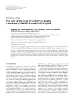
Consider the generic system in Figure 1.Itinvolvesaserial
concatenation at the transmitter and a joint source-channel
serial turbo decoder [1, 2] at the receiver and is sufficiently
general to describe several issues that arise with EXIT charts
[3] when the bits U
:
are not uniform.
Let us consider that the outer component in Figure 1 is
a discrete source of symbols followed by a source code that
produces a sequence of Nbiased or nonuniform bits U
1:N
or
U
:
. After random interleaving by Π, the inner component
is a channel code that produces a sequence of coded bits
R
:
which are sent across the channel. We assume that the
channel code is linear and the channel is binary, symmetric,
memoryless, and time invariant. At the receiver, an iterative
decoder is used, based on two decoders, one for each code.
They exchange log-likelihood ratios (LLRs) iteratively, in a
typical joint source-channel serial configuration [1, 2]. In the
following, let L
s
O,:
be the output LLRs of the (outer) source

decoder, let L
c
O,:
be the deinterleaved output LLRs of the
(inner) channel decoder, and let L
c
I,:
= L
s
O,:
and L
s
I,:
= L
c
O,:
be the corresponding input LLRs.
To assess the convergence of this iterative decoder, the
EXITchartsintroducedin[3] can be used when the bits
are uniform. Unfortunately, when the bits are not uniform,
a naive application of the EXIT charts that would neglect
the bias might lead to inaccuracy issues. A few contributions
already paid attention to some of these issues, notably [2, 4,
5]. This paper attempts to clarify them all.
This short paper presents concisely two simple
histogram-based techniques in Section 2 to estimate
the EXIT charts when the bits are not uniform and discusses
in Section 3 the (dis)advantages of each. The first technique
is based on the system in Figure 1 and is a generalization
of [5]; the second one is based on the system in Figure 2

where a random bit flipping is introduced. These techniques
are shown to lead to different but equivalent charts under
some assumptions. At last, we show that the well-known
technique in [6], though historically developed for uniform
bits, provides “correct” EXIT charts with nonuniform bits,
which is an interesting conclusion for readers familiar
with this technique. Please note that, this paper relates
only to histogram-based computations of EXIT charts but
2 EURASIP Journal on Advances in Signal Processing
Source
coder
U
:
Π
Channel
coder
R
:
Channel
Channel
decoder
L
s
I,:
= L
c
O,:
L
s
O,:

= L
c
I,:
Π
−1
Π
Y
:
Source
decoder
Figure 1: Generic joint source-channel turbo system.
Source
coder
U
:
U

:
Π
Channel
coder
R

:
Channel
Channel
decoder
Π
−1
L

c
O,:
L
s
O,:
Π
Y

:
Source
decoder
F
:
Flipped source (de)coder
Figure 2: Equivalent system with a random bit flipping,
U
k
, U

k
, F
k
∈{+1,−1}.AsinFigure 1, we define L
s
I,:
= L
c
O,:
and
L

s
O,:
= L
c
I,:
.
the presented ideas and concepts are compatible with the
analytical computation proposed in [7].
In the remainder, random variables are written with
capital letters and realizations with small letters. P(z) is the
abbreviation of the probability P(Z
= z). The subsequence
(Z
m
, Z
m+1
, , Z
n
)iswrittenZ
m:n
or Z
:
when m, n can be
omitted.
I{a} is the indicator function, that is, I{a} equals 1
if a is true, 0 otherwise. E
{Z} is the expectation of Z. I(Y; Z)
is the mutual information between Y and Z. H(Z)
= I(Z; Z)
is the entropy of Z. H

b
(p) is the binary entropy function, that
is, H
b
(p) =−p log
2
(p) −(1 − p)log
2
(1 − p).
2. Computation of the EXIT Charts
The main results of this section are summarized in Ta ble 1.
For clarity, the first method of computation, which is based
on biased bits, is given the name BEXIT while the second one,
which is based on flipped bits, is called FEXIT. For the sake
of conciseness, some familiarity with [3] is assumed.
2.1. Assumptions, Notations, and Consistency. We assu me
that the channel code is linear and the channel is binary,
symmetric, memoryless, and time invariant. Besides, we
assume that the channel and source decoders, taken apart,
are optimal. Specifically, let R
c
k
= (Y
:
, L
c
I,1:k
−1
, L
c

I,k+1:N
)and
R
s
k
= (L
s
I,1:k
−1
, L
s
I,k+1:N
), and assume that the elements in R
c
k
and in R
s
k
are independent, then the output LLRs on U
k
of
the channel and source decoders in Figure 1 are considered
to be, respectively,
L
c
O,k
= log
p

R

c
k
| U
k
= +1

p

R
c
k
| U
k
=−1

,(1)
L
s
O,k
= log
p

R
s
k
, U
k
= +1

p


R
s
k
, U
k
=−1

=
log
p

R
s
k
| U
k
= +1

p

R
s
k
| U
k
=−1

+ L
U,k

,
(2)
where the source bias L
U,k
is defined as
L
U,k
 log
P
(
U
k
= +1
)
P
(
U
k
=−1
)
,with0<P
(
U
k
= +1
)
< 1. (3)
Note that in the flipped case in Section 2.3, L

U,k

= 0. Note
also generalizing the results below to P(U
k
= +1) ∈{0, 1}
(e.g., in the case of pilot bits) is straightforward by taking the
limit of
|L
U,k
| toward infinity where appropriate.
To avoid any confusion, here are some further consider-
ations. Firstly, we prefer not to use the term “extrinsic” for
the LLRs L
c
O,k
and L
s
O,k
because this term is used differently
by authors in literature. Some authors consider these L
c
O,k
and L
s
O,k
in (1)-(2) as extrinsic; others consider L
c
O,k
(with
Y
k

excluded in the case of a systematic channel code) and
L
s
O,k
− L
U,k
as extrinsic. Secondly, we consider a typical
serial concatenation where only the (inner) channel decoder
has access to the channel values. It must therefore share
this piece of information with the source decoder through
L
c
O,k
.ThisiswhyL
c
O,k
in (1) depends on all channel values
Y
:
through R
c
k
(even if the channel code is systematic).
Similarly, only the (outer) source decoder “knows” the source
a priori probabilities. This is why, to share it with the channel
decoder, the source bias L
U,k
is included in L
s
O,k

in (2).
Definition 1 (P-consistency and L-consistency). L
p
is
posterior- consistent or P-consistent with U if
p
(
L
P
= l, U = +1
)
= e
l
p
(
L
P
= l, U =−1
)
. (4)
L
L
is likelihood-consistent or L-consistent with U if
p
(
L
L
= l | U = +1
)
= e

l
p
(
L
L
= l | U =−1
)
.
(5)
Note that if L
L
is L-consistent, then L
L
+ L
U
is P-consistent.
Proposition 1. TheoutputLLRofthechanneldecoder,L
c
O,k
in (1), is L-consistent with U
k
. The output LLR of the source
decoder, L
s
O,k
in (2), is P-consistent with U
k
.
Proof. It follows from (1)-(2) and integration of p(R
c

k
| u
k
)
and p(R
s
k
| u
k
).
Note that when the symmetry condition p(L =−l | U =
+1) = p(L = l | U =−1) is satisfied, the consistency in
[4, 6] and the L-consistency (5) are equivalent.
EURASIP Journal on Advances in Signal Processing 3
Table 1: Summary of the two Monte-Carlo methods.
BEXIT charts: with biased bits, Figure 1
FEXIT charts: with flipped bits, Figure 2
Generation of the
input LLRs
Given a value of I
I
, μ
L
= J
−1
L
U
(I
I
)andN

L
∼
N (0, 2μ
L
),
For both channel and source codes, given
avalueofI

I
, μ

L
= J
−1
0
(I

I
)and
N

L
∼ N (0, 2μ

L
),
(I) L
s
I
= μ

L
U + N
L
,
(III) L

I
= μ

L
U

+ N

L
.
(II) L
c
I
= μ
L
U + N
L
+ L
U
,
Note, L

U
= 0.

where L
s
I
is L-consistent and L
c
I
is P-consistent.
Measurement of
the output
information for
consistent LLRs
If L
s
O
is P-consistent and L
c
O
is L-consistent, we
have
If L

O
is consistent, we have for both
channel and source codes
(IV)
I
s
O
= H
U

−E{log
2
(1 + e
−UL
s
O
)},
(VIII)
I

O
= 1 −E{log
2
(1 + e
−U

L

O
)},
(V)
= H
U
−E{H
b
(1/1+e
L
s
O
)},

(IX)
= 1 −E{H
b
(1/1+e
L

O
)}.
(VI)
I
c
O
= H
U
−E{log
2
(1 + e
−U
(
L
U
+L
c
O
)
)
}, Under some ergodic assumption, these
(VII)
= H
U

−E{H
b
(1/1+e
L
U
+L
c
O
)}.
expectations can be approached by time
averages as in [6].
Under some ergodic assumption, these expecta-
tions can be approached by time averages as in [6].
Note, L

U
= 0andH

U
= 1.
Link between
BEXIT charts and
FEXIT charts
Let I
I,s
O,c
be I
s
I
= I

c
O
, I
I,s
O,c
be I
s
I
= I
c
O
, I
I,c
O,s
be I
c
I
= I
s
O
, I
I,c
O,s
be I
c
I
= I
s
O
, then:

(X) I
I,s
O,c
≈ J
L
U
(J
−1
0
(I
I,s
O,c
)) ←→ I
I,s
O,c
≈ J
0
(J
−1
L
U
(I
I,s
O,c
)).
(XI) I
I,c
O,s
= I
I,c

O,s
−(1 −H
U
) ←→ I
I,c
O,s
= I
I,c
O,s
+(1−H
U
).
Let us assume that L
U
= L
U,k
is independent of k; that is,
the bits U
k
have the same entropy H
U
= H
U,k
 H
b
(P(U
k
=
+1)) independently of k. Let us then measure the input and
output levels of information as

I
= lim
N →+∞
1
N
N

k=1
I
(
U
k
; L
k
)
∈
[
0, H
U
]
,(6)
where (I, L
k
)is(I
c
I
, L
c
I,k
), (I

s
I
, L
s
I,k
), (I
c
O
, L
c
O,k
), or (I
s
O
, L
s
O,k
).
As in [3], we will compute the charts I
c
O
= T
c
(I
c
I
)and
I
s
O

= T
s
(I
s
I
) by feeding the decoders with input LLRs and
by measuring the level of output information.
Remark 1. The channel (resp., source) decoder will be fed
with input LLRs that are independent, P-consistent (resp., L-
consistent, in agreement with Proposition 1), and Gaussian.
Proposition 2. Let L

U
be equal to 0 if L is P-consistent with U,
and let it be equal to L
U
if L is L-consistent. Then
P
(
U
= u | L = l
)
=
1
1+e
−u(L

U
+l)
. (7)

Proof. It follows from (4)-(5)andfromP(U
= +1 | L =
l)+P(U =−1 | L = l) = 1.
2.2. BEXIT Charts, Figure 1: Biased Bits. We c an co mp ut e
the BEXIT charts of the system in Figure 1 by analytical
generalization of the original EXIT charts [3].
(1) Generating the input LLRs. Letusconsiderasequenceof
bits U
:
generated by the source coder and let us focus on one
of these bits, namely, U.GivenavalueI
I
= I
s
I
, the input
LLR L
s
I
on U is generated as in (I) in Ta ble 1,whereN
L
is
a centered Gaussian random variable of variance 2μ
L
and the
invertible function J
L
U
(·)isgivenby
J

L
U

μ

=
H
U
−

u∈{+1,−1}
P
(
U = u
)
·

+∞
−∞
e
−
(
ξ−μu
)
2
/(4μ)

4πμ
log
2


1+e
−u(L
U
+ξ)

dξ.
(8)
This L
s
I
in (I), Ta bl e 1, is L-consistent, in agreement with
Remark 1.
For the channel decoder, given a value I
I
= I
c
I
, the input
LLR L
c
I
on U is generated as in (II), Ta bl e 1.Comparedto
(I), Ta ble 1 , the constant term L
U
is necessary to make L
c
I
P-
consistent.

(2) Measuring the output information. Let us consider the
whole sequence of bits U
:
and the corresponding output
LLRs L
O,:
. For both decoders, we can measure the output
information by (6)with
I

U
k
; L
O,k

=
H
U
−E

log
2
1
P

U
k
| L
O,k



. (9)
This expression can be evaluated by approaching P(U
k
|
L
O,k
) with histogram measurements as in [3].
Assuming consistent LLRs makes things simpler. We can
indeed simplify (6)and(9) into (IV) and (VI) , Tab le 1 ,by
4 EURASIP Journal on Advances in Signal Processing
Proposition 2 and by (9). In addition, we can simplify (IV)
into (V) since
E

log
2

1+e
−UL
s
O

|
L
s
O

=


u∈{+1,−1}
P

U = u | L
s
O

log
2

1+e
−uL
s
O

=
H
b

1

1+e
L
s
O


=
H
b


1

1+e
−L
s
O


,
(10)
where P(U
= u | L
s
O
)isgivenin(7). Similarly, we can
simplify (VI) into (VII), Tab le 1 . Note that (IV), Tab l e 1,is
equivalent to [5, equation (4)] and is an extension of [6,
equation (4)].
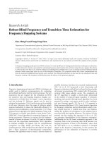
2.3. FEXIT Charts, Figure 2: Flipped Bits. Let us now consider
the system in Figure 2. To make the bit stream uniform, we
have introduced a random bit flipping before the interleaver
Π, that is, U

k
= U
k
F
k
for all k, where the F

k
∈{+1,−1}
are independent and uniformly distributed. At the receiver,
the corresponding LLRs are flipped accordingly. By linearity
of the channel code and symmetry of the channel, the
flipped system in Figure 2 is equivalent to the original system
in Figure 1. Consequently, the EXIT charts of the flipped
system, namely, FEXIT charts, can be used to characterize the
original system. For clarity, all symbols related to the flipped
system use a prime (

) notation.
With FEXIT charts, we are interested in the exchange
of information about U

:
between the channel decoder and
the flipped source decoder in Figure 2. Since the bits U

k
are uniform, we can use the results obtained so far with
L

U
= 0andH

U
= 1 (see Ta bl e 1). This is equivalent to [3];
in particular, the function J
0

(·) = J
L
U
=0
(·) is related to the
function J(
·)in[3]withJ
0
(μ

) = J(

2μ

).
3. Transformations, Equivalence,
and Discussion
3.1. Transformations and Equivalence. The BEXIT and
FEXIT charts are equivalent under the assumptions of
Section 2.1, up to the approximation (X), Ta bl e 1. Indeed,
under these assumptions, transformations to obtain the
FEXIT chart from the BEXIT chart, and vice versa, are given
in (X) and (XI) and Tab le 1.Toprove(X)andTa ble 1,let
us consider L
s
I
givenin(I),Tab le 1, in the biased case. If we
apply the flipping F on L
s
I

,wegetL
s
I
= L
s
I
F = μ
L
UF+N
L
F =
μ
L
U

+ N
L
F, and it is self-evident that this L
s
I
is equivalent
to (III), Ta ble 1,ifμ
L
= μ

L
, that is, if J
−1
L
U

(I
s
I
) = J
−1
0
(I
s
I
),
which proves (XI), Ta bl e 1, for consistent Gaussian LLRs. For
consistent non-Gaussian LLRs, we can invoke the empirical
robustness of EXIT charts with respect to the statistical
model of the LLRs and assume that (X), Ta bl e 1,isasufficient
approximation, hence the approximation symbol “
≈”. T o
prove (XI), Tabl e 1, we use the following equalities:
I
s
O
−H
U
=−E

log
2

1+e
−UL
s

O

,by
(
IV
)
, (11)
=−E

log
2

1+e
−U

L
s
O

, (12)
= I
s
O
−1, by
(
VIII
)
(13)
where (12) comes from U


L
s
O
= (UF)(L
s
O
F) = UL
s
O
.
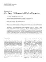
3.2. Simulation Results. To illustrate the equivalence, let us
compute the charts of the following (nonoptimized) system.
The outer component in Figure 1 isamemorylesssourceof
3 symbols with probabilities 0.85, 0.14, and 0.01, transcoded,
respectively, by the variable length codewords (+1), (
−1, −1),
(
−1, +1, −1), leading to P(U = +1) = 0.741 and H
U
=
0.825. The channel code is a rate −(1/2) recursive systematic
convolutional code with forward generator 35
8
(in octal) and
feedback generator 23
8
. The channel is an additive white
Gaussian noise channel with binary phase-shift keying and
E
b

/N
0
= 1.4dB—E
b
is the energy per bit of entropy and N
0
/2
the double-sided noise spectral density. Note that the source
decoder is based on the BCJR algorithm [8] on Balakirsky’s
bit-trellis [9].
The BEXIT and FEXIT charts of the system are given in
Figures 3 and 4. The solid lines show the charts obtained
with the methods described in Sections 2.2 and 2.3.The
data points show the BEXIT and FEXIT charts obtained by
applying the transformations (X)-(XI), Ta b le 1 ,respectively,
on the FEXIT and BEXIT charts given in solid lines. The good
match between the data points and the solid lines illustrates
the equivalence between FEXIT and BEXIT charts. All system
configurations we have tested confirm this equivalence, at
least in the tested range P(U
= +1) ∈ [0.05, 0.95].
Finally, when we neglect the bias and apply blindly the
original method of [3]—generating the input LLRs with [3,
equation (9)] and [3, equation (18)] and measuring the
output information with [3,equation(19)]—,weobtain
actually the FEXIT chart of the channel decoder for the
channel decoder and the dashed line in Figure 4 for the
source decoder. As we can see, these charts intersect each
other and give a prediction of convergence that is too
pessimistic.

3.3. Discussion. In terms of (dis)advantages of each method,
FEXIT charts, unlike BEXIT charts, are limited to linear
channel codes and symmetric channels. Nevertheless, when
the channel code is linear and the channel symmetric, FEXIT
charts have at least two benefits. Firstly, the FEXIT chart of
the (inner) channel code is independent of the (outer) source
code; so we do not need to recompute it when the source code
changes. By contrast, we need to recompute the BEXIT chart
of the channel code when L
U
changes since it depends on L
U
(see (II), (VI), and (VII) in Ta ble 1). Secondly, FEXIT charts
can handle very easily (outer) source codes with an entropy
H
U,k
that depends on k—recall that we have assumed that
L
U,k
, therefore H
U,k
, is independent of k in Section 2.1—,
simply because the random bit flipping makes the entropy
EURASIP Journal on Advances in Signal Processing 5
00.20.40.60.81
I
c
I
··· I
s

O
0
0.2
0.4
0.6
0.8
1
I
c
O
··· I
s
I
BEXIT charts
FEXIT charts, transformed
Figure 3: BEXIT charts of the system described in Section 3.1.
00.20.40.60.81
I
c
I
··· I
s
O
0
0.2
0.4
0.6
0.8
1
I

c
O
··· I
s
I
BEXIT charts
FEXIT charts, transformed
EXIT chart VLC, bias neglected
Figure 4: FEXIT charts of the system described in Section 3.1.
equal to 1 for all k. On the contrary, no method to handle
them with BEXIT charts is known to the authors. Note that
a varying H
U,k
is not uncommon in practice: fixed length
codes, variable length codes with periodic bit-clock trellises,
mixture of such codes, and so forth.
At last, among related contributions in literature, the
well-known technique in [6] is of particular interest. Though
historically developed for uniform bits, this technique gives
without bit flipping a correct prediction of convergence when
the channel code is linear and the channel is symmetric. It
computes indeed [6, equation (5)] the output information
as (with some mathematical rewriting)
I
[6]
O
= 1 −E

log
2


1+e
−UL

. (14)
Since U

L

= (UF)(LF) = UL, it is equivalent to (VIII),
Ta bl e 1, and thus to the FEXIT charts presented in this paper.
4. Conclusion
Two methods have been presented to handle nonuniform
bits in the computation of EXIT charts. Though proved
to be equivalent for the prediction of convergence under
certain assumptions, they have different pros and cons. For
example, the FEXIT method is restricted to linear inner
codes and symmetric channels while the BEXIT method is
not. But the FEXIT method handles very easily a mixture
of bits having different entropies and offers a chart for the
inner channel decoder (of a serial concatenation) that is
independent of the outer source code, unlike the BEXIT
method, which simplifies greatly subsequent optimizations
of the concatenated code. In practice, both methods are
therefore complementary and help to analyze joint source-
channel turbo systems via EXIT charts.
Acknowledgment
The authors greatly thank the reviewers for their constructive
comments. The work of X. Jaspar is supported by the F.R.S
FNRS, Belgium.

References
[1]A.Guyader,E.Fabre,C.Guillemot,andM.Robert,“Joint
source-channel turbo decoding of entropy-coded sources,”
IEEE Journal on Selected Areas in Communications, vol. 19, no.
9, pp. 1680–1696, 2001.
[2] M. Adrat and P. Vary, “Iterative source-channel decoding:
Improved system design using EXIT charts,” EURASIP Journal
on Applied Signal Processing, vol. 2005, no. 6, pp. 928–947, 2005.
[3] S. ten Brink, “Convergence behavior of iteratively decoded
parallel concatenated codes,” IEEE Transactions on Communi-
cations, vol. 49, no. 10, pp. 1727–1737, 2001.
[4] J. Hagenauer, “The EXIT chart—introduction to extrinsic
information transfer in iterative processing,” in Pro ceedings o f
the 12th European Signal Processing Conference (EUSIPCO ’04),
Vienna, Austria, September 2004.
[5] N. D
¨
utsch, “Code optimisation for lossless compression of
binary memoryless sources based on FEC codes,” European
Transactions on Telecommunications, vol. 17, no. 2, pp. 219–229,
2006.
[6] M. T
¨
uchler and J. Hagenauer, “EXIT charts of irregular codes,”
in Proceedings of the 36 th Annual Conference on Information
Sciences and Systems (CISS ’02), Princeton, NJ, USA, March
2002.
6 EURASIP Journal on Advances in Signal Processing
[7]M.Adrat,J.Brauers,T.Clevorn,andP.Vary,“TheEXIT-
characteristic of softbit-source decoders,” IEEE Communica-

tions Letters, vol. 9, no. 6, pp. 540–542, 2005.
[8] L. R. Bahl, J. Cocke, F. Jelinek, and J. Raviv, “Optimal decoding
of linear codes for minimizing symbol error rate,” IEEE
Transactions on Information Theory, vol. 20, no. 2, pp. 284–287,
1974.
[9] V. B. Balakirsky, “Joint source-channel coding with variable
length codes,” in Proceedings of the IEEE International Sympo-
sium on Information Theory (ISIT ’97), p. 419, Ulm, Germany,
July 1997.