Electric Machinery Fundamentals Power & Energy_2 potx

17

TOT stator air gap 1 rotor air gap 2
=+ ++RRR RR
At a flux density of 1.2 T, the relative permeability
r
µ
of the stator is about 3800, so the stator reluctance
is

()
()
()()
stator
stator
7
stator stator
0.48 m
62.8 kA t/Wb
3800 4 10 H/m 0.04 m 0.04 m
l
A
µ
π
−
== =⋅
×
R

At a flux density of 1.2 T, the relative permeability

r
µ
of the rotor is 3800, so the rotor reluctance is

()
()
()()
rotor
rotor
7
stator rotor
0.04 m
5.2 kA t/Wb
3800 4 10 H/m 0.04 m 0.04 m
l
A
µ
π
−
== =⋅
×
R
The reluctance of both air gap 1 and air gap 2 is

()()
air gap
air gap 1 air gap 2
72
air gap air gap
0.0005 m

221 kA t/Wb

4 10 H/m 0.0018 m
l
A
µ
π
−
== = =⋅
×
RR
Therefore, the total reluctance of the core is

TOT stator air gap 1 rotor air gap 2
=+ ++RRR RR

TOT
62.8 221 5.2 221 510 kA t/Wb=+++= ⋅R

The required MMF is

(
)
(
)
TOT TOT
0.00192 Wb 510 kA t/Wb 979 A t
φ
== ⋅=⋅FR

Since
Ni=F , and the current is limited to 1 A, one possible choice for the number of turns is N = 1000.
1-18. Assume that the voltage applied to a load is 208 30 V=∠−°V and the current flowing through the load is
515 A=∠ °
I
.
(a) Calculate the complex power S consumed by this load.
(b) Is this load inductive or capacitive?
(c) Calculate the power factor of this load?
(d) Calculate the reactive power consumed or supplied by this load. Does the load consume reactive power
from the source or supply it to the source?
S
OLUTION


(a) The complex power S consumed by this load is

(
)
(
)
(
)
(
)
*
208 30 V 5 15 A 208 30 V 5 15 A= = ∠− ° ∠ ° = ∠− ° ∠− °
*
SVI

1040 45 VA=∠−°S

(b) This is a capacitive load.

(c) The power factor of this load is

()
PF cos 45 0.707 leading=−°=


(d) This load supplies reactive power to the source. The reactive power of the load is

(
)
(
)
(
)
sin 208 V 5 A sin 45 735 varQVI
θ
== −°=−
1-19. Figure P1-14 shows a simple single-phase ac power system with three loads. The voltage source is
120 0 V=∠°
V
, and the three loads are

1
530 =∠ °ΩZ
2

545 =∠ °ΩZ
3
590 =∠− °ΩZ

18
Answer the following questions about this power system.
(a) Assume that the switch shown in the figure is open, and calculate the current I, the power factor, and
the real, reactive, and apparent power being supplied by the source.
(b) Assume that the switch shown in the figure is closed, and calculate the current I, the power factor, and
the real, reactive, and apparent power being supplied by the source.
(c) What happened to the current flowing from the source when the switch closed? Why?
+
-
I
V
+
-
+
-
+
-
1
Z
2
Z
3
Z
120 0 V=∠°V

S

OLUTION


(a) With the switch open, only loads 1 and 2 are connected to the source. The current
1
I in Load 1 is

1
120 0 V
24 30 A
530 A
∠°
==∠−°
∠°
I

The current
2
I in Load 2 is

2
120 0 V
24 45 A
545 A
∠°
==∠−°
∠°
I

Therefore the total current from the source is

12
24 30 A 24 45 A 47.59 37.5 A=+=∠−° + ∠−°= ∠− °II I
The power factor supplied by the source is

(
)
PF cos cos 37.5 0.793 lagging
θ
==−°=
The real, reactive, and apparent power supplied by the source are

(
)
(
)
(
)
cos 120 V 47.59 A cos 37.5 4531 WPVI
θ
== −°=

()( )( )
cos 120 V 47.59 A sin 37.5 3477 varQVI
θ
== −°=−


(
)

(
)
120 V 47.59 A 5711 VASVI== =

(b) With the switch open, all three loads are connected to the source. The current in Loads 1 and 2 is the
same as before. The current
3
I
in Load 3 is

3
120 0 V
24 90 A
590 A
∠°
==∠°
∠− °
I
Therefore the total current from the source is

123
24 30 A 24 45 A 24 90 A 38.08 7.5 A= + + = ∠− ° + ∠− ° + ∠ ° = ∠− °II I I

The power factor supplied by the source is

(
)
PF cos cos 7.5 0.991 lagging
θ
==−°=

The real, reactive, and apparent power supplied by the source are

(
)
(
)
(
)
cos 120 V 38.08 A cos 7.5 4531 WPVI
θ
== −°=


19

(
)
(
)
(
)
cos 120 V 38.08 A sin 7.5 596 varQVI
θ
== −°=−

(
)
(
)

120 V 38.08 A 4570 VASVI== =


(c) The current flowing decreased when the switch closed, because most of the reactive power being
consumed by Loads 1 and 2 is being supplied by Load 3. Since less reactive power has to be supplied by
the source, the total current flow decreases.
1-20. Demonstrate that Equation (1-59) can be derived from Equation (1-58) using simple trigonometric
identities:

()
() () () 2 cos cospt vt it VI t t
ωωθ
== − (1-58)

()
() cos 1 cos2 sin sin2pt VI t VI t
θω θω
=++ (1-59)
S
OLUTION

The first step is to apply the following identity:

()()
1
cos cos cos cos
2
αβ αβ αβ
=

The result is

()
() () () 2 cos cospt vt it VI t t
ωωθ
== −
)

()()
1
() 2 cos cos
2
pt VI tt tt
ωωθ ωωθ

=





()
() cos cos2pt VI t
θωθ
=


Now we must apply the angle addition identity to the second term:

()
cos cos cos sin sin
αβ α β α β
−= +
The result is

[]
() cos cos2 cos sin2 sinpt VI t t
θωθωθ
=+ +
Collecting terms yields the final result:

(
)
() cos 1 cos2 sin sin2pt VI t VI t
θω θω
=++
1-21. A linear machine has a magnetic flux density of 0.5 T directed into the page, a resistance of 0.25
Ω
, a bar
length
l = 1.0 m, and a battery voltage of 100 V.
(a) What is the initial force on the bar at starting? What is the initial current flow?
(b) What is the no-load steady-state speed of the bar?
(c) If the bar is loaded with a force of 25 N opposite to the direction of motion, what is the new steady-
state speed? What is the efficiency of the machine under these circumstances?

20

S

OLUTION


(a) The current in the bar at starting is

100 V
400 A
0.25
B
V
i
R
== =
Ω

Therefore, the force on the bar at starting is

(
)
(
)
(
)
(
)
400 A 1 m 0.5 T 200 N, to the righti=×= =FlB

(b) The no-load steady-state speed of this bar can be found from the equation

vBleV

B
==
ind


()()
100 V
200 m/s
0.5 T 1 m
B
V
v
Bl
== =


(c) With a load of 25 N opposite to the direction of motion, the steady-state current flow in the bar will
be given by

ilBFF ==
indapp


()()
app
25 N
50 A
0.5 T 1 m
F
i

Bl
== =
The induced voltage in the bar will be

(
)
(
)
ind
100 V - 50 A 0.25 87.5 V
B
eViR=−= Ω=
and the velocity of the bar will be

()()
87.5 V
175 m/s
0.5 T 1 m
B
V
v
Bl
== =

The
input power to the linear machine under these conditions is

(
)
(

)
in
100 V 50 A 5000 W
B
PVi== =

The
output power from the linear machine under these conditions is

(
)
(
)
out
87.5 V 50 A 4375 W
B
PVi== =

Therefore, the efficiency of the machine under these conditions is

out
in
4375 W
100% 100% 87.5%
5000 W
P
P
η
=× = × =
1-22. A linear machine has the following characteristics:

0.33 T into pageB = 0.50 R =Ω

21

0.5 m
l =
120 V
B
V =
(a) If this bar has a load of 10 N attached to it opposite to the direction of motion, what is the steady-state
speed of the bar?
(b) If the bar runs off into a region where the flux density falls to 0.30 T, what happens to the bar? What
is its final steady-state speed?
(c) Suppose
B
V is now decreased to 80 V with everything else remaining as in part (b). What is the new
steady-state speed of the bar?
(d) From the results for parts (b) and (c), what are two methods of controlling the speed of a linear
machine (or a real dc motor)?
S
OLUTION

(a) With a load of 20 N opposite to the direction of motion, the steady-state current flow in the bar will
be given by

ilBFF ==
indapp

()()
app
10 N
60.5 A
0.33 T 0.5 m
F
i
Bl
== =
The induced voltage in the bar will be

(
)
(
)
ind
120 V - 60.5 A 0.50 89.75 V
B
eViR=−= Ω=
and the velocity of the bar will be

()()
ind
89.75 V
544 m/s
0.33 T 0.5 m
e
v
Bl
== =

(b) If the flux density drops to 0.30 T while the load on the bar remains the same, there will be a speed
transient until
app ind
10 NFF== again. The new steady state current will be

app ind
F F ilB==

()()
app
10 N
66.7 A
0.30 T 0.5 m
F
i
Bl
== =
The induced voltage in the bar will be

(
)
(
)
ind
120 V - 66.7 A 0.50 86.65 V
B
eViR=−= Ω=
and the velocity of the bar will be

()()
ind
86.65 V
577 m/s
0.30 T 0.5 m
e
v
Bl
== =


(c) If the battery voltage is decreased to 80 V while the load on the bar remains the same, there will be a
speed transient until
app ind
10 NFF== again. The new steady state current will be

app ind
F F ilB==

()()
app
10 N
66.7 A
0.30 T 0.5 m
F
i
Bl
== =
The induced voltage in the bar will be

22

(
)
(
)
ind
80 V - 66.7 A 0.50 46.65 V
B
eViR=−= Ω=
and the velocity of the bar will be

()()
ind
46.65 V
311 m/s
0.30 T 0.5 m
e
v
Bl
== =


(d) From the results of the two previous parts, we can see that there are two ways to control the speed of
a linear dc machine.
Reducing the flux density B of the machine increases the steady-state speed, and
reducing the battery voltage V
B
decreases the stead-state speed of the machine. Both of these speed control

methods work for real dc machines as well as for linear machines.


23
Chapter 2:
Transformers
2-1.
The secondary winding of a transformer has a terminal voltage of
( ) 282.8 sin 377 V
s
vt t=
. The turns
ratio of the transformer is 100:200 (
a = 0.50). If the secondary current of the transformer is
()
( ) 7.07 sin 377 36.87 A
s
it t=−°, what is the primary current of this transformer? What are its voltage
regulation and efficiency? The impedances of this transformer referred to the primary side are

eq
0.20 R =Ω 300
C
R =Ω

eq
0.750 X =Ω 80
M
X =Ω
S

OLUTION
The equivalent circuit of this transformer is shown below. (Since no particular equivalent circuit
was specified, we are using the approximate equivalent circuit referred to the primary side.)

The secondary voltage and current are

282.8
0 V 200 0 V
2
S
=∠°=∠°V


7.07
36.87 A 5 -36.87 A
2
S
=∠− °=∠ °I
The secondary voltage referred to the primary side is

100 0 V
SS
a
′
==∠°VV
The secondary current referred to the primary side is

10 36.87 A
S
S

a
′
==∠− °
I
I

The primary circuit voltage is given by

()
eq eqPSS
RjX
′′
=+ +VVI


(
)
(
)
100 0 V 10 36.87 A 0.20 0.750 106.2 2.6 V
P
j=∠°+∠− ° Ω+ Ω= ∠°V

The excitation current of this transformer is

EX
106.2 2.6 V 106.2 2.6 V
0.354 2.6 1.328 87.4
300 80
CM

j
∠° ∠°
=+=+=∠°+∠−°
ΩΩ
III

EX
1.37 72.5 A=∠−°I

24
Therefore, the total primary current of this transformer is

EX
10 36.87 1.37 72.5 11.1 41.0 A
PS
′
=+ =∠− °+ ∠− °= ∠− °II I

The voltage regulation of the transformer at this load is

106.2 100
VR 100% 100% 6.2%
100
PS
S
VaV
aV
−−
=×= ×=

The input power to this transformer is

()() ()
IN
cos 106.2 V 11.1 A cos 2.6 41.0
PP
PVI
θ
==



()()
IN
106.2 V 11.1 A cos 43.6 854 WP =°=

The output power from this transformer is

(
)
(
)
(
)
OUT
cos 200 V 5 A cos 36.87 800 W
SS
PVI
θ
== °=

Therefore, the transformer’s efficiency is

OUT
IN
800 W
100% 100% 93.7%
854 W
P
P
η
=× = × =
2-2. A 20-kVA 8000/480-V distribution transformer has the following resistances and reactances:

Ω= 32
P
R

Ω= 05.0
S
R

Ω= 45
P
X 0.06
S
X =Ω

Ω= k 250
C

R

Ω= k 30
M
X

The excitation branch impedances are given referred to the high-voltage side of the transformer.
(a) Find the equivalent circuit of this transformer referred to the high-voltage side.
(b) Find the per-unit equivalent circuit of this transformer.
(c) Assume that this transformer is supplying rated load at 480 V and 0.8 PF lagging. What is this
transformer’s input voltage? What is its voltage regulation?
(d) What is the transformer’s efficiency under the conditions of part (c)?
S
OLUTION


(a) The turns ratio of this transformer is a = 8000/480 = 16.67. Therefore, the secondary impedances
referred to the primary side are

()( )
2
2
16.67 0.05 13.9
SS
RaR
′
== Ω=Ω

()( )
2

2
16.67 0.06 16.7
SS
XaX
′
== Ω=Ω


25
The resulting equivalent circuit is
32
Ω
250 k
Ω
j
45
Ω
j
30 k
Ω
j
16.7
Ω
13.9
Ω

(b) The rated kVA of the transformer is 20 kVA, and the rated voltage on the primary side is 8000 V, so
the rated current in the primary side is 20 kVA/8000 V = 2.5 A. Therefore, the base impedance on the
primary side is

Ω=== 3200
A 2.5
V 8000
base
base
base
I
V
Z

Since
baseactualpu
/ ZZZ =
, the resulting per-unit equivalent circuit is as shown below:
0.01
78.125
j
0.0141
j
9.375
0.0043
j
0.0052

(c) To simplify the calculations, use the simplified equivalent circuit referred to the primary side of the
transformer:
32
Ω
250 k
Ω

j
45
Ω
j
30 k
Ω
j
16.7
Ω
13.9
Ω

The secondary current in this transformer is

20 kVA
36.87 A 41.67 36.87 A
480 V
S
=∠−°=∠−°I

The secondary current referred to the primary side is

41.67 36.87 A
2.50 36.87 A
16.67
S
S
a
∠− °
′

== = ∠− °
I
I


26
Therefore, the primary voltage on the transformer is

()
′
++
′
=
SSP
jXR IVV
EQEQ


(
)
(
)
8000 0 V 45.9 61.7 2.50 36.87 A 8185 0.38 V
P
j=∠°+ + ∠− °=∠°V

The voltage regulation of the transformer under these conditions is

8185-8000
VR 100% 2.31%

8000
=×=

(d) Under the conditions of part (c), the transformer’s output power copper losses and core losses are:

()()
OUT
cos 20 kVA 0.8 16 kWPS
θ
== =

()
()( )
2
2
CU EQ
2.5 45.9 287 W
S
PIR
′
== =


22
core
8185
268 W
250,000
S
C

V
P
R
′
== =
The efficiency of this transformer is

OUT
OUT CU core
16,000
100% 100% 96.6%
16,000 287 268
P
PPP
η
=×= ×=
++ ++

2-3. A 1000-VA 230/115-V transformer has been tested to determine its equivalent circuit. The results of the
tests are shown below.
Open-circuit test Short-circuit test
V
OC
= 230 V V
SC
= 19.1 V
I
OC
= 0.45 A I
SC

= 8.7 A
P
OC
= 30 W P
SC
= 42.3 W
All data given were taken from the primary side of the transformer.
(a) Find the equivalent circuit of this transformer referred to the low-voltage side of the transformer.
(b) Find the transformer’s voltage regulation at rated conditions and (1) 0.8 PF lagging, (2) 1.0 PF, (3) 0.8
PF leading.
(c) Determine the transformer’s efficiency at rated conditions and 0.8 PF lagging.
S
OLUTION

(a) OPEN CIRCUIT TEST:


001957.0
V 230
A 45.0
EX
==−=
MC
jBGY


()( )
°===
−−
15.73

A 45.0V 230
W 30
coscos
1
OCOC
OC
1
IV
P
θ


mho 0.001873-0.000567 mho 15.73001957.0
EX
jjBGY
MC
=°−∠=−=

Ω== 1763
1
C
C
G
R


Ω== 534
1
M
M

B
X


27
SHORT CIRCUIT TEST:


EQ EQ EQ
19.1 V
2.2
8.7 A
ZRjX=+ = =Ω


()()
11
SC
SC SC
42.3 W
cos cos 75.3
19.1 V 8.7 A
P
VI
θ
−−
== =°

Ω+=Ω°∠=+= 128.2558.0 3.7520.2
EQEQEQ

jjXRZ


Ω= 558.0
EQ
R

Ω= 128.2
EQ
jX
To convert the equivalent circuit to the secondary side, divide each impedance by the square of the turns
ratio (a = 230/115 = 2). The resulting equivalent circuit is shown below:


Ω= 140.0
sEQ,
R Ω= 532.0
sEQ,
jX

Ω= 441
,sC
R Ω= 134
,sM
X
(b) To find the required voltage regulation, we will use the equivalent circuit of the transformer referred
to the secondary side. The rated secondary current is

A 70.8
V 115

VA 1000
==
S
I
We will now calculate the primary voltage referred to the secondary side and use the voltage regulation
equation for each power factor.

(1) 0.8 PF Lagging:

()()
EQ
115 0 V 0.140 0.532 8.7 36 87 A
PS S
Zj.
′
=+ =∠°+ + Ω ∠− °VV I

118.8 1.4 V
P
′
=∠°
V

118.8-115
VR 100% 3.3%
115
=×=


(2) 1.0 PF:

()()
EQ
115 0 V 0.140 0.532 8.7 0 A
PS S
Zj
′
=+ =∠°+ + Ω ∠°VV I

116.3 2.28 V
P
′
=∠°
V


28

116.3-115
VR 100% 1.1%
115
=×=


(3) 0.8 PF Leading:

()()
EQ
115 0 V 0.140 0.532 8.7 36 87 A
PS S

Zj.
′
=+ =∠°+ + Ω ∠ °VV I

113.3 2.24 V
P
′
=∠°
V

113.3-115
VR 100% 1.5%
115
=×=−

(c) At rated conditions and 0.8 PF lagging, the output power of this transformer is

(
)
(
)
(
)
OUT
cos 115 V 8.7 A 0.8 800 W
SS
PVI
θ
== =
The copper and core losses of this transformer are

(
)
(
)
2
2
CU EQ,
8.7 A 0.140 10.6 W
SS
PIR== Ω=


()
()
2
2
core
118.8 V
32.0 W
441
P
C
V
P
R
′
== =
Ω

Therefore the efficiency of this transformer at these conditions is

OUT
OUT CU core
800 W
100% 94.9%
800 W 10.6 W 32.0 W
P
PPP
η
=×= =
++ + +

2-4.
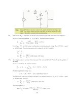
A single-phase power system is shown in Figure P2-1. The power source feeds a 100-kVA 14/2.4-kV
transformer through a feeder impedance of 40.0 + j150
Ω
. The transformer’s equivalent series impedance
referred to its low-voltage side is 0.12 + j0.5
Ω
. The load on the transformer is 90 kW at 0.80 PF lagging
and 2300 V.

(a) What is the voltage at the power source of the system?
(b) What is the voltage regulation of the transformer?
(c) How efficient is the overall power system?
S
OLUTION

To solve this problem, we will refer the circuit to the secondary (low-voltage) side. The feeder’s impedance

referred to the secondary side is

()
2
line
2.4 kV
40 150 1.18 4.41
14 kV
Zjj

′
=Ω+Ω=+Ω




29
The secondary current
S
I is given by

()()
90 kW
46.03 A
2300 V 0.85
S
I ==
46.03 31.8 A
S
=∠−°I

(a) The voltage at the power source of this system (referred to the secondary side) is

EQlinesource
ZZ
SSS
IIVV +
′
+=
′


()()()()
source
2300 0 V 46.03 31.8 A 1.18 4.11 46.03 31.8 A 0.12 0.5 jj
′
= ∠ ° + ∠− ° + Ω + ∠− ° + ΩV

source
2467 3.5 V
′
=∠°V

Therefore, the voltage at the power source is

()
source
14 kV
2467 3.5 V 14.4 3.5 kV
2.4 kV
=∠° =∠°

V

(b) To find the voltage regulation of the transformer, we must find the voltage at the primary side of the
transformer (referred to the secondary side) under full load conditions:

EQ
Z
SSP
IVV +=
′


()()
2300 0 V 46.03 31.8 A 0.12 0.5 2317 0.41 V
P
j
′
=∠°+ ∠−° +Ω=∠°V
There is a voltage drop of 17 V under these load conditions. Therefore the voltage regulation of the
transformer is

2317 2300
VR 100% 0.74%
2300
−
=×=

(c) The overall efficiency of the power system will be the ratio of the output power to the input power.
The output power supplied to the load is P
OUT

= 90 kW. The input power supplied by the source is

()( )
IN source
cos 2467 V 46.03 A cos 35.3 92.68 kW
S
PV I
θ
′
== °=
Therefore, the efficiency of the power system is

OUT
IN
90 kW
100% 100% 97.1%
92.68 kW
P
P
η
=× = × =
2-5. When travelers from the USA and Canada visit Europe, they encounter a different power distribution
system. Wall voltages in North America are 120 V rms at 60 Hz, while typical wall voltages in Europe are
220 to 240 V at 50 Hz. Many travelers carry small step-up / step-down transformers so that they can use
their appliances in the countries that they are visiting. A typical transformer might be rated at 1-kVA and
120/240 V. It has 500 turns of wire on the 120-V side and 1000 turns of wire on the 240-V side. The
magnetization curve for this transformer is shown in Figure P2-2, and can be found in file
p22_mag.dat

at this book’s Web site.

30

(a) Suppose that this transformer is connected to a 120-V, 60 Hz power source with no load connected
to the 240-V side. Sketch the magnetization current that would flow in the transformer. (Use
MATLAB to plot the current accurately, if it is available.) What is the rms amplitude of the
magnetization current? What percentage of full-load current is the magnetization current?
(b) Now suppose that this transformer is connected to a 240-V, 50 Hz power source with no load
connected to the 120-V side. Sketch the magnetization current that would flow in the transformer. (Use
MATLAB to plot the current accurately, if it is available.) What is the rms amplitude of the
magnetization current? What percentage of full-load current is the magnetization current?
(c) In which case is the magnetization current a higher percentage of full-load current? Why?
Note: An electronic version of this magnetization curve can be found in file
p22_mag.dat
, which can be used with MATLAB programs. Column 1
contains the MMF in A
⋅
turns, and column 2 contains the resulting flux in
webers.
S
OLUTION

(a) When this transformer is connected to a 120-V 60 Hz source, the flux in the core will be given by the
equation

cos )( t
N
V
t
P

M
ω
ω
φ
−= (2-101)
The magnetization current required for any given flux level can be found from Figure P2-2, or alternately
from the equivalent table in file
p22_mag.dat. The MATLAB program shown below calculates the flux
level at each time, the corresponding magnetization current, and the rms value of the magnetization current.

% M-file: prob2_5a.m
% M-file to calculate and plot the magnetization
% current of a 120/240 transformer operating at
% 120 volts and 60 Hz. This program also

31
% calculates the rms value of the mag. current.

% Load the magnetization curve. It is in two
% columns, with the first column being mmf and
% the second column being flux.
load p22_mag.dat;
mmf_data = p22(:,1);
flux_data = p22(:,2);

% Initialize values
S = 1000; % Apparent power (VA)
Vrms = 120; % Rms voltage (V)
VM = Vrms * sqrt(2); % Max voltage (V)
NP = 500; % Primary turns

% Calculate angular velocity for 60 Hz
freq = 60; % Freq (Hz)
w = 2 * pi * freq;

% Calculate flux versus time
time = 0:1/3000:1/30; % 0 to 1/30 sec
flux = -VM/(w*NP) * cos(w .* time);

% Calculate the mmf corresponding to a given flux
% using the MATLAB interpolation function.
mmf = interp1(flux_data,mmf_data,flux);

% Calculate the magnetization current
im = mmf / NP;

% Calculate the rms value of the current
irms = sqrt(sum(im.^2)/length(im));
disp(['The rms current at 120 V and 60 Hz is ', num2str(irms)]);

% Calculate the full-load current
i_fl = S / Vrms;

% Calculate the percentage of full-load current
percnt = irms / i_fl * 100;
disp(['The magnetization current is ' num2str(percnt)
'% of full-load current.']);

% Plot the magnetization current.
figure(1)

plot(time,im);
title ('\bfMagnetization Current at 120 V and 60 Hz');
xlabel ('\bfTime (s)');
ylabel ('\bf\itI_{m} \rm(A)');
axis([0 0.04 -0.5 0.5]);
grid on;
When this program is executed, the results are

» prob2_5a
The rms current at 120 V and 60 Hz is 0.31863
The magnetization current is 3.8236% of full-load current.

32
The rms magnetization current is 0.318 A. Since the full-load current is 1000 VA / 120 V = 8.33 A, the
magnetization current is 3.82% of the full-load current. The resulting plot is

(b) When this transformer is connected to a 240-V 50 Hz source, the flux in the core will be given by the
equation

cos )( t
N
V
t
S
M
ω
ω
φ
−=

The magnetization current required for any given flux level can be found from Figure P2-2, or alternately
from the equivalent table in file
p22_mag.dat
. The MATLAB program shown below calculates the flux
level at each time, the corresponding magnetization current, and the rms value of the magnetization current.

% M-file: prob2_5b.m
% M-file to calculate and plot the magnetization
% current of a 120/240 transformer operating at
% 240 volts and 50 Hz. This program also
% calculates the rms value of the mag. current.

% Load the magnetization curve. It is in two
% columns, with the first column being mmf and
% the second column being flux.
load p22_mag.dat;
mmf_data = p22(:,1);
flux_data = p22(:,2);

% Initialize values
S = 1000; % Apparent power (VA)
Vrms = 240; % Rms voltage (V)
VM = Vrms * sqrt(2); % Max voltage (V)
NP = 1000; % Primary turns

% Calculate angular velocity for 50 Hz
freq = 50; % Freq (Hz)
w = 2 * pi * freq;

% Calculate flux versus time

time = 0:1/2500:1/25; % 0 to 1/25 sec

33
flux = -VM/(w*NP) * cos(w .* time);

% Calculate the mmf corresponding to a given flux
% using the MATLAB interpolation function.
mmf = interp1(flux_data,mmf_data,flux);

% Calculate the magnetization current
im = mmf / NP;

% Calculate the rms value of the current
irms = sqrt(sum(im.^2)/length(im));
disp(['The rms current at 50 Hz is ', num2str(irms)]);

% Calculate the full-load current
i_fl = S / Vrms;

% Calculate the percentage of full-load current
percnt = irms / i_fl * 100;
disp(['The magnetization current is ' num2str(percnt)
'% of full-load current.']);

% Plot the magnetization current.
figure(1);
plot(time,im);
title ('\bfMagnetization Current at 240 V and 50 Hz');
xlabel ('\bfTime (s)');
ylabel ('\bf\itI_{m} \rm(A)');

axis([0 0.04 -0.5 0.5]);
grid on;
When this program is executed, the results are

» prob2_5b
The rms current at 50 Hz is 0.22973
The magnetization current is 5.5134% of full-load current.
The rms magnetization current is 0.318 A. Since the full-load current is 1000 VA / 240 V = 4.17 A, the
magnetization current is 5.51% of the full-load current. The resulting plot is


34
(c) The magnetization current is a higher percentage of the full-load current for the 50 Hz case than for
the 60 Hz case. This is true because the peak flux is higher for the 50 Hz waveform, driving the core
further into saturation.
2-6. A 15-kVA 8000/230-V distribution transformer has an impedance referred to the primary of 80 + j300
Ω
.
The components of the excitation branch referred to the primary side are
Ω= k 350
C
R
and
Ω= k 70
M
X .
(a) If the primary voltage is 7967 V and the load impedance is Z
L
= 3.2 + j1.5
Ω

, what is the secondary
voltage of the transformer? What is the voltage regulation of the transformer?
(b) If the load is disconnected and a capacitor of –j3.5
Ω
is connected in its place, what is the secondary
voltage of the transformer? What is its voltage regulation under these conditions?
S
OLUTION

(a) The easiest way to solve this problem is to refer all components to the primary side of the
transformer. The turns ratio is a = 8000/230 = 34.78. Thus the load impedance referred to the primary
side is

()( )
2
34.78 3.2 1.5 3871 1815
L
Zjj
′
=+Ω=+Ω

The referred secondary current is

()( )
7967 0 V 7967 0 V
1.78 28.2 A
80 300 3871 1815 4481 28.2
S
jj
∠° ∠°

′
===∠−°
+Ω+ + Ω ∠°Ω
I
and the referred secondary voltage is

()()
1.78 28.2 A 3871 1815 7610 3.1 V
SSL
Zj
′′′
= = ∠− ° + Ω = ∠− °VI

The actual secondary voltage is thus

7610 3.1 V
218.8 3.1 V
34.78
S
S
a
′
∠− °
== = ∠−°
V
V

The voltage regulation is

7967-7610

VR 100% 4.7%
7610
=×=

(b) The easiest way to solve this problem is to refer all components to the primary side of the
transformer. The turns ratio is again a = 34.78. Thus the load impedance referred to the primary side is

()( )
2
34.78 3.5 4234
L
Zjj
′
=−Ω=−Ω
The referred secondary current is

()()
7967 0 V 7967 0 V
2.025 88.8 A
80 300 4234 3935 88.8
S
jj
∠° ∠°
′
===∠°
+Ω+− Ω ∠−°Ω
I
and the referred secondary voltage is

()()

2.25 88.8 A 4234 8573 1.2 V
SSL
Zj
′′′
==∠°−Ω=∠−°VI

The actual secondary voltage is thus

35

8573 1.2 V
246.5 1.2 V
34.78
S
S
a
′
∠− °
== = ∠−°
V
V

The voltage regulation is

7967 8573
VR 100% 7.07%
8573
−
=×=−

2-7. A 5000-kVA 230/13.8-kV single-phase power transformer has a per-unit resistance of 1 percent and a per-
unit reactance of 5 percent (data taken from the transformer’s nameplate). The open-circuit test performed
on the low-voltage side of the transformer yielded the following data:

V
OC
kV= 138. A 1.15
OC
=I kW 9.44
OC
=P
(a) Find the equivalent circuit referred to the low-voltage side of this transformer.
(b) If the voltage on the secondary side is 13.8 kV and the power supplied is 4000 kW at 0.8 PF
lagging, find the voltage regulation of the transformer. Find its efficiency.
S
OLUTION

(a) The open-circuit test was performed on the low-voltage side of the transformer, so it can be used to
directly find the components of the excitation branch relative to the low-voltage side.

EX
15.1 A
0.0010942
13.8 kV
CM
YGjB=− = =


()()
11

OC
OC OC
44.9 kW
cos cos 77.56
13.8 kV 15.1 A
P
VI
θ
−−
== =°

EX
0.0010942 77.56 S 0.0002358 0.0010685 S
CM
YGjB j=− = ∠− °= −


1
4240
C
C
R
G
== Ω

1
936
M
M
X

B
==Ω
The base impedance of this transformer referred to the secondary side is

()
2
2
base
base
base
13.8 kV
38.09
5000 kVA
V
Z
S
== = Ω

so
(
)
(
)
EQ
0.01 38.09 0.38 R =Ω=Ω and
(
)
(
)
EQ

0.05 38.09 1.9 X =Ω=Ω. The resulting equivalent circuit
is shown below:


36

Ω= 38.0
sEQ,
R Ω= 9.1
sEQ,
jX

Ω= 4240
,sC
R

Ω= 936
,sM
X


(b) If the load on the secondary side of the transformer is 4000 kW at 0.8 PF lagging and the secondary
voltage is 13.8 kV, the secondary current is

()()
LOAD
4000 kW
362.3 A
PF 13.8 kV 0.8
S

S
P
I
V
== =
362.3 36.87 A
S
=∠−°I
The voltage on the primary side of the transformer (referred to the secondary side) is

EQPSS
Z
′
=+
VVI

()()
13,800 0 V 362.3 36.87 A 0.38 1.9 14,330 1.9 V
P
j
′
=∠°+∠−° +Ω=∠°V

There is a voltage drop of 14 V under these load conditions. Therefore the voltage regulation of the
transformer is

14,330 13,800
VR 100% 3.84%
13,800
−

=×=

The transformer copper losses and core losses are

()()
2
2
CU EQ,
362.3 A 0.38 49.9 kW
SS
PIR== Ω=


(
)
()
2
2
core
14,330 V
48.4 kW
4240
P
C
V
P
R
′
== =
Ω

Therefore the efficiency of this transformer at these conditions is

OUT
OUT CU core
4000 kW
100% 97.6%
4000 kW 49.9 kW 48.4 kW
P
PPP
η
=×= =
++ + +

2-8. A 200-MVA 15/200-kV single-phase power transformer has a per-unit resistance of 1.2 percent and a per-
unit reactance of 5 percent (data taken from the transformer’s nameplate). The magnetizing impedance is
j80 per unit.
(a) Find the equivalent circuit referred to the low-voltage side of this transformer.
(b) Calculate the voltage regulation of this transformer for a full-load current at power factor of 0.8
lagging.
(c) Assume that the primary voltage of this transformer is a constant 15 kV, and plot the secondary voltage
as a function of load current for currents from no-load to full-load. Repeat this process for power
factors of 0.8 lagging, 1.0, and 0.8 leading.
S
OLUTION


(a) The base impedance of this transformer referred to the primary (low-voltage) side is

()

2
2
base
base
base
15 kV
1.125
200 MVA
V
Z
S
== =Ω
so
(
)
(
)
EQ
0.012 1.125 0.0135 R =Ω=Ω


()( )
EQ
0.05 1.125 0.0563 X =Ω=Ω

37

()( )
100 1.125 112.5
M

X =Ω=Ω
The equivalent circuit is


EQ,
0.0135
P
R =Ω
EQ,
0.0563
P
Xj=Ω
not specified
C
R = 112.5
M
X =Ω

(b) If the load on the secondary side of the transformer is 200 MVA at 0.8 PF lagging, and the referred
secondary voltage is 15 kV, then the referred secondary current is

()()
LOAD
200 MVA
16,667 A
PF 15 kV 0.8
S
S
P
I

V
′
== =

16,667 36.87 A
S
′
=∠−°
I
The voltage on the primary side of the transformer is

EQ,PSSP
Z
′′
=+
VV I


()()
15,000 0 V 16,667 36.87 A 0.0135 0.0563 15, 755 2.24 V
P
j=∠°+ ∠−° + Ω=∠°V
Therefore the voltage regulation of the transformer is

15,755-15,000
VR 100% 5.03%
15,000
=×=

(c) This problem is repetitive in nature, and is ideally suited for MATLAB. A program to calculate the
secondary voltage of the transformer as a function of load is shown below:

% M-file: prob2_8.m
% M-file to calculate and plot the secondary voltage
% of a transformer as a function of load for power
% factors of 0.8 lagging, 1.0, and 0.8 leading.
% These calculations are done using an equivalent
% circuit referred to the primary side.

% Define values for this transformer
VP = 15000; % Primary voltage (V)
amps = 0:166.67:16667; % Current values (A)
Req = 0.0135; % Equivalent R (ohms)
Xeq = 0.0563; % Equivalent X (ohms)

% Calculate the current values for the three
% power factors. The first row of I contains
% the lagging currents, the second row contains
% the unity currents, and the third row contains

38
% the leading currents.
I(1,:) = amps .* ( 0.8 - j*0.6); % Lagging
I(2,:) = amps .* ( 1.0 ); % Unity
I(3,:) = amps .* ( 0.8 + j*0.6); % Leading

% Calculate VS referred to the primary side
% for each current and power factor.
aVS = VP - (Req.*I + j.*Xeq.*I);

% Refer the secondary voltages back to the
% secondary side using the turns ratio.
VS = aVS * (200/15);

% Plot the secondary voltage (in kV!) versus load
plot(amps,abs(VS(1,:)/1000),'b-','LineWidth',2.0);
hold on;
plot(amps,abs(VS(2,:)/1000),'k ','LineWidth',2.0);
plot(amps,abs(VS(3,:)/1000),'r ','LineWidth',2.0);
title ('\bfSecondary Voltage Versus Load');
xlabel ('\bfLoad (A)');
ylabel ('\bfSecondary Voltage (kV)');
legend('0.8 PF lagging','1.0 PF','0.8 PF leading');
grid on;
hold off;
The resulting plot of secondary voltage versus load is shown below:

2-9. A three-phase transformer bank is to handle 600 kVA and have a 34.5/13.8-kV voltage ratio. Find the
rating of each individual transformer in the bank (high voltage, low voltage, turns ratio, and apparent
power) if the transformer bank is connected to
(a) Y-Y, (b) Y-∆, (c) ∆-Y, (d) ∆-∆, (e) open-∆, (f) open-
Y—open-
∆
.
S
OLUTION
For the first four connections, the apparent power rating of each transformer is 1/3 of the total
apparent power rating of the three-phase transformer. For the open-∆ and open-Y—open-∆ connections,
the apparent power rating is a bit more complicated. The 600 kVA must be 86.6% of the total apparent