Electric Machinery Fundamentals Power & Energy_5 docx

83

Figure (b)
(3) If SCR
1
and SCR
4
are now triggered again, the voltages across capacitors C
1
and C
2
will force
SCR
2
and SCR
3
to turn OFF. The cycle continues in this fashion.

Capacitors C
1
and C
2
are called commutating capacitors. Their purpose is to force one set of SCRs to turn
OFF when the other set turns ON.

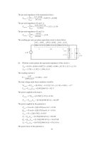
The output frequency of this rectifier-inverter circuit is controlled by the rates at which the SCRs are
triggered. The resulting voltage and current waveforms (assuming a resistive load) are shown below.

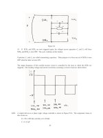
3-13. A simple full-wave ac phase angle voltage controller is shown in Figure P3-8. The component values in
this circuit are:

R = 20 to 300 k
Ω
, currently set to 80 k
Ω

C = 0.15
µ
F

84

BO
V = 40 V (for PNPN Diode D
1
)

BO
V = 250 V (for SCR
1
)
( ) sin volts
sM
vt V t
ω
=
where
M
V = 169.7 V and
ω
= 377 rad/s

(a) At what phase angle do the PNPN diode and the SCR turn on?
(b) What is the rms voltage supplied to the load under these circumstances?


Note: Problem 3-13 is significantly harder for many students, since it involves
solving a differential equation with a forcing function. This problem should
only be assigned if the class has the mathematical sophistication to handle it.
S
OLUTION
At the beginning of each half cycle, the voltages across the PNPN diode and the SCR will both be
smaller then their respective breakover voltages, so no current will flow to the load (except for the very tiny
current charging capacitor C), and v
load
(t) will be 0 volts. However, capacitor C charges up through
resistor R, and when the voltage v
C
(t) builds up to the breakover voltage of D
1
, the PNPN diode will start to
conduct. This current flows through the gate of SCR
1
, turning the SCR ON. When it turns ON, the
voltage across the SCR will drop to 0, and the full source voltage v
S
(t) will be applied to the load,
producing a current flow through the load. The SCR continues to conduct until the current through it falls
below I
H
, which happens at the very end of the half cycle.
Note that after D

1
turns on, capacitor C discharges through it and the gate of the SCR. At the end of the
half cycle, the voltage on the capacitor is again essentially 0 volts, and the whole process is ready to start
over again at the beginning of the next half cycle.
To determine when the PNPN diode and the SCR fire in this circuit, we must determine when v
C
(t) exceeds
V
BO
for D
1
. This calculation is much harder than in the examples in the book, because in the previous
problems the source was a simple DC voltage source, while here the voltage source is sinusoidal. However,
the principles are identical.
(a) To determine when the SCR will turn ON, we must calculate the voltage v
C
(t), and then solve for the time
at which v
C
(t) exceeds V
BO
for D
1
. At the beginning of the half cycle, D
1
and SCR
1
are OFF, and the
voltage across the load is essentially 0, so the entire source voltage v
S

(t) is applied to the series RC circuit.
To determine the voltage v
C
(t) on the capacitor, we can write a Kirchhoff's Current Law equation at the
node above the capacitor and solve the resulting equation for v
C
(t).

12
0ii+= (since the PNPN diode is an open circuit at this time)

85

1
0
C
C
vv d
Cv
Rdt
−
+=


1
11
CC
d
vv v
dt RC RC

+=


1
sin
M
CC
dV
vv t
dt RC RC
ω
+=

The solution can be divided into two parts, a natural response and a forced response. The natural response
is the solution to the equation

1
0
CC
d
vv
dt RC
+=

The solution to the natural response equation is

()

,
e

t
RC
Cn
vtA
−
=
where the constant A must be determined from the initial conditions in the system. The forced response is
the steady-state solution to the equation

1
sin
M
CC
dV
vv t
dt RC RC
ω
+=

It must have a form similar to the forcing function, so the solution will be of the form

(
)
,1 2
sin cos
Cf
vtB tB t
ωω
=+

where the constants
1
B
and
2
B
must be determined by substitution into the original equation. Solving for
1
B
and
2
B
yields:

()()
12 12
1
sin cos sin cos sin
M
dV
BtBtBtBt t
dt RC RC
ωω ωω ω
++ +=


()()
12 12
1
cos in sin cos sin

M
V
BtBst B tB t t
RC RC
ωωω ω ω ω ω
−+ +=


cosine equation:

12
1
0BB
RC
ω
+=
⇒

21
BRCB
ω
=−

sine equation:

21
1
M
V
BB

RC RC
ω
−+ =


2
11
1

M
V
RC B B
RC RC
ω
+=


2
1
1

M
V
RC B
RC RC
ω

+=

222
1
1
M
RC V
B
RC RC
ω

+
=



Finally,

86

1
222
1
M
V
B
RC
ω
=
+

and
2
222
1
M
RC V
B
RC
ω
ω
−
=
+

Therefore, the forced solution to the equation is

()
,
222 222

sin cos
11
MM
Cf
VRCV
vt t t
RC RC
ω
ωω
ωω

=−
++

and the total solution is

(
)
(
)
(
)
,,CCnCf
vt v t v t=+

()

222 222

sin cos
11
t
MM
RC
C
VRCV
vt Ae t t
RC RC
ω
ωω
ωω

−
=+ −
++

The initial condition for this problem is that the voltage on the capacitor is zero at the beginning of the half-
cycle:

()
0

222 222

0 sin 0 cos 00
11
MM
RC
C
VRCV
vAe
RC RC
ω
ωω
−
=+ − =
++


222

0

1
M
RC V
A
RC
ω
ω
−=
+


222

1
M
RC V
A
RC
ω
ω
=
+

Therefore, the voltage across the capacitor as a function of time before the PNPN diode fires is

()

222 222 222

sin cos

11 1
t
MM M
RC
C
RC V V RC V
vt e t t
RC RC RC
ωω
ωω
ωω ω
−
=+ −
++ +

If we substitute the known values for R, C, ω, and V
M
, this equation becomes

(
)
83.3
35.76 7.91 sin 35.76 cos
t
C
vt e t t
ωω
−
=+−
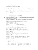
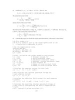
This equation is plotted below:

87

It reaches a voltage of 40 V at a time of 4.8 ms. Since the frequency of the waveform is 60 Hz, the
waveform there are 360
°
in 1/60 s, and the firing angle
α
is

()
360
4.8 ms 103.7
1/ 60 s
α
°

==°


or 1.810 radians

Note: This problem could also have been solved using Laplace Transforms, if desired.
(b) The rms voltage applied to the load is

/
222
rms
1
() sin

M
VvtdtVtdt
T
πω
α
ω
ω
π
==



/
2
rms
11
sin 2
24
M
V
Vtt
πω
α
ωω
π

=−

()()






−−−=
απαπ
π
2sin2sin
4
1
2
1
2
rms
M
V
V

Since
α
= 1.180 radians, the rms voltage is

rms
0.1753 0.419 71.0 V
MM
VV V===

3-14. Figure P3-9 shows a three-phase full-wave rectifier circuit supplying power to a dc load. The circuit uses
SCRs instead of diodes as the rectifying elements.
(a) What will the load voltage and ripple be if each SCR is triggered as soon as it becomes forward biased?
At what phase angle should the SCRs be triggered in order to operate this way? Sketch or plot the
output voltage for this case.
(b) What will the rms load voltage and ripple be if each SCR is triggered at a phase angle of 90° (that is,
half way through the half-cycle in which it is forward biased)? Sketch or plot the output voltage for
this case.

88

S
OLUTION
Assume that the three voltages applied to this circuit are:

(
)
sin
AM
vt V t
ω
=

(
)
(
)
sin 2 / 3
BM
vt V t

ωπ
=−


(
)
(
)
sin 2 / 3
CM
vt V t
ωπ
=+
The period of the input waveforms is T, where
2/T
πω
=
. For the purpose of the calculations in this
problem, we will assume that
ω
is 377 rad/s (60 Hz).
(a) The when the SCRs start to conduct as soon as they are forward biased, this circuit is just a three-
phase full-wave bridge, and the output voltage is identical to that in Problem 3-2. The sketch of output
voltage is reproduced below, and the ripple is 4.2%. The following table shows which SCRs must conduct
in what order to create the output voltage shown below. The times are expressed as multiples of the period
T of the input waveforms, and the firing angle is in degrees relative to time zero.

Start Time
(
ω

t
)
Stop Time
(
ω
t
)
Positive
Phase
Negative
Phase
Conducting
SCR
(Positive)
Conducting
SCR
(Negative)
Triggered
SCR
Firing
Angle
12/T−

12/T

c b SCR
3
SCR
5
SCR

5

-30
°

12/T 12/3T
a b SCR
1
SCR
5
SCR
1

30°
12/3T

12/5T

a c SCR
1
SCR
6
SCR
6

90
°

12/5T

12/7T

b c SCR
2
SCR
6
SCR
2

150°
12/7T

12/9T

b a SCR
2
SCR
4
SCR
4

210
°

12/9T

12/11T

c a SCR
3

SCR
4
SCR
3

270
°

12/11T 12/T
c b SCR
3
SCR
5
SCR
5

330°


89
T
/12

(b) If each SCR is triggered halfway through the half-cycle during which it is forward biased, the
resulting phase a, b, and c voltages will be zero before the first half of each half-cycle, and the full
sinusoidal value for the second half of each half-cycle. These waveforms are shown below. (These plots
were created by the MATLAB program that appears later in this answer.)

and the resulting output voltage will be:

90

A MATLAB program to generate these waveforms and to calculate the ripple on the output waveform is
shown below. The first function
biphase_controller.m
generates a switched ac waveform. The
inputs to this function are the current phase angle in degrees, the offset angle of the waveform in degrees,
and the firing angle in degrees.

function volts = biphase_controller(wt,theta0,fire)
% Function to simulate the output of an ac phase
% angle controller that operates symmetrically on
% positive and negative half cycles. Assume a peak
% voltage VM = 120 * SQRT(2) = 170 V for convenience.
%
% wt = Current phase in degrees
% theta0 = Starting phase angle in degrees
% fire = Firing angle in degrees

% Degrees to radians conversion factor
deg2rad = pi / 180;

% Remove phase ambiguities: 0 <= wt < 360 deg
ang = wt + theta0;
while ang >= 360
ang = ang - 360;
end
while ang < 0
ang = ang + 360;
end

% Simulate the output of the phase angle controller.
if (ang >= fire & ang <= 180)
volts = 170 * sin(ang * deg2rad);
elseif (ang >= (fire+180) & ang <= 360)
volts = 170 * sin(ang * deg2rad);
else

91
volts = 0;
end

The main program below creates and plots the three-phase waveforms, calculates and plots the output
waveform, and determines the ripple in the output waveform.

% M-file: prob3_14b.m
% M-file to calculate and plot the three phase voltages
% when each SCR in a three-phase full-wave rectifier
% triggers at a phase angle of 90 degrees.

% Calculate the waveforms for times from 0 to 1/30 s
t = (0:1/21600:1/30);
deg = zeros(size(t));
rms = zeros(size(t));
va = zeros(size(t));
vb = zeros(size(t));
vc = zeros(size(t));
out = zeros(size(t));
for ii = 1:length(t)

% Get equivalent angle in degrees. Note that
% 1/60 s = 360 degrees for a 60 Hz waveform!
theta = 21600 * t(ii);

% Calculate the voltage in each phase at each
% angle.
va(ii) = biphase_controller(theta,0,90);
vb(ii) = biphase_controller(theta,-120,90);
vc(ii) = biphase_controller(theta,120,90);

end

% Calculate the output voltage of the rectifier
for ii = 1:length(t)
vals = [ va(ii) vb(ii) vc(ii) ];
out(ii) = max( vals ) - min( vals );
end

% Calculate and display the ripple
disp( ['The ripple is ' num2str(ripple(out))] );

% Plot the voltages versus time
figure(1)
plot(t,va,'b','Linewidth',2.0);
hold on;
plot(t,vb,'r:','Linewidth',2.0);
plot(t,vc,'k ','Linewidth',2.0);
title('\bfPhase Voltages');
xlabel('\bfTime (s)');
ylabel('\bfVoltage (V)');

grid on;
legend('Phase a','Phase b','Phase c');
hold off;


92
% Plot the output voltages versus time
figure(2)
plot(t,out,'b','Linewidth',2.0);
title('\bfOutput Voltage');
xlabel('\bfTime (s)');
ylabel('\bfVoltage (V)');
axis( [0 1/30 0 260]);
grid on;
hold off;
When this program is executed, the results are:

»
prob_3_14b

The ripple is 30.9547
3-15. Write a MATLAB program that imitates the operation of the Pulse-Width Modulation circuit shown in
Figure 3-55, and answer the following questions.
(a) Assume that the comparison voltages
vt
x
()
and
vt
y

()
have peak amplitudes of 10 V and a frequency
of 500 Hz. Plot the output voltage when the input voltage is
vt ft
in
() sin=10 2π V, and f = 50 Hz.
(b) What does the spectrum of the output voltage look like? What could be done to reduce the harmonic
content of the output voltage?
(c) Now assume that the frequency of the comparison voltages is increased to 1000 Hz. Plot the output
voltage when the input voltage is
vt ft
in
() sin=10 2π V, and f = 50 Hz.
(d) What does the spectrum of the output voltage in (c) look like?
(e) What is the advantage of using a higher comparison frequency and more rapid switching in a PWM
modulator?
S
OLUTION
The PWM circuit is shown below:


93

(a) To write a MATLAB simulator of this circuit, note that if
in
v >
x
v , then
u
v =

DC
V , and if
in
v <
x
v ,
then
u
v
= 0. Similarly, if
in
v
>
y
v
, then
v
v
= 0, and if
in
v
<
y
v
, then
v
v
=
DC
V

. The output voltage is
then
uv
vvv −=
out
. A MATLAB function that performs these calculations is shown below. (Note that
this function arbitrarily assumes that
DC
V = 100 V. It would be easy to modify the function to use any
arbitrary dc voltage, if desired.)

function [vout,vu,vv] = vout(vin, vx, vy)
% Function to calculate the output voltage of a
% PWM modulator from the values of vin and the
% reference voltages vx and vy. This function
% arbitrarily assumes that VDC = 100 V.
%
% vin = Input voltage
% vx = x reference
% vy = y reference
% vout = Ouput voltage
% vu, vv = Components of output voltage

94
% fire = Firing angle in degrees

% vu
if ( vin > vx )
vu = 100;
else

vu = 0;
end

% vv
if ( vin >= vy )
vv = 0;
else
vv = 100;
end

% Caclulate vout
vout = vv - vu;

Now we need a MATLAB program to generate the input voltage
()
tv
in
and the reference voltages
()
tv
x

and
()
tv
y
. After the voltages are generated, function vout will be used to calculate
()
tv
out

and the
frequency spectrum of
()
tv
out
. Finally, the program will plot
()
tv
in
,
()
tv
x
and
()
tv
y
,
()
tv
out
, and the
spectrum of
()
tv
out
. (Note that in order to have a valid spectrum, we need to create several cycles of the
60 Hz output waveform, and we need to sample the data at a fairly high frequency. This problem creates 4
cycles of
()

tv
out
and samples all data at a 20,000 Hz rate.)

% M-file: prob3_15a.m
% M-file to calculate the output voltage from a PWM
% modulator with a 500 Hz reference frequency. Note
% that the only change between this program and that
% of part b is the frequency of the reference "fr".

%
Sample the data at 20000 Hz
to get enough information
% for spectral analysis. Declare arrays.
fs = 20000; % Sampling frequency (Hz)
t = (0:1/fs:4/15); % Time in seconds
vx = zeros(size(t)); % vx
vy = zeros(size(t)); % vy
vin = zeros(size(t)); % Driving signal
vu = zeros(size(t)); % vx
vv = zeros(size(t)); % vy
vout = zeros(size(t)); % Output signal
fr = 500; % Frequency of reference signal
T = 1/fr; % Period of refernce signal

% Calculate vx at fr = 500 Hz.
for ii = 1:length(t)
vx(ii) = vref(t(ii),T);
vy(ii) = - vx(ii);
end

% Calculate vin as a 50 Hz sine wave with a peak voltage of

95
% 10 V.
for ii = 1:length(t)
vin(ii) = 10 * sin(2*pi*50*t(ii));
end

% Now calculate vout
for ii = 1:length(t)
[vout(ii) vu(ii) vv(ii)] = vout(vin(ii), vx(ii), vy(ii));
end

% Plot the reference voltages vs time
figure(1)
plot(t,vx,'b','Linewidth',1.0);
hold on;
plot(t,vy,'k ','Linewidth',1.0);
title('\bfReference Voltages for fr = 500 Hz');
xlabel('\bfTime (s)');
ylabel('\bfVoltage (V)');
legend('vx','vy');
axis( [0 1/30 -10 10]);
hold off;

% Plot the input voltage vs time
figure(2)
plot(t,vin,'b','Linewidth',1.0);
title('\bfInput Voltage');

xlabel('\bfTime (s)');
ylabel('\bfVoltage (V)');
axis( [0 1/30 -10 10]);

% Plot the output voltages versus time
figure(3)
plot(t,vout,'b','Linewidth',1.0);
title('\bfOutput Voltage for fr = 500 Hz');
xlabel('\bfTime (s)');
ylabel('\bfVoltage (V)');
axis( [0 1/30 -120 120]);

% Now calculate the spectrum of the output voltage
spec = fft(vout);

% Calculate sampling frequency labels
len = length(t);
df = fs / len;
fstep = zeros(size(t));
for ii = 2:len/2
fstep(ii) = df * (ii-1);
fstep(len-ii+2) = -fstep(ii);
end

% Plot the spectrum
figure(4);
plot(fftshift(fstep),fftshift(abs(spec)));
title('\bfSpectrum of Output Voltage for fr = 500 Hz');
xlabel('\bfFrequency (Hz)');
ylabel('\bfAmplitude');

96

% Plot a closeup of the near spectrum
% (positive side only)
figure(5);
plot(fftshift(fstep),fftshift(abs(spec)));
title('\bfSpectrum of Output Voltage for fr = 500 Hz');
xlabel('\bfFrequency (Hz)');
ylabel('\bfAmplitude');
set(gca,'Xlim',[0 1000]);
When this program is executed, the input, reference, and output voltages are:



97

(b) The output spectrum of this PWM modulator is shown below. There are two plots here, one showing
the entire spectrum, and the other one showing the close-in frequencies (those under 1000 Hz), which will
have the most effect on machinery. Note that there is a sharp peak at 50 Hz, which is there desired
frequency, but there are also strong contaminating signals at about 850 Hz and 950 Hz. If necessary, these
components could be filtered out using a low-pass filter.


98

(c) A version of the program with 1000 Hz reference functions is shown below:

% M-file: prob3_15b.m
% M-file to calculate the output voltage from a PWM

% modulator with a 1000 Hz reference frequency. Note
% that the only change between this program and that
% of part a is the frequency of the reference "fr".

% Sample the data at 20000 Hz to get enough information
% for spectral analysis. Declare arrays.
fs = 20000; % Sampling frequency (Hz)
t = (0:1/fs:4/15); % Time in seconds
vx = zeros(size(t)); % vx
vy = zeros(size(t)); % vy
vin = zeros(size(t)); % Driving signal
vu = zeros(size(t)); % vx
vv = zeros(size(t)); % vy
vout = zeros(size(t)); % Output signal
fr = 1000; % Frequency of reference signal
T = 1/fr; % Period of refernce signal

% Calculate vx at 1000 Hz.
for ii = 1:length(t)
vx(ii) = vref(t(ii),T);
vy(ii) = - vx(ii);
end

% Calculate vin as a 50 Hz sine wave with a peak voltage of
% 10 V.
for ii = 1:length(t)
vin(ii) = 10 * sin(2*pi*50*t(ii));
end

99
% Now calculate vout
for ii = 1:length(t)
[vout(ii) vu(ii) vv(ii)] = vout(vin(ii), vx(ii), vy(ii));
end

% Plot the reference voltages vs time
figure(1)
plot(t,vx,'b','Linewidth',1.0);
hold on;
plot(t,vy,'k ','Linewidth',1.0);
title('\bfReference Voltages for fr = 1000 Hz');
xlabel('\bfTime (s)');
ylabel('\bfVoltage (V)');
legend('vx','vy');
axis( [0 1/30 -10 10]);
hold off;

% Plot the input voltage vs time
figure(2)
plot(t,vin,'b','Linewidth',1.0);
title('\bfInput Voltage');
xlabel('\bfTime (s)');
ylabel('\bfVoltage (V)');
axis( [0 1/30 -10 10]);

% Plot the output voltages versus time
figure(3)
plot(t,vout,'b','Linewidth',1.0);
title('\bfOutput Voltage for fr = 1000 Hz');

xlabel('\bfTime (s)');
ylabel('\bfVoltage (V)');
axis( [0 1/30 -120 120]);

% Now calculate the spectrum of the output voltage
spec = fft(vout);

% Calculate sampling frequency labels
len = length(t);
df = fs / len;
fstep = zeros(size(t));
for ii = 2:len/2
fstep(ii) = df * (ii-1);
fstep(len-ii+2) = -fstep(ii);
end

% Plot the spectrum
figure(4);
plot(fftshift(fstep),fftshift(abs(spec)));
title('\bfSpectrum of Output Voltage for fr = 1000 Hz');
xlabel('\bfFrequency (Hz)');
ylabel('\bfAmplitude');

% Plot a closeup of the near spectrum
% (positive side only)
figure(5);
plot(fftshift(fstep),fftshift(abs(spec)));

100
title('\bfSpectrum of Output Voltage for fr = 1000 Hz');

xlabel('\bfFrequency (Hz)');
ylabel('\bfAmplitude');
set(gca,'Xlim',[0 1000]);
When this program is executed, the input, reference, and output voltages are:



101

(d) The output spectrum of this PWM modulator is shown below.


102

(e) Comparing the spectra in (b) and (d), we can see that the frequencies of the first large sidelobes
doubled from about 900 Hz to about 1800 Hz when the reference frequency was doubled. This increase in
sidelobe frequency has two major advantages: it makes the harmonics easier to filter, and it also makes it
less necessary to filter them at all. Since large machines have their own internal inductances, they form
natural low-pass filters. If the contaminating sidelobes are at high enough frequencies, they will never
affect the operation of the machine. Thus, it is a good idea to design PWM modulators with a high
frequency reference signal and rapid switching.


103
Chapter 4:
AC Machinery Fundamentals
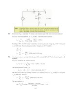
4-1. The simple loop is rotating in a uniform magnetic field shown in Figure 4-1 has the following
characteristics:

B = 05. T to the right

r
= 01.m

l = 05. m
ω
= 103 rad/s
(a) Calculate the voltage
et
tot
()induced in this rotating loop.
(b) Suppose that a 5
Ω
resistor is connected as a load across the terminals of the loop. Calculate the
current that would flow through the resistor.
(c) Calculate the magnitude and direction of the induced torque on the loop for the conditions in (b).
(d) Calculate the electric power being generated by the loop for the conditions in (b).
(e) Calculate the mechanical power being consumed by the loop for the conditions in (b). How does
this number compare to the amount of electric power being generated by the loop?
ω
m
r
v
ab
v
cd
B
N
S
B

is a uniform magnetic
field, aligned as shown.
a
b
c
d

S
OLUTION

(a) The induced voltage on a simple rotating loop is given by

(
)
ind
2 sin et rBl t
ω
=ω
(4-8)

() ( )( )( )( )
ind
2 0.1 m 103 rad/s 0.5 T 0.5 m sin103et t=

()
ind
5.15 sin103 Vet t=

(b) If a 5
Ω

resistor is connected as a load across the terminals of the loop, the current flow would be:

()
ind
5.15 sin 103 V
1.03 sin 103 A
5
et
it t
R
== =
Ω

(c) The induced torque would be:

()
ind
2 sin trilΒ
τθ
= (4-17)

() ( )( )( )( )
ind
2 0.1 m 1.03 sin A 0.5 m 0.5 T sin tt t
τωω
=


()
2

ind
0.0515 sin N m, counterclockwisett
τω
=⋅
(d) The instantaneous power generated by the loop is:

104

() ( )( )
2
ind
5.15 sin V 1.03 sin A 5.30 sin WPt e i t t t
ωω ω
== =
The average power generated by the loop is

2
ave
1
5.30 sin 2.65 W
T
Ptdt
T
ω
==


(e) The mechanical power being consumed by the loop is:

()

()
22
ind
0.0515 sin V 103 rad/s 5.30 sin WPt t
τω ω ω
== =

Note that the amount of mechanical power consumed by the loop is equal to the amount of electrical power
created by the loop. This machine is acting as a generator, converting mechanical power into electrical
power.
4-2. Develop a table showing the speed of magnetic field rotation in ac machines of 2, 4, 6, 8, 10, 12, and 14
poles operating at frequencies of 50, 60, and 400 Hz.
S
OLUTION
The equation relating the speed of magnetic field rotation to the number of poles and electrical
frequency is

120
e
m
f
n
P
=

The resulting table is
Number of Poles
e
f = 50 Hz
e

f = 60 Hz
e
f = 400 Hz
2 3000 r/min 3600 r/min 24000 r/min
4 1500 r/min 1800 r/min 12000 r/min
6 1000 r/min 1200 r/min 8000 r/min
8 750 r/min 900 r/min 6000 r/min
10 600 r/min 720 r/min 4800 r/min
12 500 r/min 600 r/min 4000 r/min
14 428.6 r/min 514.3 r/min 3429 r/min
4-3. A three-phase four-pole winding is installed in 12 slots on a stator. There are 40 turns of wire in each slot
of the windings. All coils in each phase are connected in series, and the three phases are connected in
∆
.
The flux per pole in the machine is 0.060 Wb, and the speed of rotation of the magnetic field is 1800 r/min.
(a) What is the frequency of the voltage produced in this winding?
(b) What are the resulting phase and terminal voltages of this stator?
S
OLUTION

(a) The frequency of the voltage produced in this winding is

()()
1800 r/min 4 poles
60 Hz
120 120
m
e
nP
f == =

(b) There are 12 slots on this stator, with 40 turns of wire per slot. Since this is a four-pole machine,
there are two sets of coils (4 slots) associated with each phase. The voltage in the coils in one pair of slots
is

()( )( )
2 2 40 t 0.060 Wb 60 Hz 640 V
AC
ENf
πφ π
== =
There are two sets of coils per phase, since this is a four-pole machine, and they are connected in series, so
the total phase voltage is