Electric Machinery Fundamentals Power & Energy_12 pptx

237
(a) At full load, 100 A 0.75 A 99.25 A
ALF
III=−= − = , and

()
(
)
(
)
240 V 99.25 A 0.14 0.05 221.1 V
ATAA S
EVIRR=− + = − Ω+ Ω=

The actual field current will be

adj
240 V
0.75 A
200 120
T
F
F
V
I
RR
== =
+Ω+Ω

and the effective field current will be

()
*
SE
12 turns
0.75 A 99.25 A 1.54 A
1500 turns
FF A
F
N
II I
N
=+=+ =

This field current would produce a voltage
Ao
E of 290 V at a speed of
o
n = 1200 r/min. The actual
A
E
is 240 V, so the actual speed at full load will be

()
221.1 V
1200 r/min 915 r/min
290 V
A
o
Ao

E
nn
E
== =

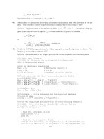
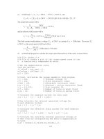
(b) A MATLAB program to calculate the torque-speed characteristic of this motor is shown below:

% M-file: prob9_17.m
% M-file to create a plot of the torque-speed curve of the
% a cumulatively compounded dc motor.

% Get the magnetization curve.
load p96_mag.dat;
if_values = p96_mag(:,1);
ea_values = p96_mag(:,2);
n_0 = 1200;

% First, initialize the values needed in this program.
v_t = 240; % Terminal voltage (V)
r_f = 200; % Field resistance (ohms)
r_adj = 120; % Adjustable resistance (ohms)
r_a = 0.19; % Armature + series resistance (ohms)
i_l = 0:2:100; % Line currents (A)
n_f = 1500; % Number of turns on shunt field
n_se = 12; % Number of turns on series field

% Calculate the armature current for each load.
i_a = i_l - v_t / (r_f + r_adj);

% Now calculate the internal generated voltage for

% each armature current.
e_a = v_t - i_a * r_a;

% Calculate the effective field current for each armature
% current.
i_f = v_t / (r_f + r_adj) + (n_se / n_f) * i_a;

% Calculate the resulting internal generated voltage at
% 1800 r/min by interpolating the motor's magnetization
% curve.
e_a0 = interp1(if_values,ea_values,i_f);

238

% Calculate the resulting speed from Equation (9-13).
n = ( e_a ./ e_a0 ) * n_0;

% Calculate the induced torque corresponding to each
% speed from Equations (8-55) and (8-56).
t_ind = e_a .* i_a ./ (n * 2 * pi / 60);

% Plot the torque-speed curves
figure(1);
plot(t_ind,n,'b-','LineWidth',2.0);
xlabel('\bf\tau_{ind} (N-m)');
ylabel('\bf\itn_{m} \rm\bf(r/min)');
title ('\bfCumulatively-Compounded DC Motor Torque-Speed
Characteristic');
axis([0 200 900 1600]);
grid on;

The resulting torque-speed characteristic is shown below:

(c) The no-load speed of this machine is the same as the no-load speed of the corresponding shunt dc
motor with
adj
R = 120
Ω
, which is 1125 r/min. The speed regulation of this motor is thus

nl fl
fl
1125 r/min - 915 r/min
SR 100% 100% 23.0%
915 r/min
nn
n
−
=×= ×=

9-18. The motor is reconnected differentially compounded with
adj
R = 120
Ω
. Derive the shape of its torque-
speed characteristic.
S
OLUTION
A MATLAB program to calculate the torque-speed characteristic of this motor is shown below:

% M-file: prob9_18.m

% M-file to create a plot of the torque-speed curve of the

239
% a differentially compounded dc motor.

% Get the magnetization curve.
load p96_mag.dat;
if_values = p96_mag(:,1);
ea_values = p96_mag(:,2);
n_0 = 1200;

% First, initialize the values needed in this program.
v_t = 240; % Terminal voltage (V)
r_f = 200; % Field resistance (ohms)
r_adj = 120; % Adjustable resistance (ohms)
r_a = 0.19; % Armature + series resistance (ohms)
i_l = 0:2:40; % Line currents (A)
n_f = 1500; % Number of turns on shunt field
n_se = 12; % Number of turns on series field

% Calculate the armature current for each load.
i_a = i_l - v_t / (r_f + r_adj);

% Now calculate the internal generated voltage for
% each armature current.
e_a = v_t - i_a * r_a;

% Calculate the effective field current for each armature
% current.
i_f = v_t / (r_f + r_adj) - (n_se / n_f) * i_a;

% Calculate the resulting internal generated voltage at
% 1800 r/min by interpolating the motor's magnetization
% curve.
e_a0 = interp1(if_values,ea_values,i_f);

% Calculate the resulting speed from Equation (9-13).
n = ( e_a ./ e_a0 ) * n_0;

% Calculate the induced torque corresponding to each
% speed from Equations (8-55) and (8-56).
t_ind = e_a .* i_a ./ (n * 2 * pi / 60);

% Plot the torque-speed curves
figure(1);
plot(t_ind,n,'b-','LineWidth',2.0);
xlabel('\bf\tau_{ind} (N-m)');
ylabel('\bf\itn_{m} \rm\bf(r/min)');
title ('\bfDifferentially-Compounded DC Motor Torque-Speed
Characteristic');
axis([0 200 900 1600]);
grid on;

240
The resulting torque-speed characteristic is shown below:

This curve is plotted on the same scale as the torque-speed curve in Problem 6-17. Compare the two
curves.
9-19. A series motor is now constructed from this machine by leaving the shunt field out entirely. Derive the
torque-speed characteristic of the resulting motor.

S
OLUTION
This motor will have extremely high speeds, since there are only a few series turns, and the flux
in the motor will be very small. A MATLAB program to calculate the torque-speed characteristic of this
motor is shown below:

% M-file: prob9_19.m
% M-file to create a plot of the torque-speed curve of the
% a series dc motor. This motor was formed by removing
% the shunt field from the cumulatively-compounded machine
% if Problem 9-17.

% Get the magnetization curve.
load p96_mag.dat;
if_values = p96_mag(:,1);
ea_values = p96_mag(:,2);
n_0 = 1200;

% First, initialize the values needed in this program.
v_t = 240; % Terminal voltage (V)
r_a = 0.19; % Armature + series resistance (ohms)
i_l = 20:1:45; % Line currents (A)
n_f = 1500; % Number of turns on shunt field
n_se = 12; % Number of turns on series field

% Calculate the armature current for each load.
i_a = i_l;

241

% Now calculate the internal generated voltage for
% each armature current.
e_a = v_t - i_a * r_a;

% Calculate the effective field current for each armature
% current. (Note that the magnetization curve is defined
% in terms of shunt field current, so we will have to
% translate the series field current into an equivalent
% shunt field current.
i_f = (n_se / n_f) * i_a;

% Calculate the resulting internal generated voltage at
% 1800 r/min by interpolating the motor's magnetization
% curve.
e_a0 = interp1(if_values,ea_values,i_f);

% Calculate the resulting speed from Equation (9-13).
n = ( e_a ./ e_a0 ) * n_0;

% Calculate the induced torque corresponding to each
% speed from Equations (8-55) and (8-56).
t_ind = e_a .* i_a ./ (n * 2 * pi / 60);

% Plot the torque-speed curves
figure(1);
plot(t_ind,n,'b-','LineWidth',2.0);
xlabel('\bf\tau_{ind} (N-m)');
ylabel('\bf\itn_{m} \rm\bf(r/min)');
title ('\bfSeries DC Motor Torque-Speed Characteristic');
grid on;

The resulting torque-speed characteristic is shown below:


242
The extreme speeds in this characteristic are due to the very light flux in the machine. To make a practical
series motor out of this machine, it would be necessary to include 20 to 30 series turns instead of 12.
9-20. An automatic starter circuit is to be designed for a shunt motor rated at 15 hp, 240 V, and 60 A. The
armature resistance of the motor is 0.15
Ω
, and the shunt field resistance is 40
Ω
. The motor is to start
with no more than 250 percent of its rated armature current, and as soon as the current falls to rated value,
a starting resistor stage is to be cut out. How many stages of starting resistance are needed, and how big
should each one be?
S
OLUTION
The rated line current of this motor is 60 A, and the rated armature current is
ALF
III=− = 60
A – 6 A = 54 A. The maximum desired starting current is (2.5)(54 A) = 135 A. Therefore, the total initial
starting resistance must be

start,1
240 V
1.778
135 A
A
RR+= = Ω

start,1
1.778 0.15 1.628 R =Ω−Ω=Ω

The current will fall to rated value when
A
E rises to

()()
240 V 1.778 54 A 144 V
A
E =−Ω =
At that time, we want to cut out enough resistance to get the current back up to 135 A. Therefore,

start,2
240 V 144 V
0.711
135 A
A
RR
−
+= =Ω

start,2
0.711 0.15 0.561 R =Ω−Ω=Ω
With this resistance in the circuit, the current will fall to rated value when
A
E rises to

(

)
(
)
240 V 0.711 54 A 201.6 V
A
E =−Ω =

At that time, we want to cut out enough resistance to get the current back up to 185 A. Therefore,

start,3
240 V 201.6 V
0.284
135 A
A
RR
−
+= = Ω


start,3
0.284 0.15 0.134 R =Ω−Ω=Ω
With this resistance in the circuit, the current will fall to rated value when
A
E
rises to

()()
240 V 0.284 54 A 224.7 V
A
E =−Ω =

If the resistance is cut out when
A
E reaches 228,6 V, the resulting current is

240 V 224.7 V
102 A 135 A
0.15
A
I
−
==<
Ω
,
so there are only three stages of starting resistance. The three stages of starting resistance can be found
from the resistance in the circuit at each state during starting.

start,1 1 2 3
1.628 RRRR=++= Ω

start,2 2 3
0.561 RRR=+= Ω


start,3 3
0.134 RR== Ω
Therefore, the starting resistances are

1
1.067 R =Ω

2
0.427 R =Ω

3
0.134 R =Ω

243
9-21. A 15-hp 120-V 1800 r/min shunt dc motor has a full-load armature current of 60 A when operating at rated
conditions. The armature resistance of the motor is
A
R = 0.15
Ω
, and the field resistance
F
R is 80
Ω
.
The adjustable resistance in the field circuit
adj
R may be varied over the range from 0 to 200
Ω
and is
currently set to 90
Ω
. Armature reaction may be ignored in this machine. The magnetization curve for this
motor, taken at a speed of 1800 r/min, is given in tabular form below:
E
A
, V

5 78 95 112 118 126
I
F
, A

0.00 0.80 1.00 1.28 1.44 2.88
Note: An electronic version of this magnetization curve can be found in file
prob9_21_mag.dat
, which can be used with MATLAB programs. Column
1 contains field current in amps, and column 2 contains the internal generated
voltage E
A
in volts.
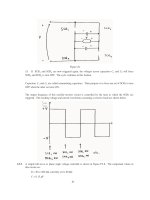
(a) What is the speed of this motor when it is running at the rated conditions specified above?
(b) The output power from the motor is 7.5 hp at rated conditions. What is the output torque of the motor?
(c) What are the copper losses and rotational losses in the motor at full load (ignore stray losses)?
(d) What is the efficiency of the motor at full load?
(e) If the motor is now unloaded with no changes in terminal voltage or
R
adj
, what is the no-load speed of
the motor?
(f) Suppose that the motor is running at the no-load conditions described in part (e). What would happen
to the motor if its field circuit were to open? Ignoring armature reaction, what would the final steady-
state speed of the motor be under those conditions?
(g) What range of no-load speeds is possible in this motor, given the range of field resistance adjustments
available with
adj
R
?

S
OLUTION

(a) If
adj
R = 90
Ω
, the total field resistance is 170
Ω
, and the resulting field current is

adj
230 V
1.35 A
90 80
T
F
F
V
I
RR
== =
+Ω+Ω

This field current would produce a voltage
Ao
E of 221 V at a speed of
o
n = 1800 r/min. The actual
A

E is

(
)
(
)
230 V 60 A 0.15 221 V
ATAA
EVIR=− = − Ω=

so the actual speed will be

()
221 V
1800 r/min 1800 r/min
221 V
A
o
Ao
E
nn
E
== =

(b) The output power is 7.5 hp and the output speed is 1800 r/min at rated conditions, therefore, the
torque is

()( )
()
out

out
15 hp 746 W/hp
59.4 N m
2 rad 1 min
1800 r/min
1 r 60 s
m
P
τ
π
ω
== = ⋅




(c) The copper losses are

244

(
)
(
)
(
)
(
)
2
2

CU
60 A 0.15 230 V 1.35 A 851 W
AA FF
PIRVI=+= Ω+ =

The power converted from electrical to mechanical form is

()()
conv
221 V 60 A 13,260 W
AA
PEI== =
The output power is

()( )
OUT
15 hp 746 W/hp 11,190 WP ==
Therefore, the rotational losses are

rot conv OUT
13,260 W 11,190 W 2070 WPP P=−= − =

(d) The input power to this motor is

()
()( )
IN
230 V 60 A 1.35 A 14,100 W
TA F
PVII=+= + =

Therefore, the efficiency is

OUT
IN
11,190 W
100% 100% 79.4%
14,100 W
P
P
η
=× = × =
(e) The no-load
A
E will be 230 V, so the no-load speed will be

()
230 V
1800 r/min 1873 r/min
221 V
A
o
Ao
E
nn
E
== =

(f) If the field circuit opens, the field current would go to zero
⇒
φ

drops to
res
φ
⇒
A
E
↓ ⇒
A
I
↑⇒
ind
τ
↑

⇒
n
↑
to a very high speed. If
F
I = 0 A,
Ao
E = 8.5 V at 1800 r/min, so

()
230 V
1800 r/min 48,700 r/min
8.5 V
A
o
Ao

E
nn
E
== =

(In reality, the motor speed would be limited by rotational losses, or else the motor will destroy itself first.)
(g) The maximum value of
adj
R
= 200 Ω, so

adj
230 V
0.821 A
200 80
T
F
F
V
I
RR
== =
+Ω+Ω

This field current would produce a voltage
Ao
E
of 153 V at a speed of
o
n

= 1800 r/min. The actual
A
E is
230 V, so the actual speed will be

()
230 V
1800 r/min 2706 r/min
153 V
A
o
Ao
E
nn
E
== =

The minimum value of
adj
R = 0
Ω
, so

adj
230 V
2.875 A
0 80
T
F
F

V
I
RR
== =
+Ω+Ω

This field current would produce a voltage
Ao
E of about 242 V at a speed of
o
n = 1800 r/min. The actual
A
E
is 230 V, so the actual speed will be

245

()
230 V
1800 r/min 1711 r/min
242 V
A
o
Ao
E
nn
E
== =

9-22. The magnetization curve for a separately excited dc generator is shown in Figure P9-7. The generator is

rated at 6 kW, 120 V, 50 A, and 1800 r/min and is shown in Figure P9-8. Its field circuit is rated at 5A.
The following data are known about the machine:

Note: An electronic version of this magnetization curve can be found in file
p97_mag.dat
, which can be used with MATLAB programs. Column 1
contains field current in amps, and column 2 contains the internal generated
voltage E
A
in volts.

246

0.18
A
R =Ω 120 V
F
V =

adj
0 to 30 R =Ω 24
F
R =Ω
1000 turns per pole
F
N =
Answer the following questions about this generator, assuming no armature reaction.
(a) If this generator is operating at no load, what is the range of voltage adjustments that can be achieved
by changing
R

adj
?

(b) If the field rheostat is allowed to vary from 0 to 30
Ω
and the generator’s speed is allowed to vary from
1500 to 2000 r/min, what are the maximum and minimum no-load voltages in the generator?
S
OLUTION

(a) If the generator is operating with no load at 1800 r/min, then the terminal voltage will equal the
internal generated voltage
A
E . The maximum possible field current occurs when
adj
R = 0
Ω
. The current
is

,max
adj
120 V
5 A
24 0
F
F
F
V
I

RR
== =
+Ω+Ω

From the magnetization curve, the voltage
Ao
E at 1800 r/min is 129 V. Since the actual speed is 1800
r/min, the maximum no-load voltage is 129 V.
The minimum possible field current occurs when
adj
R = 30
Ω
. The current is

,max
adj
120 V
2.22 A
24 30
F
F
F
V
I
RR
== =
+Ω+Ω

From the magnetization curve, the voltage
Ao

E at 1800 r/min is 87.4 V. Since the actual speed is 1800
r/min, the minimum no-load voltage is 87 V.
(b) The maximum voltage will occur at the highest current and speed, and the minimum voltage will
occur at the lowest current and speed. The maximum possible field current occurs when
adj
R = 0
Ω
. The
current is

,max
adj
120 V
5 A
24 0
F
F
F
V
I
RR
== =
+Ω+Ω

From the magnetization curve, the voltage
Ao
E at 1800 r/min is 129 V. Since the actual speed is 2000
r/min, the maximum no-load voltage is

247

A
Ao o
En
En
=


()
2000 r/min
129 V 143 V
1800 r/min
AAo
o
n
EE
n
== =

The minimum possible field current occurs when
adj
R = 30
Ω
. The current is

,max
adj
120 V
2.22 A
24 30

F
F
F
V
I
RR
== =
+Ω+Ω

From the magnetization curve, the voltage
Ao
E
at 1800 r/min is 87.4 V. Since the actual speed is 1500
r/min, the maximum no-load voltage is

A
Ao o
En
En
=


()
1500 r/min
87.4 V 72.8 V
1800 r/min
AAo
o
n
EE

n
== =

9-23. If the armature current of the generator in Problem 9-22 is 50 A, the speed of the generator is 1700 r/min,
and the terminal voltage is 106 V, how much field current must be flowing in the generator?
S
OLUTION
The internal generated voltage of this generator is

(
)
(
)
106 V 50 A 0.18 115 V
ATAA
EVIR=+ = + Ω=

at a speed of 1700 r/min. This corresponds to an
Ao
E at 1800 r/min of

A
Ao o
En
En
=


()
1800 r/min

115 V 121.8 V
1700 r/min
o
Ao A
n
EE
n
== =

From the magnetization curve, this value of
Ao
E
requires a field current of 4.2 A.
9-24. Assuming that the generator in Problem 9-22 has an armature reaction at full load equivalent to 400
A
⋅turns of magnetomotive force, what will the terminal voltage of the generator be when
F
I
= 5 A,
m
n
=
1700 r/min, and
A
I
= 50 A?
S
OLUTION
When
F

I is 5 A and the armature current is 50 A, the magnetomotive force in the generator is

(
)
(
)
net AR
1000 turns 5 A 400 A turns 4600 A turns
F
NI=−= − ⋅ = ⋅FF

or
*
net
/
4600 A turns / 1000 turns 4.6 A
FF
IN==⋅ =F

The equivalent internal generated voltage
Ao
E of the generator at 1800 r/min would be 126 V. The actual
voltage at 1700 r/min would be

()
1700 r/min
126 V 119 V
1800 r/min
AAo
o

n
EE
n
== =

Therefore, the terminal voltage would be

(
)
(
)
119 V 50 A 0.18 110 V
TAAA
VEIR=− = − Ω=


248
9-25. The machine in Problem 9-22 is reconnected as a shunt generator and is shown in Figure P9-9. The shunt
field resistor
R
adj
is adjusted to 10
Ω
, and the generator’s speed is 1800 r/min.

(a) What is the no-load terminal voltage of the generator?
(b) Assuming no armature reaction, what is the terminal voltage of the generator with an armature current
of 20 A? 40 A?
(c) Assuming an armature reaction equal to 200 A
⋅

turns at full load, what is the terminal voltage of the
generator with an armature current of 20 A? 40 A?
(d) Calculate and plot the terminal characteristics of this generator with and without armature reaction.
S
OLUTION

(a) The total field resistance of this generator is 34
Ω, and the no-load terminal voltage can be found
from the intersection of the resistance line with the magnetization curve for this generator. The
magnetization curve and the field resistance line are plotted below. As you can see, they intersect at a
terminal voltage of 112 V.


249
(b) At an armature current of 20 A, the internal voltage drop in the armature resistance is
()( )
V 6.3 0.18 A 20 =Ω . As shown in the figure below, there is a difference of 3.6 V between
A
E and
T
V
at a terminal voltage of about 106 V.

A MATLAB program to locate the position where the triangle exactly fits between the
A
E
and
T
V
lines is

shown below. This program created the plot shown above. Note that there are actually two places where
the difference between the
A
E and
T
V lines is 3.6 volts, but the low-voltage one of them is unstable. The
code shown in bold face below prevents the program from reporting that first (unstable) point.

% M-file: prob9_25b.m
% M-file to create a plot of the magnetization curve and the
% field current curve of a shunt dc generator, determining
% the point where the difference between them is 3.6 V.

% Get the magnetization curve. This file contains the
% three variables if_values, ea_values, and n_0.
clear all
load p97_mag.dat;
if_values = p97_mag(:,1);
ea_values = p97_mag(:,2);
n_0 = 1800;

% First, initialize the values needed in this program.
r_f = 24; % Field resistance (ohms)
r_adj = 10; % Adjustable resistance (ohms)
r_a = 0.19; % Armature + series resistance (ohms)
i_f = 0:0.02:6; % Field current (A)
n = 1800; % Generator speed (r/min)

% Calculate Ea versus If
Ea = interp1(if_values,ea_values,i_f);

250
% Calculate Vt versus If
Vt = (r_f + r_adj) * i_f;

% Find the point where the difference between the two
% lines is 3.6 V. This will be the point where the line
% line "Ea - Vt - 3.6" goes negative. That will be a
% close enough estimate of Vt.
diff = Ea - Vt - 3.6;

% This code prevents us from reporting the first (unstable)
% location satisfying the criterion.
was_pos = 0;
for ii = 1:length(i_f);
if diff(ii) > 0
was_pos = 1;
end
if ( diff(ii) < 0 & was_pos == 1 )
break;
end;
end;

% We have the intersection. Tell user.
disp (['Ea = ' num2str(Ea(ii)) ' V']);
disp (['Vt = ' num2str(Vt(ii)) ' V']);
disp (['If = ' num2str(i_f(ii)) ' A']);

% Plot the curves

figure(1);
plot(i_f,Ea,'b-','LineWidth',2.0);
hold on;
plot(i_f,Vt,'k ','LineWidth',2.0);
% Plot intersections
plot([i_f(ii) i_f(ii)], [0 Ea(ii)], 'k-');
plot([0 i_f(ii)], [Vt(ii) Vt(ii)],'k-');
plot([0 i_f(ii)], [Ea(ii) Ea(ii)],'k-');
xlabel('\bf\itI_{F} \rm\bf(A)');
ylabel('\bf\itE_{A} \rm\bf or \itV_{T}');
title ('\bfPlot of \itE_{A} \rm\bf and \itV_{T} \rm\bf vs field
current');
axis ([0 5 0 150]);
set(gca,'YTick',[0 10 20 30 40 50 60 70 80 90 100 110 120 130 140
150]')
set(gca,'XTick',[0 0.5 1.0 1.5 2.0 2.5 3.0 3.5 4.0 4.5 5.0]')
legend ('Ea line','Vt line',4);
hold off;
grid on;
At an armature current of 40 A, the internal voltage drop in the armature resistance is
()( )
V 2.7 0.18 A 40 =Ω . As shown in the figure below, there is a difference of 7.2 V between
A
E and
T
V at a terminal voltage of about 98 V.

251

(c) The rated current of this generated is 50 A, so 20 A is 40% of full load. If the full load armature

reaction is 200 A
⋅turns, and if the armature reaction is assumed to change linearly with armature current,
then the armature reaction will be 80 A
⋅
turns. The figure below shows that a triangle consisting of 3.6 V
and (80 A
⋅turns)/(1000 turns) = 0.08 A fits exactly between the
A
E
and
T
V
lines at a terminal voltage of
103 V.

252

The rated current of this generated is 50 A, so 40 A is 80% of full load. If the full load armature reaction
is 200 A
⋅turns, and if the armature reaction is assumed to change linearly with armature current, then the
armature reaction will be 160 A
⋅
turns. There is no point where a triangle consisting of 3.6 V and (80
A
⋅
turns)/(1000 turns) = 0.16 A fits exactly between the
A
E
and
T

V
lines, so this is not a stable operating
condition.
(c) A MATLAB program to calculate the terminal characteristic of this generator without armature
reaction is shown below:

% M-file: prob9_25d.m
% M-file to calculate the terminal characteristic of a shunt
% dc generator without armature reaction.

% Get the magnetization curve. This file contains the
% three variables if_values, ea_values, and n_0.
load p97_mag.dat;
if_values = p97_mag(:,1);
ea_values = p97_mag(:,2);
n_0 = 1800;

% First, initialize the values needed in this program.
r_f = 24; % Field resistance (ohms)
r_adj = 10; % Adjustable resistance (ohms)
r_a = 0.18; % Armature + series resistance (ohms)
i_f = 0:0.005:6; % Field current (A)
n = 1800; % Generator speed (r/min)

253

% Calculate Ea versus If
Ea = interp1(if_values,ea_values,i_f);

% Calculate Vt versus If

Vt = (r_f + r_adj) * i_f;

% Find the point where the difference between the two
% lines is exactly equal to i_a*r_a. This will be the
% point where the line line "Ea - Vt - i_a*r_a" goes
% negative.
i_a = 0:1:50;
for jj = 1:length(i_a)

% Get the voltage difference
diff = Ea - Vt - i_a(jj)*r_a;

% This code prevents us from reporting the first (unstable)
% location satisfying the criterion.
was_pos = 0;
for ii = 1:length(i_f);
if diff(ii) > 0
was_pos = 1;
end
if ( diff(ii) < 0 & was_pos == 1 )
break;
end;
end;

% Save terminal voltage at this point
v_t(jj) = Vt(ii);
i_l(jj) = i_a(jj) - v_t(jj) / ( r_f + r_adj);

end;

% Plot the terminal characteristic
figure(1);
plot(i_l,v_t,'b-','LineWidth',2.0);
xlabel('\bf\itI_{L} \rm\bf(A)');
ylabel('\bf\itV_{T} \rm\bf(V)');
title ('\bfTerminal Characteristic of a Shunt DC Generator');
hold off;
axis( [ 0 50 0 120]);
grid on;

254
The resulting terminal characteristic is shown below:

A MATLAB program to calculate the terminal characteristic of this generator with armature reaction is
shown below:

% M-file: prob9_25d2.m
% M-file to calculate the terminal characteristic of a shunt
% dc generator with armature reaction.

% Get the magnetization curve. This file contains the
% three variables if_values, ea_values, and n_0.
clear all
load p97_mag.dat;
if_values = p97_mag(:,1);
ea_values = p97_mag(:,2);
n_0 = 1800;

% First, initialize the values needed in this program.
r_f = 24; % Field resistance (ohms)

r_adj = 10; % Adjustable resistance (ohms)
r_a = 0.18; % Armature + series resistance (ohms)
i_f = 0:0.005:6; % Field current (A)
n = 1800; % Generator speed (r/min)
n_f = 1000; % Number of field turns

% Calculate Ea versus If
Ea = interp1(if_values,ea_values,i_f);

% Calculate Vt versus If
Vt = (r_f + r_adj) * i_f;

% Find the point where the difference between the Ea
% armature reaction line and the Vt line is exactly
% equal to i_a*r_a. This will be the point where

255
% the line "Ea_ar - Vt - i_a*r_a" goes negative.
i_a = 0:1:37;
for jj = 1:length(i_a)

% Calculate the equivalent field current due to armature
% reaction.
i_ar = (i_a(jj) / 50) * 200 / n_f;

% Calculate the Ea values modified by armature reaction
Ea_ar = interp1(if_values,ea_values,i_f - i_ar);

% Get the voltage difference
diff = Ea_ar - Vt - i_a(jj)*r_a;

% This code prevents us from reporting the first (unstable)
% location satisfying the criterion.
was_pos = 0;
for ii = 1:length(i_f);
if diff(ii) > 0
was_pos = 1;
end
if ( diff(ii) < 0 & was_pos == 1 )
break;
end;
end;

% Save terminal voltage at this point
v_t(jj) = Vt(ii);
i_l(jj) = i_a(jj) - v_t(jj) / ( r_f + r_adj);

end;

% Plot the terminal characteristic
figure(1);
plot(i_l,v_t,'b-','LineWidth',2.0);
xlabel('\bf\itI_{L} \rm\bf(A)');
ylabel('\bf\itV_{T} \rm\bf(V)');
title ('\bfTerminal Characteristic of a Shunt DC Generator w/AR');
hold off;
axis([ 0 50 0 120]);
grid on;

256

The resulting terminal characteristic is shown below:

9-26. If the machine in Problem 9-25 is running at 1800 r/min with a field resistance R
adj
= 10
Ω
and an
armature current of 25 A, what will the resulting terminal voltage be? If the field resistor decreases to 5
Ω

while the armature current remains 25 A, what will the new terminal voltage be? (Assume no armature
reaction.)
S
OLUTION
If
A
I = 25 A, then
(
)
(
)
25 A 0.18
AA
IR =Ω
= 4.5 V. The point where the distance between the
A
E and
T
V curves is exactly 4.5 V corresponds to a terminal voltage of 104 V, as shown below.

257
If
R
adj
decreases to 5
Ω
, the total field resistance becomes 29
Ω
, and the terminal voltage line gets
shallower. The new point where the distance between the
A
E
and
T
V
curves is exactly 4.5 V corresponds
to a terminal voltage of 115 V, as shown below.

Note that decreasing the field resistance of the shunt generator increases the terminal voltage.
9-27. A 120-V 50-A cumulatively compounded dc generator has the following characteristics:

0.21
AS
RR+= Ω

1000 turns
F
N =

20
F
R =Ω

SE
20 turnsN =


adj
0 to 30 , set to 10 R =Ω Ω

1800 r/min
m
n =

The machine has the magnetization curve shown in Figure P9-7. Its equivalent circuit is shown in Figure
P9-10. Answer the following questions about this machine, assuming no armature reaction.

(a) If the generator is operating at no load, what is its terminal voltage?
(b) If the generator has an armature current of 20 A, what is its terminal voltage?

258
(c) If the generator has an armature current of 40 A, what is its terminal voltage'?
(d) Calculate and plot the terminal characteristic of this machine.
S
OLUTION

(a) The total field resistance of this generator is 30
Ω

, and the no-load terminal voltage can be found
from the intersection of the resistance line with the magnetization curve for this generator. The
magnetization curve and the field resistance line are plotted below. As you can see, they intersect at a
terminal voltage of 121 V.

(b) If the armature current is 20 A, then the effective field current contribution from the armature current

()
SE
20
20 A 0.4 A
1000
A
F
N
I
N
==

and the
()
AA S
IR R+
voltage drop is
()
(
)
(
)
20 A 0.21 4.2 V

AA S
IR R+= Ω=
. The location where the
triangle formed by
SE
A
F
N
I
N
and
AA
IR
exactly fits between the
A
E
and
T
V
lines corresponds to a terminal
voltage of 120 V, as shown below.